Measurement of ${\boldmath\eta\eta}$ production in two-photon collisions

Abstract

We report the first measurement of the differential cross section for the process $\gamma\gamma\to\eta\eta$ in the kinematic range above the $\eta\eta$ threshold, $1.096~{}{\rm GeV}<W<3.8~{}{\rm GeV}$ over nearly the entire solid angle range, $|\cos\theta^{*}|\leq 0.9$ or $\leq 1.0$ depending on $W$, where $W$ and $\theta^{*}$ are the energy and $\eta$ scattering angle, respectively, in the $\gamma\gamma$ center-of-mass system. The results are based on a 393 fb^-1 data sample collected with the Belle detector at the KEKB $e^{+}e^{-}$ collider. In the $W$ range 1.1–2.0 GeV/$c^{2}$ we perform an analysis of resonance amplitudes for various partial waves, and at higher energy we compare the energy and the angular dependences of the cross section with predictions of theoretical models and extract contributions of the $\chi_{cJ}$ charmonia.

The Belle Collaboration

I Introduction

Measurements of exclusive hadronic final states in two-photon collisions provide valuable information concerning the physics of light and heavy-quark resonances, perturbative and non-perturbative QCD and hadron-production mechanisms. So far, we, the Belle Collaboration, have measured the production cross sections for charged-pion pairs mori1 ; mori2 ; nkzw , charged and neutral-kaon pairs nkzw ; kabe ; wtchen , and proton-antiproton pairs kuo . We have also analyzed $D$-meson-pair production and observe a new charmonium state identified as the $\chi_{c2}(2P)$ uehara . Recently, we have examined $\omega J/\psi$ and $\phi J/\psi$ production and also found charmonium-like structures in these final states uehara2 ; shen .

In addition, we have measured the production cross section for the $\pi^{0}\pi^{0}$ and $\eta\pi^{0}$ final states pi0pi0 ; pi0pi02 ; etapi0 . The statistics of these measurements are two to three orders of magnitude higher than in pre-B-factory measurements past_exp , opening a new era in studies of two-photon physics.

In the present study, we report measurements of the differential cross sections, $d\sigma/d|\cos\theta^{*}|$, for the process $\gamma\gamma\to\eta\eta$ in a wide two-photon center-of-mass (c.m.) energy ($W$) range from the $\eta\eta$ mass threshold 1.096 GeV to 3.8 GeV, and in the c.m. angular range, $|\cos\theta^{*}|\leq 1$ ($0.9$) for $W\leq 2.0~{}{\rm GeV}$ ($W>2.0~{}{\rm GeV}$). In this analysis, we use the $\eta\to\gamma\gamma$ decay mode only because the $\eta\to\pi^{+}\pi^{-}\pi^{0}$ decay mode has a much smaller product of efficiency and branching fraction.

The $I^{G}J^{PC}$ quantum numbers of a meson produced by two photons and decaying into $\eta\eta$ are restricted to be $0^{+}$(even)⁺⁺, that is, those of $f_{J={\rm even}}$ or $\chi_{cJ={\rm even}}$ mesons. A long-standing puzzle in QCD is the existence and structure of low mass scalar mesons. In the $I=0$ sector, we recently observed a peaking structure at the $f_{0}(980)$ mass in both the $\gamma\gamma\to\pi^{+}\pi^{-}$ and $\gamma\gamma\to\pi^{0}\pi^{0}$ channels mori1 ; pi0pi0 . Our analysis also suggests the existence of another $f_{0}$ meson in the 1.2–1.5 GeV region that couples to two photons pi0pi0 . The significant $s\bar{s}$ component in the $\eta$ meson implies a connection of this reaction to the $K^{+}K^{-}$ kabe and $K^{0}\bar{K}^{0}$ wtchen processes.

At higher energies ($W>2.4$ GeV), we can invoke a quark model. In leading-order calculations, the ratio of the $\eta\pi^{0}$ or $\eta\eta$ cross section to that of $\pi^{0}\pi^{0}$ is predicted. Analyses of energy and angular distributions of these cross sections are essential to determine properties of the observed resonances and to test the validity of QCD based models bl ; handbag ; handbag2 involving $q\bar{q}$ production and SU(3) flavor symmetry. It is also interesting to compare the behavior of $\eta\eta$ production with that of $K^{+}K^{-}$ and $K^{0}_{S}K^{0}_{S}$, which have been measured by the Belle experiment nkzw ; wtchen . The cross section for the $\gamma\gamma\to\eta\eta$ process has not been measured so far.

The organization of this paper is as follows. In Sec. II, the experimental apparatus and event selection are described. Signal yields and backgrounds are discussed in Sec. III. Differential cross sections are then extracted in Sec. IV. In Sec. V the $f_{2}(1270)$, $f_{2}^{\prime}(1525)$ and other possible resonances are studied by parameterizing partial wave amplitudes. The behavior of differential cross sections and $W$ dependence of the integrated cross sections at higher energy region ($W>2.4~{}{\rm GeV}$) are compared to QCD predictions in Sec. VI. Finally in Sec. VII, a summary and conclusion are given.

II Experimental apparatus and event selection

Events with all neutral final states are extracted from the data collected by the Belle experiment. In this section, the Belle detector and event selection procedure are described.

II.1 Experimental apparatus

A comprehensive description of the Belle detector is given elsewhere belle . We mention here only those detector components that are essential for the present measurement. Charged tracks are reconstructed from hit information in the silicon vertex detector and the central drift chamber (CDC) located in a uniform 1.5 T solenoidal magnetic field. The detector solenoid is oriented along the $z$ axis, which points in the direction opposite to that of the positron beam. Photon detection and energy measurements are performed with a CsI(Tl) electromagnetic calorimeter (ECL).

For this all-neutral final state, we require that there be no reconstructed tracks coming from the vicinity of the nominal collision point. Therefore, the CDC is used to veto events with charged track(s). The photons from a decay of the $\eta$ meson are detected and their momentum vectors are measured by the ECL. The ECL is also used to trigger signal events. Two kinds of ECL triggers are used to select events of interest: the total ECL energy deposit in the acceptance region used by the trigger (see the next subsection) is greater than 1.15 GeV (the “HiE” trigger), or four or more ECL clusters above an energy threshold of 110 MeV in segments of the ECL (the “Clst4” trigger). The above energy thresholds are determined by studying the correlations between the two triggers in the experimental data.

II.2 Experimental data and data filtering

We use a 393 fb^-1 data sample accumulated by the Belle detector at the KEKB asymmetric-energy $e^{+}e^{-}$ collider kekb . For an early part of Belle data taking, all neutral final states were not recorded. Thus, this data set is smaller than the hadronic data sample available at Belle.

The data were recorded at several $e^{+}e^{-}$ c.m. energy regions summarized in Table 1. We combine the results from the different beam energies, because the $e^{+}e^{-}$ c.m. energy is more than twice our $\gamma\gamma$ c.m. energy range for any of the beam energies, and the beam-energy dependence of the two-photon luminosity function is rather small. We generate most of the signal Monte-Carlo (MC) events and calculate the two-photon luminosity function for 10.58 GeV. We then derive a correction factor for the other beam energies. The correction is less than 0.5% over the full range of $\gamma\gamma$ cm energies considered here. The signal MC and the beam energy dependences are described in Sec. IV.C.

The analysis is carried out in the “zero-tag” mode, where neither the recoil electron nor positron are detected. We restrict the virtuality of the incident photons to be small by imposing a strict requirement on the transverse-momentum balance with respect to the beam axis for the final-state hadronic system.

The filtering procedure (“Neutral Skim”) used for this analysis is the same as the one used for $\pi^{0}\pi^{0}$ and $\eta\pi^{0}$ studies pi0pi0 ; pi0pi02 ; etapi0 . The important requirements in this filter are the following: there are no tracks originating in the beam collision region and having a transverse momentum greater than 0.1 GeV/$c$ in the laboratory frame; two or more photons that satisfy a specified energy or transverse-momentum criterion; this requirement is satisfied when there are three or more photons each with an energy above 100 MeV. The performance of the ECL triggers is studied in detail using $\pi^{0}\pi^{0}$ events pi0pi0 . We also study the trigger thresholds using the $\eta\eta$ signal samples.

Table 1: Data sample: integrated luminosities and energies

$e^{+}e^{-}$ c.m. energy	Integrated luminosity	Runs
(GeV)	(fb-1)
10.58	286	$\Upsilon(4S)$
10.52	33	continuum
9.43 - 9.46	7.3	near $\Upsilon(1S)$
9.99 - 10.03	6.7	near $\Upsilon(2S)$
10.32 - 10.36	3.2	near $\Upsilon(3S)$
10.83 - 11.02	58	near $\Upsilon(5S)$
Total	393

II.3 Event selection

From the Neutral Skim event sample, we select $\gamma\gamma\to\eta\eta$ candidates that satisfy the following conditions:

• the total energy deposit in ECL is less than 5.7 GeV;

• each photon candidate is required to have an energy of at least 100 MeV, and events with four such photons are selected;

• the event is triggered by either the ECL trigger HiE or Clst4;

• either the sum of the energies of the photons in the acceptance region used by the trigger is larger than 1.25 GeV, or all four selected photons are within this region, where the trigger acceptance is the polar-angle range, $-0.6255<\cos\theta<+0.9563$, in the laboratory frame;

• of the three possible combinations that can be constructed from the four photons, there is one in which each invariant mass of the two photon pairs satisfies 0.52 GeV/$c^{2}<M_{\gamma\gamma\ i}<$ 0.57 GeV/$c^{2}$, where $i=1$, 2 is an index of the two-photon pairs;

• there is no neutral pion combination that is constructed from any two of the four photons with a $\chi^{2}$ smaller than 9 in the mass-constrained fit;

• the transverse momentum for the $\eta\eta$ system $|\Sigma{\mbox{{\boldmath$p$}}}_{t}^{*}|$ is required to be less than $0.05~{}{\rm GeV}/c$.

A small fraction of events contain multiple combinations of the four photons that satisfy criterion (5). In those events, we take only one combination whose residual for the nominal $\eta$ mass ($m_{\eta}=0.5478$ GeV/$c^{2}$), $(M_{\gamma\gamma 1}-m_{\eta})^{2}+(M_{\gamma\gamma 2}-m_{\eta})^{2}$, is the smallest.

We then scale the energy of the two photons with a factor that is the ratio of the nominal $\eta$ mass to the reconstructed mass, $m_{\eta}/M_{\gamma\gamma\ i}$. This is equivalent to an approximate 1C (one constraint) mass constraint fit in which the relative energy resolution ($\Delta E/E$) is independent of $E$ and the resolution in the angle measurement is much better than that of the energy. This is a good approximation for the $\eta$’s in this momentum range. Using the corrected four-momenta of the $\eta$ mesons, we calculate the invariant mass ($W$) and the transverse momentum ($|\Sigma{\mbox{{\boldmath$p$}}}_{t}^{*}|$) in the $e^{+}e^{-}$ c.m. frame for the $\eta\eta$ system and apply cut (7) above. We select 31655 candidates in the region $W<4.0$ GeV.

We define the c.m. scattering angle, $\theta^{*}$, as the scattering angle of the $\eta$. The $e^{+}e^{-}$ direction is used to approximate the axis for the polar angle calculation because the exact $\gamma\gamma$ axis is unknown for untagged events. The two-dimensional ($W$, $|\cos\theta^{*}|$) distribution of selected events is shown in Fig. 1.

The probability for a signal $\eta\eta$ event to have multiple combinations is sizable only near the threshold (about 6% at $W\sim 1.11$ GeV), but it is small (less than 2%) above $W>1.12$ GeV, according to the signal MC samples. For different choices of $\gamma$-pair combinations in an event, the $W$ values are nearly the same, but $|\cos\theta^{*}|$ can be different. As the angular distribution is observed to be flat near the threshold, which is also theoretically expected, the effect of an incorrect choice is negligibly small.

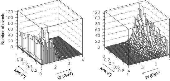
Figure 1: Two-dimensional $W$ and $|\cos\theta^{*}|$ distribution for the $\eta\eta$ candidates in data. The same distribution is viewed from two different directions. The backgrounds are not subtracted.

III Yields of the signal and backgrounds

In this section, backgrounds are identified and subtracted and the extraction of the signal yield is discussed.

III.1 Determination of non-$\eta\eta$ background

There are two kinds of background processes for the $\gamma\gamma\to\eta\eta$ signal process: non-$\eta\eta$ and $\eta\eta X$ backgrounds. The non-$\eta\eta$ background does not contain an $\eta$ pair in the final state, while the $\eta\eta X$ background includes extra particle(s) in the final state in addition to the $\eta\eta$ combination. In this measurement, the non-$\eta\eta$ contribution, arising from beam backgrounds or other physics processes, is the dominant background in the final sample.

We first determine the number of the non-$\eta\eta$ background events using the yields of $\eta\eta$ mass sidebands. After subtracting this background contribution, we check the $p_{t}$-balance distribution for the remaining component; the signal component peaks near $|\Sigma{\mbox{{\boldmath$p$}}}_{t}^{*}|=0$, while we expect that the $\eta\eta X$ background does not.

III.1.1 Defining the $\eta\eta$-mass sidebands

The $\eta\eta$-mass sidebands are defined by displacing the central points of the mass intervals in selection criterion (5) by $\pm 0.07$ GeV/$c^{2}$. Two kinds of sidebands are defined: Sideband A and Sideband B. In Sideband A, the central points for the two-dimensional mass cut for ($M_{\gamma\gamma 1}$, $M_{\gamma\gamma 2}$) are (here, we assume $M_{\gamma\gamma 1}<M_{\gamma\gamma 2}$) (0.545, 0.615) and (0.475, 0.545) in units of GeV/$c^{2}$ and the width of the range is $\pm 0.025$ GeV/$c^{2}$. Sideband B has central points (0.475, 0.475), (0.475, 0.615) and (0.615, 0.615). When there are two or more choices of $\gamma$-pair combinations in an event that fall in the same sideband box, we take the one that is closest to the nominal central point of each sideband box, ($m_{\eta}-0.07$, $m_{\eta}$) or ($m_{\eta}$, $m_{\eta}+0.07$) for Sideband A, and ($m_{\eta}+/-0.07$, $m_{\eta}+/-0.07$) for Sideband B. This is similar to the multiple candidate selection applied for the signal candidates. The $M_{\gamma\gamma}$ distributions near the signal and sideband regions are shown in Fig. 2.

We also calculate $W$ and $|\cos\theta^{*}|$ for the Sideband A and B candidates by scaling $M_{\gamma\gamma\ i}$ to $m_{\eta}$ (not to $m_{\eta}+/-0.07$, which would change the threshold mass).

III.1.2 Sideband subtraction

We subtract the sideband yield to obtain the signal component with the following formula:

$$Y=Y_{s}-0.5Y_{bA}+0.25Y_{bB},$$

where $Y$ is the signal yield after sideband subtraction, $Y_{s}$ is the yield in the observed events in the signal region, and $Y_{bA}$ ( $Y_{bB}$ ) the yield of the Sideband A (B) region. Here we model the non-$\eta$ backgrounds with a linear distribution in $M_{\gamma\gamma}$, for backgrounds with both $\eta$ non-$\eta$ and non-$\eta$ non-$\eta$ combinations. The possibility of a non-linear background component is included in the systematic error (see Sec. IV.E). The yield in the signal and sideband regions (before the sideband subtraction) is shown in Fig. 3. To obtain the differential cross sections, we subtract bin-by-bin in each two-dimensional bin of $(W,|\cos\theta^{*}|)$ with bin widths $\Delta W=20~{}{\rm MeV}$ and $\Delta|\cos\theta^{*}|=0.1$. Two or five $W$ bins are combined later in the determination of the final cross sections. Signal leakage into the sideband regions, which amounts to 2–5% of the signal size $Y$ and is larger at small $W$, is expected according to signal MC simulations. This effect is corrected in the derivation of the differential cross sections by reducing the efficiency.

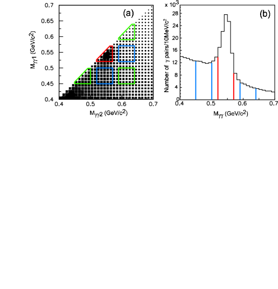
Figure 2: (a) Two-dimensional $M_{\gamma\gamma 1}$ vs. $M_{\gamma\gamma 2}$ distribution of the four-photon candidates in data. We take $M_{\gamma\gamma 1}<M_{\gamma\gamma 2}$. The $p_{t}$-balance cut with $p_{t}<0.1~{}$GeV/$c$ is applied using the photon momenta before the $m_{\eta}$ mass correction, which reduces backgrounds. Red, blue and green boxes show the signal, Sideband A and Sideband B regions, respectively. (b) A one-dimensional projection of the same distribution where the $\gamma\gamma$ pair on the opposite side is required to be in the signal mass region, 0.52–0.57 GeV/$c^{2}$. The vertical red and blue lines show the signal and two Sideband A regions, respectively. Note that there are two entries per event in the signal region.

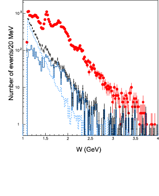
Figure 3: $W$ distributions of the yields in the signal region (closed circles with error bars, $Y_{s}$), and estimates of backgrounds of the $\eta$ non-$\eta$ component (solid histogram, $0.5(Y_{bA}-Y_{bB})$) and the non-$\eta$ non-$\eta$ component (dashed histogram, $0.25Y_{bB}$). Points with error bars show the estimated total background, $0.5Y_{bA}-0.25Y_{bB}$.

III.2 $p_{t}$-unbalanced component

We expect that the background remaining after the $\eta\eta$ sideband subtraction is very small. To confirm this, we examine the $W$ dependence of the yield ratio of the $p_{t}$-unbalanced component $R$ defined as:

$$R=\frac{Y(0.15~{}{\rm GeV}/c<|\sum\mbox{{\boldmath$p$}}_{t}^{*}|<0.20~{}{\rm GeV}/c)}{Y(|\sum\mbox{{\boldmath$p$}}_{t}^{*}|<0.05~{}{\rm GeV}/c)}\;,$$ (1)

where $Y$ is the yield after the sideband subtraction in the specified $p_{t}$ region. $R$ is plotted as a function of $W$ in Fig. 4, where any excess over the signal MC would indicate a contribution from $\eta\eta X$ background. There is such a small excess just above mass threshold. We include the effect from this possible background source into the correction and the systematic error. Non-$\eta\eta$ background is much larger near the $W$ threshold, and this excess may be due to an imperfect sideband subtraction. We apply a $-3\%$ correction for the background from this source for $W<1.2$ GeV. In the $W$ region between 1.2 GeV and 3.3 GeV, the $R$ value is consistent with the signal MC simulation. The reason why the experimental data seems to be slightly below the MC for $R$ in the 1.4 – 2.0 GeV range is not known, but the difference translated to the background ratio is negligibly small, less than 1%. For $W>3.3$ GeV, there could be much larger $\eta\eta X$ backgrounds. As described in Sec. IV.C, we do not report cross section results for $W>3.3$ GeV, and apply a $-3\%$ correction for 3.2 GeV$<W<3.3$ GeV.

We conclude that this kind of background is less than 2% throughout the $W$ region, 1.2 – 3.2 GeV, and assign 2% as the systematic error for this source for the entire $W$ region, 1.096 – 3.3 GeV. These factors are obtained by assuming a quasi-linear $|\sum\mbox{{\boldmath$p$}}_{t}^{*}|$ dependence of the background and extracting its leakage into the signal region ($|\sum\mbox{{\boldmath$p$}}_{t}^{*}|<0.05~{}{\rm GeV}/c$), which is approximately 1/6 of the yield in the $0.15~{}{\rm GeV}/c<|\sum\mbox{{\boldmath$p$}}_{t}^{*}|<0.20~{}{\rm GeV}/c$ region.

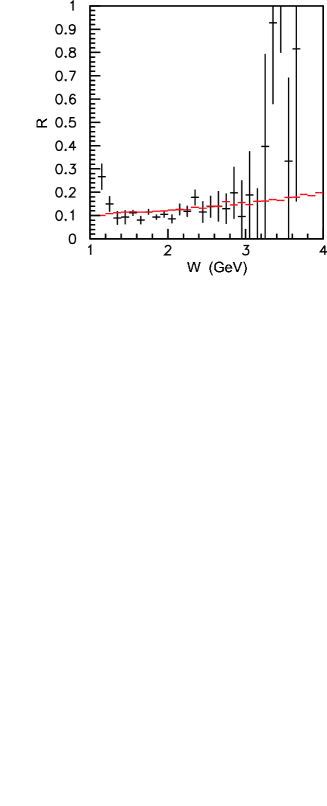
Figure 4: Energy dependence of $R$ defined in Eq.(1). It indicates the level of $\eta\eta X$ background contamination, for the experimental data (after the sideband subtraction, points with error bars) and signal MC (short horizontal bars).

IV Deriving differential cross sections

In this section, we present the procedure to derive differential cross sections.

IV.1 Effect of $e^{+}e^{-}$ beam energy

We generate standard MC events for an $e^{+}e^{-}$ c.m. energy $\sqrt{s}=10.58$ GeV. We compare the products of the luminosity function and efficiency ($L_{\gamma\gamma}(W)\epsilon$ in Eq. (2)) at three different c.m. energies, 9.46 GeV($\Upsilon(1S)$), 10.58 GeV($\Upsilon(4S)$) and 10.87 GeV($\Upsilon(5S)$) using MC samples. We conclude that, taking into account the integrated luminosities of the different c.m. energies, the correction factors for the lower and higher energy samples cancel almost exactly. Applying the MC results for 10.58 GeV to all samples leads to negligibly small effects of less than 0.5%.

IV.2 Invariant mass resolution

We estimate the invariant mass resolution of the $\eta\eta$ system using the signal MC simulation. Since we apply an energy rescaling using the $\eta$ mass, the $W$ resolution is better than that for a pure energy measurement. We find that the invariant mass resolution is about 0.6% near the threshold, $W=1.1$–1.5 GeV and approaches 1.0% for higher $W$. We confirm that the experimental resolution is at most 10% larger than the MC resolution from measurements of $p_{t}$ balance in $\pi^{0}\pi^{0}$ production and in the $\eta^{\prime}$ peak in $\gamma\gamma\to\eta^{\prime}\to\gamma\gamma$. The resolution is much smaller than the $W$ bin widths: $\Delta W=0.04$ GeV or 0.1 GeV. Since statistics are low, we do not unfold our results as in previous measurements pi0pi0 ; pi0pi02 ; etapi0 .

IV.3 Determination of the efficiency

The signal MC simulations for $e^{+}e^{-}\to e^{+}e^{-}\eta\eta$ are generated using the TREPS code treps and are used for the efficiency calculation at 32 fixed $W$ points between 1.1 and 4.0 GeV and isotropically in $|\cos\theta^{*}|$. We evaluate the efficiencies separately in $|\cos\theta^{*}|$ bins with a width of 0.05, and thus the angular distribution at the generator level does not play a role in the efficiency determination.

The $Q^{2}_{\rm max}$ parameter that gives a maximum virtuality of the incident photons is set to 1.0 GeV², while the cross sections for virtual photon collisions include a form factor, $\sigma_{\gamma\gamma}(0,Q^{2})=\sigma_{\gamma\gamma}(0,0)/(1+Q^{2}/W^{2})^{2}$. Our analysis is not sensitive to the form factor assumption, since our stringent $p_{t}$-balance cut ($|\sum\mbox{{\boldmath$p$}}_{t}^{*}|<0.05~{}{\rm GeV}/c$) implies $Q^{2}/W^{2}$ is much smaller than unity; an approximate relation $Q^{2}\sim|\sum\mbox{{\boldmath$p$}}_{t}^{*}|^{2}$ holds when only one incident photon is treated as moderately virtual and the scattering angle of an electron (or a positron) that has emitted the virtual photon is small. Using signal MC simulation and replacing the $Q^{2}/W^{2}$ term by either $Q^{2}/m_{\rho}^{2}$ or omitting it entirely, we confirm that the effect of the form factor choice on the cross section is less than 0.5%, where $m_{\rho}$ is the $\rho$ meson mass.

Samples of 400,000 events are generated at each $W$ point and are passed through the detector and trigger simulations. The obtained efficiencies are fitted to a two-dimensional function of ($W$, $|\cos\theta^{*}|$) with an empirical functional form.

We embed background hit patterns from random trigger data into MC events. We find that different samples of background hits give small variations in the selection efficiency determination. A $W$-dependent error in the efficiency, 3 – 4%, arises from the uncertainty in this effect. Figure 5 shows the two-dimensional dependence of the efficiency on ( $W$, $|\cos\theta^{*}|$) after the smoothing fit.

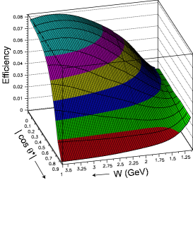
Figure 5: Two-dimensional dependence of the efficiency on ($W$, $|\cos\theta^{*}|$).

IV.4 Derivation of differential cross sections

The differential cross section for each ($W$, $|\cos\theta^{*}|$) point is given by:

$$\frac{d\sigma}{d|\cos\theta^{*}|}=\frac{\Delta Y}{\Delta W\Delta|\cos\theta^{*}|\int{\cal L}dt\ L_{\gamma\gamma}(W)\ \epsilon\ {\cal B}^{2}},$$ (2)

where $\Delta Y$ is the signal yield after the $\eta$-mass sideband subtraction, $\Delta W$ and $\Delta|\cos\theta^{*}|$ are the bin widths, $\int{\cal L}dt$ and $L_{\gamma\gamma}(W)$ are the integrated luminosity and two-photon luminosity function calculated with TREPS treps , respectively, $\epsilon$ is the efficiency, and ${\cal B}^{2}$ is the squared branching fraction for $\eta\to\gamma\gamma$. The over-subtraction of signal in the sideband due to the leakage of the signal into the sideband region is evaluated in the MC, separately, and finally included in the efficiency $\epsilon$.

The bin sizes $\Delta W$ and $\Delta|\cos\theta^{*}|$ and the maximum $|\cos\theta^{*}|$ for which we obtain the differential cross section are summarized in Table 2. We first derive the differential cross sections for bin widths of $\Delta W=0.02$ GeV and $\Delta|\cos\theta^{*}|=0.1$, and average the differential cross section over two or five different $W$ regions to obtain results for $\Delta W=0.04$ GeV or 0.10 GeV, respectively.

We do not give a cross section for $W>3.3$ GeV. In the $W$ range 3.3–3.6 GeV, the charmonium component dominates the yield, and we cannot subtract it in a model-independent way. We also cannot give the cross section including the charmonium contribution in these bins, because leakages from the narrow $\chi_{c0}$ peak around 3.41 GeV into adjacent bins due to energy resolution complicate the extraction of cross sections in each bin. Above $W>3.6$ GeV, we do not find any significant signal after consideration of the backgrounds.

Figure 6 shows the angular dependence of the differential cross sections for selected $W$ bins. Figure 7 shows the cross section integrated over $|\cos\theta^{*}|<0.9$ for the entire $W$ range and that for $|\cos\theta^{*}|<1.0$ in the range $W<2.0$ GeV.

Table 2: Bin sizes. The lowest bound of the first $W$ range (1.0957 GeV) corresponds to the mass threshold.

$W$ range	$\Delta W$	$\Delta|\cos\theta^{*}|$	maximum
(GeV)	(GeV)		$|\cos\theta^{*}|$
1.0957 – 1.12	0.0243	0.1	1.0
1.12 – 2.0	0.04	0.1	1.0
2.0 – 2.4	0.04	0.1	0.9
2.4 – 3.3	0.10	0.1	0.9

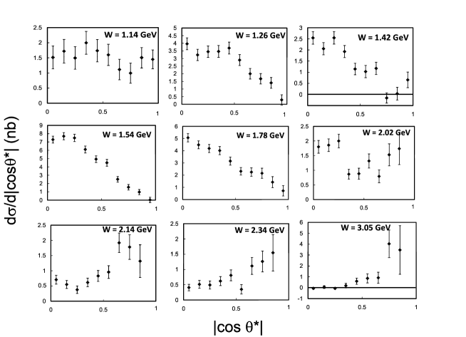
Figure 6: Angular dependence of the differential cross sections for nine selected $W$ bins indicated. The bin sizes are summarized in Table 2.

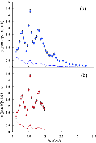
Figure 7: (a) The cross section integrated over $|\cos\theta^{*}|<0.9$ and (b) over $|\cos\theta^{*}|<1.0$ for $W<2.0$ GeV. Errors are statistical only. The dotted curve shows the size of the systematic uncertainty.

IV.5 Systematic errors

Various sources of systematic uncertainties assigned for the $\eta\eta$ signal yield, efficiency and the cross section evaluation are described in detail below and summarized in Table 3.

• Trigger efficiency: The systematic error due to uncertainty in the threshold for the Clst4 trigger ($\sim 110$ MeV) is very small, because photons from $\eta$ decays have high enough energy. However, the efficiency of the HiE trigger dominates that of Clst4 except in the lowest $W$ region, because the former has a looser condition for the number of clusters in the acceptance region of the trigger. We estimate the uncertainty in the efficiency for the HiE trigger to be 4% over the whole $W$ region, and treat it as the combined systematic error for the two kinds of triggers.

• $\eta$ selection efficiency: We assign 6% for the selection of the two $\eta$’s. This corresponds to a 3% uncertainty for the efficiency of each $\eta$ reconstruction.

• Overlapping hits from beam background and related effects: We assign a 4% (3%) error for $W<1.44$ GeV ($W>1.44$ GeV) for uncertainties of the inefficiency in event selection due to beam-background photons, which affect the photon multiplicity and $\eta$ reconstruction. The uncertainty is estimated by comparing efficiencies among different experimental periods and background conditions. We adopt the average efficiency from different background files, and the uncertainty in the average, obtained from the variation of experimental yield in different run periods, is assigned as the error.

• $p_{t}$-balance cut: A 3% uncertainty is assigned. The $p_{t}$-balance distribution for the signal is well reproduced by MC so that the efficiency is correct to within this error.

• Sideband background subtraction: 1/3 of the size of the subtracted component is assigned to this source for each bin. We conservatively assign this error because we ignore the non-linear behavior of the background in the $M_{\gamma\gamma}$ distribution in the sideband subtraction. This effect is expected to be large but cannot be determined precisely in the lowest $W$ bins.

• $p_{t}$-unbalanced background: We have applied a $-3\%$ correction for this background source only in the lowest and highest $W$ regions, $W<1.2$ GeV and $W>3.2$ GeV. We do not find any evidence of such a component, and no correction is applied for this effect in the other energies. We assign a 2% error from this source for the entire $W$ region.

• Luminosity function: We assign 4% (5%) for $W$ below (above) 3.0 GeV; this includes the uncertainties in the equivalent photon approximation (3% (4%)), the radiative corrections that were neglected (1-2%) and the integrated luminosity (1.4%).

• No unfolding:

  Uncertainty from smearing effects is estimated by smearing a modeled resonance function with the $W$ resolution and examining apparent changes of the cross section. The changes are large ($\sim 7\%$) only near the slopes of the narrowest resonant structure, in the region $1.44~{}{\rm GeV}\leq W\leq 1.60~{}{\rm GeV}$, and smaller (4%) in other $W$ ranges.

• Other efficiency errors: An error of 4% is assigned for uncertainties in the efficiency determination based on MC including the smoothing procedure.

The total systematic error is obtained by adding all the sources in quadrature and is 11–12% for the intermediate and high $W$ regions. It becomes more than 20% for $W<1.24~{}{\rm GeV}$.

In the resonance analyses for $W<2.0$ GeV in Sec. V, we treat the systematic error sources except for (9) as uncertainties in the overall normalization, which are correlated in the different ($W$, $|\cos\theta^{*}|$) bins. For the analysis of the $W$ dependence in the high energy region (Sec. VI.B), we also take into account energy-dependent deviations for sources (6) and (8).

Table 3: Systematic errors for the differential cross sections. Ranges of errors are shown when they depend on $W$.

Source	Error (%)
Trigger efficiency	4
$\eta$-pair reconstruction efficiency	6
Overlapping hits from beam background etc.	3 – 4
$p_{t}$-balance cut	3
Sideband background subtraction	2 – 27 (for $W$>1.2 GeV)
	28 – 60 (for $W$<1.2 GeV)
$p_{t}$-unbalanced background subtraction	2
Luminosity function and integrated luminosity	4 – 5
Unfolding	4 – 7
Other efficiency errors	4
Overall	11 – 29 (for $W>1.2~{}{\rm GeV}$)
	30 – 61 (for $W<1.2~{}{\rm GeV}$)

V Study of resonances

In the total cross section (Fig. 7), clear peaks due to the $f_{2}(1270)$ and $f_{2}^{\prime}(1525)$ are visible along with other possible resonances. In this section, we first present consistency checks with previous measurements and report improved measurements of some of these resonances.

V.1 Differential Cross Sections in Partial Waves

In the energy region $W\leq 3~{}{\rm GeV}$, $J>4$ partial waves (next is $J=6$) may be neglected so that only S, D and G waves are considered. The differential cross section can be expressed as:

$$\frac{d\sigma}{d\Omega}(\gamma\gamma\to\eta\eta) = \left|S\>Y^{0}_{0}+D_{0}\>Y^{0}_{2}+G_{0}\>Y^{0}_{4}\right|^{2}$$ (3)

$$+ \left|D_{2}\>Y^{2}_{2}+G_{2}\>Y^{2}_{4}\right|^{2},$$

where $D_{0}$ and $G_{0}$ ($D_{2}$ and $G_{2}$) denote the helicity 0 (2) components of the D and G waves, respectively, and $Y^{\lambda}_{J}$ are the spherical harmonics in which the helicity $\lambda$ is quantized along the $\gamma\gamma$ axis. Since the $|Y^{\lambda}_{J}|$’s are not independent of each other partial waves cannot be separated from the information in the differential cross sections alone.

We rewrite Eq. (3) as

$$\frac{d\sigma}{4\pi d|\cos\theta^{*}|}(\gamma\gamma\to\eta\eta) =$$

$$\hat{S}^{2}|Y^{0}_{0}|^{2}+\hat{D}_{0}^{2}|Y^{0}_{2}|^{2} + \hat{D}_{2}^{2}|Y^{2}_{2}|^{2}$$

$$+\hat{G}_{0}^{2}|Y^{0}_{4}|^{2}+\hat{G}_{2}^{2}|Y^{2}_{4}|^{2}$$ . (4)

The amplitudes $\hat{S}^{2}$, $\hat{D}_{0}^{2}$, $\hat{D}_{2}^{2}$, $\hat{G}_{0}^{2}$ and $\hat{G}_{2}^{2}$ can be expressed in terms of $S$, $D_{0}$, $D_{2}$, $G_{0}$ and $G_{2}$ pi0pi0 . Since the square of spherical harmonics are independent of each other, we can fit differential cross sections to obtain $\hat{S}^{2}$, $\hat{D}_{0}^{2}$, $\hat{D}_{2}^{2}$, $\hat{G}_{0}^{2}$ and $\hat{G}_{2}^{2}$ in each $W$ bin. Since $|Y^{0}_{4}|^{2}$ and $|Y^{2}_{4}|^{2}$ are nearly equal for $|\cos\theta^{*}|<0.7$ we also fit $\hat{G}_{0}^{2}+\hat{G}_{2}^{2}$ and $\hat{G}_{0}^{2}-\hat{G}_{2}^{2}$. Two types of fits are made: the “SD” fit and “SDG” fit. G waves are neglected in the SD fit.

The spectra of $\hat{S}^{2}$, $\hat{D}_{0}^{2}$ and $\hat{D}_{2}^{2}$ obtained for the SD fit and $\hat{G}_{0}^{2}$, $\hat{G}_{2}^{2}$ and $\hat{G}_{0}^{2}\pm\hat{G}_{2}^{2}$ for the SDG fit are shown in Figs. 8 and 9. The spectra of $\hat{S}^{2}$, $\hat{D}_{0}^{2}$ and $\hat{D}_{2}^{2}$ for the SDG fit are omitted because they are nearly the same as those for the SD fit with somewhat larger statistical errors. It appears that the D₀ and G waves are small enough to be neglected in the region of interest ($W<2.0~{}{\rm GeV})$. In that case, $\hat{S}^{2}$ and $\hat{D}_{2}^{2}$ become $|S|^{2}$ and $|D_{2}|^{2}$, respectively, which simplifies the parameterization. In the fits performed here, we neglect the G waves completely, and take $D_{0}=0$ in the nominal fit.

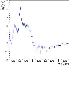
Figure 8: Spectra of $\hat{S}^{2}$, $\hat{D}_{0}^{2}$ and $\hat{D}_{2}^{2}$ for the SD fit. Those for the SDG fit are nearly identical with larger statistical errors. The error bars shown are statistical errors that do not include correlations.

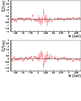
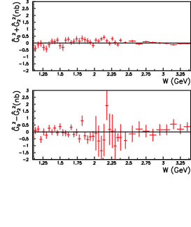
Figure 9: Spectra of $\hat{G}_{0}^{2}$ and $\hat{G}_{2}^{2}$ and $\hat{G}_{0}^{2}\pm\hat{G}_{2}^{2}$. The error bars shown are statistical errors that do not include correlations.

V.2 Fitting Partial Wave Amplitudes

In this subsection, we describe the extraction of resonant substructure by fitting differential cross sections by parameterizing partial wave amplitudes in terms of resonances and smooth “backgrounds”. Note that we do not fit $\hat{S}^{2}$, $\hat{D}_{0}^{2}$ and $\hat{D}_{2}^{2}$, but instead fit the differential cross sections directly. Once the functional forms of amplitudes are assumed, we can use Eq. (3) to fit differential cross sections. We then do not have to worry about the correlations between $\hat{S}^{2}$, $\hat{D}_{0}^{2}$ and $\hat{D}_{2}^{2}$. The $\hat{S}^{2}$, $\hat{D}_{0}^{2}$ and $\hat{D}_{2}^{2}$ spectra are compared with the results of parameterization. Here we neglect the D₀ and G waves in the fitting region, $W<2.00~{}{\rm GeV}$.

Quite a few resonances are listed in Ref. PDG (PDG) that are known to decay into $\eta\eta$ with measured or unknown branching fractions to two photons. Besides the $f_{2}(1270)$ and $f_{2}^{\prime}(1525)$, there are $f_{2}(1565)$, $f_{2}(1910)$ and $f_{2}(1950)$ tensor mesons, $f_{0}(1370)$, $f_{0}(1500)$, $f_{0}(1710)$ and $f_{0}(2020)$ scalar mesons, and spin-4 $f_{4}(2050)$ states. So far quantitative measurements of the branching fraction to $\eta\eta$ based on observed enhancements in mass spectra are available for $f_{2}(1270)$ gams ; wa102 and $f^{\prime}_{2}(1525)$ gams2 . In addition, a phenomenological derivation of the $\eta\eta$ branching fraction based on a K-matrix approach kmat has been tried for the $f^{\prime}_{2}(1525)$ PDG .

To investigate this complicated region, we divide our analysis into two parts. First, we try to confirm or improve the parameter $\Gamma_{\gamma\gamma}{\cal B}(\eta\eta)$ of the well established tensor mesons, $f_{2}(1270)$ and $f_{2}^{\prime}(1525)$, by fitting in the region $W<1.64$ GeV. We then investigate the higher mass region by fixing most of the parameters in the fit from results in the low mass region.

V.2.1 Low mass region, 1.12 – 1.64 GeV

We concentrate on the resonances, $f_{2}(1270)$ and $f_{2}^{\prime}(1525)$ by fitting the region $W<1.64~{}{\rm GeV}$. The resonances taken into account are the $f_{2}(1270)$, $f_{2}^{\prime}(1525)$ and “$f_{0}(Y)$”, where “$f_{0}(Y)$” is just a parameterization motivated by the $f_{0}(1370)$ and $f_{0}(1500)$. We parameterize partial waves as follows:

$$S = A_{f_{0}(Y)}e^{i\phi_{Y}}+B_{S}e^{i\phi_{s}},$$

$$D_{0} = B_{D0},$$

$$D_{2} = A_{f_{2}(1270)}e^{i\phi_{2}}+A_{f_{2}^{\prime}(1525)}e^{i\phi_{5}}+B_{D2},$$

where $A_{f_{0}(Y)}$, $A_{f_{2}(1270)}$ and $A_{f_{2}^{\prime}(1525)}$ are the amplitudes of the corresponding resonances; $B_{S}$, $B_{D0}$ and $B_{D2}$ are “background” amplitudes for $S$, $D_{0}$ and $D_{2}$ waves; $\phi_{Y}$, $\phi_{2}$ and $\phi_{5}$ are the phases of resonances relative to background amplitudes; $\phi_{s}$ is the relative phase between $S$ and $D_{0}$. We set $B_{D0}=0$ (and then $\phi_{s}=0$) for simplicity in the nominal fit, but we later consider a non-zero $D_{0}$ contribution to determine the systematic errors for the obtained resonance parameters and leave the $B_{D0}$ symbol here.

To parameterize resonances, we use a relativistic Breit-Wigner amplitude $A_{R}(W)$ for each spin-$J$ resonance $R$ of mass $m_{R}$ given by

$$A_{R}^{J}(W) = \sqrt{\frac{8\pi(2J+1)m_{R}}{W}}$$

$$\times \frac{\sqrt{\Gamma_{\rm tot}(W)\Gamma_{\gamma\gamma}(W){\cal B}(R\rightarrow\eta\eta)}}{m_{R}^{2}-W^{2}-im_{R}\Gamma_{\rm tot}(W)}\;.$$

For scalar mesons, partial and total widths do not depend on $W$, while for tensor mesons (the $f_{2}(1270)$ and $f_{2}^{\prime}(1525)$, $f_{2}(1810)$ and $f_{2}(1950)$), the energy-dependent total width $\Gamma_{\rm tot}(W)$ is given by

$$\Gamma_{\rm tot}(W)=\sum_{X}\Gamma_{X\bar{X}}(W)\;,$$ (7)

where $X$ is a $\pi$, $K$, $\eta$, $\gamma$, etc. The partial width $\Gamma_{X\bar{X}}(W)$ is parameterized as blat :

$$\Gamma_{X\bar{X}}(W) = \Gamma_{R}{\cal B}(R\rightarrow X\bar{X})\left(\frac{q_{X}(W^{2})}{q_{X}(m_{R}^{2})}\right)^{5}$$ (8)

$$\times \frac{D_{2}\left(q_{X}(W^{2})r_{R}\right)}{D_{2}\left(q_{X}(m_{R}^{2})r_{R}\right)}\;,$$

where $\Gamma_{R}$ is the total width at the resonance mass, $q_{X}(W^{2})=\sqrt{W^{2}/4-m_{X}^{2}}$, $D_{2}(x)=1/(9+3x^{2}+x^{4})$, and $r_{R}$ is an effective interaction radius that varies from 1 ${\rm GeV}^{-1}$ to 7 ${\rm GeV}^{-1}$ in different hadronic reactions grayer . We assume the same $r_{R}$ value from Ref. mori2 for the $f_{2}(1270)$ and $f^{\prime}_{2}(1525)$.

For the $4\pi$ and other decay modes, $\Gamma_{4\pi}(W)=\Gamma_{R}{\cal B}(R\rightarrow 4\pi)\frac{W^{2}}{m_{R}^{2}}$ is used instead of Eq. (8) for the $f_{2}(1270)$. Parameters of the $f_{2}(1270)$ and $f_{2}^{\prime}(1525)$ are summarized in Table 4. The resonance parameters given in Ref. PDG for the $f_{0}(1370)$ and $f_{0}(1500)$ are summarized in Table 5. Background amplitudes are parameterized as follows.

$$B_{S} = \beta(b_{S}(W-W_{0})+c_{S}),$$

$$B_{D0} = \beta^{5}(b_{0}(W-W_{0})+c_{0}),$$

$$B_{D2} = \beta^{5}(b_{2}(W-W_{0})+c_{2}),$$

where $\beta$ is the velocity of the $\eta$ meson in the c.m.s. and $W_{0}=2m_{\eta}$. We set $B_{D0}=0$, that is, $b_{0}=c_{0}=0$, in the nominal fit. We assume the background amplitudes for $S$ and $D_{2}$ to be real and linear in $W$ to reduce the number of parameters. Furthermore, we fix arbitrary phases by choosing $c_{S}>0$, and $c_{2}>0$.

We fit the energy region of $1.12~{}{\rm GeV}<W<1.64~{}{\rm GeV}$. In the fit, we fix the values of the parameters of the $f_{2}(1270)$ and $f_{2}^{\prime}(1525)$ to those in the PDG PDG except for the product $\Gamma_{\gamma\gamma}{\cal B}(\eta\eta)$ for the $f_{2}(1270)$.

Two hundred sets of randomly generated initial parameters are prepared and fits are performed for each study. A unique solution is obtained with a fit quality of $\chi^{2}/ndf=137.1/119$, where $ndf$ is the number of degrees of freedom in the fit. A fit without $f_{0}(Y)$ gives a poor fit with $\chi^{2}/ndf=209.7/123$. The parameters obtained from these two fits are summarized in Table LABEL:tab:fit1. The product $\Gamma_{\gamma\gamma}{\cal B}(\eta\eta)$ for the $f_{2}(1270)$ is $11.5^{+1.8}_{-2.0}$ eV and is consistent with $12.1\pm 2.8$ eV in PDG PDG . Figures 10 to 12 show results of the nominal fit to differential cross sections, the total cross section, and spectra of $\hat{S}^{2}$, $\hat{D}_{0}^{2}$ and $\hat{D}_{2}^{2}$.

Fits where the value of the product $\Gamma_{\gamma\gamma}{\cal B}(\eta\eta)$ of the $f_{2}^{\prime}(1525)$ is floated while that of the $f_{2}(1270)$ is fixed to the PDG value, yields three solutions listed in Table 7. Thus we fix the former to the PDG values in further studies.

The following sources of systematic errors on the parameters are considered: dependence on the fitted region, normalization errors of the differential cross sections, assumptions on the background amplitudes, and the measurement errors of the $f_{2}(1270)$ and $f^{\prime}_{2}(1525)$.

For each study, a fit is made allowing all the parameters to float; the differences of the fitted parameters from the nominal values are quoted as systematic errors. Here too, two hundred sets of randomly generated initial parameters are prepared for each study and fitted to search for the true minimum and for possible multiple solutions. Unique solutions are found many times. Once a solution is found, several more iterations of the fitting procedure are made to confirm the convergence.

The resulting systematic errors are summarized in Table 8. Two fitting regions are tried: one region that is shifted lower by one bin ($1.08~{}{\rm GeV}\leq W\leq 1.60~{}{\rm GeV}$) and another shifted higher by one bin ($1.16~{}{\rm GeV}\leq W\leq 1.68~{}{\rm GeV}$). Studies on normalization are divided into those from uncertainties of the overall normalization and those from distortion of the spectra in either $|\cos\theta^{*}|$ or $W$. For overall normalization errors, fits are made with two sets of values of differential cross sections obtained by multiplying by $(1\pm\sigma_{\epsilon}(W,|\cos\theta^{*}|))$, where $\sigma_{\epsilon}$ is the relative efficiency error; they are denoted as “normalization$\pm$” in the table. For distortion studies, $\pm 4$% errors for $|\cos\theta^{*}|<1$ and $\pm 4$%/GeV for the $W$ dependence are assigned, based on the uncertainty discussed for (9) in Sec. IV.E. Differential cross sections are modified by multiplying by $(1\pm 0.08|\cos\theta^{*}|\mp 0.04)$ and $(1\pm 0.08(W{\rm[GeV]}-1.38))$ (denoted as “bias:$|\cos\theta^{*}|\pm$” and “bias:$W\pm$”, respectively). For studies of background (BG) amplitudes, either $b_{i}$ or $c_{i}$ is set to zero for $B_{S}$ and $B_{D2}$, while either $b_{0}$ or $c_{0}$ is floated for $B_{D0}$. Finally, the parameters of the $f_{2}(1270)$, $f_{2}^{\prime}(1525)$, and the value of $r_{R}$ are successively varied by their errors.

The total systematic errors are calculated by adding individual errors in quadrature. As can be seen in Table 8, we obtain

$$\Gamma_{\gamma\gamma}{\cal B}(f_{2}(1270)\to\eta\eta)=11.5~{}^{+1.8}_{-2.0}~{}^{+4.5}_{-3.7}~{}{\rm eV},$$ (9)

which is consistent with previous measurements PDG . The apparent threshold enhancement in the S wave is fitted in terms of a scalar meson, $f_{0}(Y)$ whose mass, width and $\Gamma_{\gamma\gamma}{\cal B}(\eta\eta)$ are obtained to be

$$M_{f_{0}(Y)}=1262^{+51}_{-78}~{}^{+82}_{-103}~{}{\rm MeV}/c^{2},$$

$$\Gamma_{f_{0}(Y)}=484~{}^{+246}_{-170}~{}^{+246}_{-263}~{}{\rm MeV},$$

$$\Gamma_{\gamma\gamma}{\cal B}(f_{0}(Y)\to\eta\eta)=121~{}^{+133}_{-53}~{}^{+169}_{-106}~{}{\rm eV},$$

(12)

respectively.

The mass peak of the $f_{0}(Y)$ does not coincide with the broad peak in the $\hat{S}^{2}$ spectrum in Fig. 12 due to the effects of interference.

Table 4: Parameters of the $f_{2}\left(1270\right)$ and $f_{2}^{\prime}\left(1525\right)$ assumed or fitted in Ref. mori2 .

Parameter	$f_{2}\left(1270\right)$	$f_{2}^{\prime}\left(1525\right)$	Unit	Reference
Mass	$1275.1\pm 1.2$	$1525\pm 5$	${\rm MeV}/c^{2}$	PDG
Width	$185.1^{+2.9}_{-2.4}$	$73^{+6}_{-5}$	MeV	PDG
${\cal B}({f_{2}\rightarrow\pi\pi})$	$(84.8^{+2.4}_{-1.2})\%$	$(0.82\pm 0.15)\%$		PDG
${\cal B}({f_{2}\rightarrow K\bar{K}})$	$(4.6\pm 0.4)\%$	$(88.7\pm 2.2)\%$		PDG
${\cal B}({f_{2}\rightarrow\eta\eta})$	$(4.0\pm 0.8)\times 10^{-3}$	$(10.4\pm 2.2)\%$		PDG
${\cal B}({f_{2}\rightarrow\gamma\gamma})$	$(1.64\pm 0.19)\times 10^{-5}$	$(1.11\pm 0.14)\times 10^{-6}$		PDG
$r_{R}$	$3.62\pm 0.03$	$3.62\pm 0.03$	$({\rm GeV}/c)^{-1}$	mori2

Table 5: Parameters of the $f_{0}(1370)$ and $f_{0}(1500)$ PDG .

Parameter	$f_{0}(1370)$	$f_{0}(1500)$	Unit
Mass	1200 – 1500	$1505\pm 6$	MeV/$c^{2}$
Width	150 – 250	$109\pm 7$	MeV
${\cal B}(\eta\eta)$	seen	$(5.1\pm 0.9)\%$
${\cal B}(\gamma\gamma)$	unknown	unknown

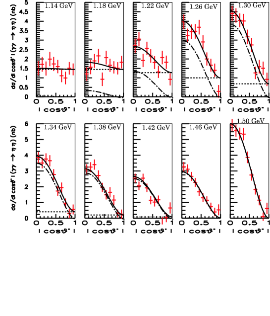
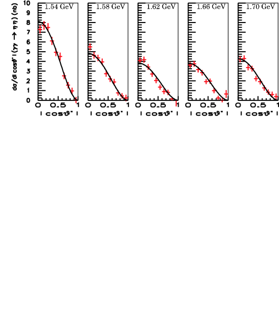
Figure 10: Differential cross sections (points with error bars) and fitted curves for the nominal fit in the low mass region (solid curve). Dotted (dot-dashed) curves are $|S|^{2}$ ($|D_{2}|^{2}$) from the fit. The vertical error bars are statistical only.

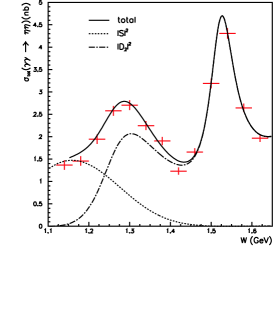
Figure 11: Total cross section (points with error bars) ($|\cos\theta^{*}|<1.0$) and fitted curves for the nominal fit in the low mass region (solid curve). Dotted (dot-dashed) curves are $|S|^{2}$ ($|D_{2}|^{2}$) from the fit. The vertical errors are statistical only.

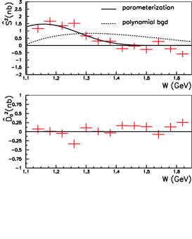
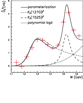
Figure 12: $\hat{S}^{2}$, $\hat{D}_{0}^{2}$ and $\hat{D}_{2}^{2}$ and fitted curves for the nominal fit in the low mass region (solid curve). The points with error bars are the results of the $W$-independent fits (same as those in Fig. 8). The vertical error bars are statistical only.

Table 6: Fitted parameters for the nominal fit and for a fit without the $f_{0}(Y)$ in the low mass region.

Parameter	Nominal	Without $f_{0}(Y)$	Unit
Mass $(f_{0}(Y))$	$1262^{+51}_{-78}$	–	${\rm MeV}/c^{2}$
Width $(f_{0}(Y))$	$484^{+246}_{-170}$	–	${\rm MeV}$
$\Gamma_{\gamma\gamma}{\cal B}(\eta\eta)(f_{0}(Y))$	$121^{+133}_{-53}$	0 (fixed)	eV
$\phi_{Y}$	$38^{+19}_{-30}$	–	deg.
$\Gamma_{\gamma\gamma}{\cal B}(\eta\eta)(f_{2}(1270))$	$11.5^{+1.8}_{-2.0}$	$11.7^{+1.4}_{-1.5}$	eV
$\phi_{2}$	$68^{+7}_{-5}$	$66\pm 4$	deg.
$\phi_{5}$	$150^{+14}_{-12}$	$164\pm 13$	deg.
$b_{S}$	$-2.9^{+3.2}_{-3.5}$	$-8.5^{+0.3}_{-0.4}$	$\sqrt{\rm nb/GeV}$
$c_{S}$	$2.3^{+2.3}_{-1.8}$	$3.7\pm 0.1$	$\sqrt{\rm nb}$
$b_{2}$	$6.5^{+7.6}_{-5.7}$	$-3.9^{+3.6}_{-4.5}$	$\sqrt{\rm nb/GeV}$
$c_{2}$	$1.8^{+3.5}_{-4.6}$	$6.9^{+3.0}_{-2.3}$	$\sqrt{\rm nb}$
$\chi^{2}\;(ndf)$	137.1 (119)	209.7 (123)	–

Table 7: Three solutions obtained when $\Gamma_{\gamma\gamma}{\cal B}(\eta\eta)(f_{2}^{\prime}(1525))$ is floated in fits to the low mass region.

Parameter	Sol.A	Sol. B	Sol. C	Unit
Mass $(f_{0}(Y))$	$1259^{+50}_{-79}$	$1259^{+54}_{-80}$	$1264^{+55}_{-86}$	${\rm MeV}/c^{2}$
Width $(f_{0}(Y))$	$471^{+234}_{-169}$	$502^{+241}_{-191}$	$536^{+261}_{-193}$	${\rm MeV}$
$\Gamma_{\gamma\gamma}{\cal B}(\eta\eta)(f_{0}(Y))$	$116^{+122}_{-52}$	$127^{+139}_{-59}$	$143^{+162}_{-69}$	eV
$\phi_{Y}$	$36^{+20}_{-31}$	$38^{+19}_{-32}$	$41^{+18}_{-30}$	deg.
$\Gamma_{\gamma\gamma}{\cal B}(\eta\eta)(f_{2}^{\prime}(1525))$	$23.1^{+2.6}_{-2.8}$	$8.0^{+2.0}_{-1.5}$	$5.0^{+5.8}_{-5.0}$	eV
$\phi_{2}$	$4^{+10}_{-9}$	$68^{+10}_{-11}$	$45^{+23}_{-21}$	deg.
$\phi_{5}$	$188^{+17}_{-14}$	$155^{+10}_{-11}$	$94\pm 22$	deg.
$b_{S}$	$-2.9^{+3.2}_{-3.7}$	$-2.9^{+3.2}_{-3.7}$	$-2.9^{+3.2}_{-3.6}$	$\sqrt{\rm nb/GeV}$
$c_{S}$	$2.3^{+2.4}_{-1.9}$	$2.3^{+1.7}_{-1.9}$	$2.4^{+2.6}_{-1.9}$	$\sqrt{\rm nb}$
$b_{2}$	$1.5^{+6.0}_{-4.8}$	$3.8^{+6.4}_{-1.9}$	$-12.5^{+2.5}_{-2.4}$	$\sqrt{\rm nb/GeV}$
$c_{2}$	$5.2^{+2.8}_{-3.2}$	$3.2\pm 1.2$	$5.8^{+1.1}_{-1.2}$	$\sqrt{\rm nb}$
$\chi^{2}\;(ndf)$	136.4 (119)	137.2 (119)	138.6 (119)	–

Table 8: Systematic uncertainties for the fit in the low mass region.

	$f_{0}(Y)$			$f_{2}(1270)$
Source	Mass	$\Gamma_{\rm tot}$	$\Gamma_{\gamma\gamma}{\cal B}(\eta\eta)$	$\Gamma_{\gamma\gamma}{\cal B}_{\eta\eta}$
	(MeV/$c^{2}$)	(MeV)	(eV)	(eV)
$W$ range	${}^{+56.5}_{-8.9}$	${}^{+0.0}_{-17.8}$	${}^{+26.9}_{-17.0}$	${}^{+0.4}_{-1.1}$
Bias:$W$	${}^{+1.1}_{-1.7}$	${}^{+1.2}_{0.0}$	${}^{+2.3}_{-2.1}$	${}^{+0.1}_{-0.1}$
Bias:$|\cos\theta^{*}|$	${}^{+0.1}_{-0.5}$	${}^{+0.5}_{-0.8}$	${}^{+0.6}_{-0.9}$	${}^{+0.1}_{-0.1}$
Normalization	${}^{+27.0}_{-48.8}$	${}^{+220.9}_{-199.1}$	${}^{+152.1}_{-87.1}$	${}^{+3.0}_{-2.4}$
BG:$B_{S}$	${}^{+0.0}_{-84.9}$	${}^{+0.0}_{-162.9}$	${}^{+0.0}_{-54.3}$	${}^{+0.7}_{-0.0}$
BG:$D_{0}$	${}^{+49.6}_{-0.0}$	${}^{+0.0}_{-42.1}$	${}^{+57.3}_{-0.0}$	${}^{+0.0}_{-2.0}$
BG:$D_{2}$	${}^{+4.6}_{-10.1}$	${}^{+100.1}_{-26.7}$	${}^{+30.4}_{-6.0}$	${}^{+1.9}_{-0.8}$
$f_{2}$ mass	${}^{+0.4}_{-0.2}$	${}^{+4.1}_{-2.5}$	${}^{+2.0}_{-1.4}$	${}^{+0.3}_{-0.3}$
$f_{2}$ width	${}^{+1.1}_{-0.4}$	${}^{+0.4}_{-0.0}$	${}^{+1.3}_{-0.5}$	${}^{+0.2}_{-0.2}$
$f_{2}^{\prime}$ mass	${}^{+8.7}_{-24.7}$	${}^{+41.5}_{-0.0}$	${}^{+21.1}_{-20.3}$	${}^{+2.2}_{-1.4}$
$f_{2}^{\prime}$ width	${}^{+4.8}_{-5.6}$	${}^{+2.5}_{-8.4}$	${}^{+0.5}_{-2.7}$	${}^{+0.3}_{-0.4}$
$f_{2}^{\prime}\;\Gamma_{\gamma\gamma}{\cal B}(\eta\pi^{0})$	${}^{+13.0}_{-13.7}$	${}^{+11.7}_{-0.0}$	${}^{+13.0}_{-6.6}$	${}^{+1.5}_{-0.4}$
$r_{R}$	${}^{+0.2}_{-0.2}$	${}^{+0.6}_{-1.5}$	${}^{+0.2}_{-0.4}$	${}^{+0.0}_{-0.0}$
Total	${}^{+81.7}_{-103.0}$	${}^{+246.4}_{-262.8}$	${}^{+169.4}_{-106.4}$	${}^{+4.5}_{-3.7}$

V.2.2 Higher mass region, up to 2.0 GeV

Now we investigate the higher mass region. We fix most of parameters determined at lower energy, and introduce, just for the purpose of parameterization, a single tensor resonance, $f_{2}(X)$, whose mass, width and $\Gamma_{\gamma\gamma}{\cal B}(\eta\eta)$ are left free and fit the region $1.16~{}{\rm GeV}<W<2.0~{}{\rm GeV}$. We parameterize partial waves as follows:

$$S = A_{f_{0}(Y)}e^{i\phi_{Y}}+B_{S}e^{i\phi_{s}},$$

$$D_{0} = B_{D0},$$

$$D_{2} = A_{f_{2}(1270)}e^{i\phi_{2}}+A_{f_{2}^{\prime}(1525)}e^{i\phi_{5}}$$

$$+A_{f_{2}(X)}e^{i\phi_{X}}+B_{D2},$$

where $A_{f_{0}(Y)}$, $A_{f_{2}(1270)}$ and $A_{f_{2}^{\prime}(1525)}$, are fixed at the values that are fitted in the low mass region. Here too, $B_{D0}$ is set to zero and $B_{S}$ is fixed at the values found above. The phases $\phi_{Y}$, $\phi_{2}$ and $\phi_{5}$ are also fixed and $\phi_{s}=0$. Only the $b_{2}$ and $c_{2}$ parameters of $B_{D2}$ are floated along with the parameters of $f_{2}(X)$, i.e., its mass, width, $\Gamma_{\gamma\gamma}{\cal B}(\eta\eta)$ and $\phi_{X}$.

Two hundred sets of randomly generated initial parameters are prepared and fits are performed for each study. A unique solution is obtained with a fit quality of $\chi^{2}/ndf=311.4/204$. The parameters obtained are summarized in Table 9. Figures 13 to 15 show results of the nominal fit to the differential cross sections, the total cross section, and spectra of $\hat{S}^{2}$, $\hat{D}_{0}^{2}$ and $\hat{D}_{2}^{2}$. A more sophisticated parameterization results in multiple solutions. As an example, two solutions are found when the parameters of $B_{S}$ are also floated; these are also listed in Table 9. Hence we employ the simple parameterization given in Eq. (13). This parameterization results in discrepancies from the fits in some $W$ regions for differential and integrated cross sections.

Various sources of the systematic errors are studied and evaluated using various fits similar to those applied in the analysis for the low mass region, as summarized in Table 10. We take into account the errors for the $f_{0}(Y)$ parameters, as well as those for $f_{2}(1270)$ and $f^{\prime}_{2}(1525)$. We try two fitting regions shifted lower by two bins ($1.08~{}{\rm GeV}\leq W\leq 1.92~{}{\rm GeV}$) and higher by two bins ($1.24~{}{\rm GeV}\leq W\leq 2.08~{}{\rm GeV}$). For studies of background (BG) amplitudes, either $c_{2}$ or $b_{2}$ is set to zero for $B_{D2}$ or allowed to float for $B_{D0}$. Values of $c_{S}$ and $b_{S}$ are changed by their errors.

The total systematic errors are calculated by adding the individual errors in quadrature. The mass, width and $\Gamma_{\gamma\gamma}{\cal B}(\eta\eta)$ obtained for the $f_{2}(X)$ meson are

$$M_{f_{2}(X)}=1737~{}\pm 9~{}^{+198}_{-65}~{}{\rm MeV}/c^{2},$$ (14)

$$\Gamma_{f_{2}(X)}=228~{}^{+21}_{-20}~{}^{+234}_{-153}~{}{\rm MeV},$$ (15)

$$\Gamma_{\gamma\gamma}{\cal B}(f_{2}(X)\to\eta\eta)=5.2~{}^{+0.9}_{-0.8}~{}^{+37.3}_{-4.5}~{}{\rm eV},$$

(16)

respectively.

The rather poor $\chi^{2}$ of the fit and the clear disagreement in Figs. 14 and 15 above the $f^{\prime}_{2}(1525)$ may imply that more than one tensor resonance exists in this mass region. Unfortunately, we cannot draw any definite conclusions about such a possibility from additional fits to the data, because interference between amplitudes introduces too much additional freedom.

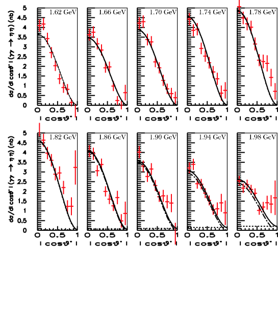
Figure 13: Differential cross sections (points with error bars) in the energy bins indicated and fitted curves for the nominal fit in the high mass region (solid curve). Dotted (dot-dashed) curves are $|S|^{2}$ ($|D_{2}|^{2}$) from the fit. The vertical error bars are statistical only.

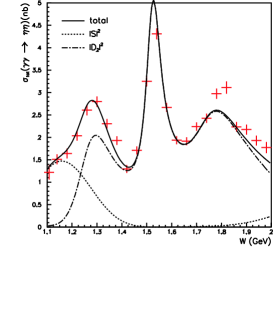
Figure 14: Total cross sections (points with error bars) ($|\cos\theta^{*}|<1.0$) and fitted curves for the nominal fit in the high mass region (solid curve). Dotted (dot-dashed) curves are $|S|^{2}$ ($|D_{2}|^{2}$) from the fit. The vertical error bars are statistical only.

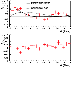
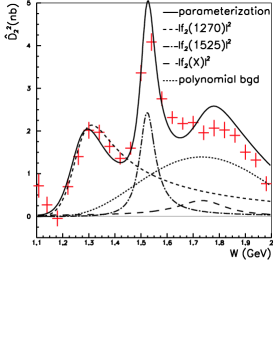
Figure 15: $\hat{S}^{2}$, $\hat{D}_{0}^{2}$ and $\hat{D}_{2}^{2}$ and fitted curves for the nominal fit in the high mass region (solid curve). The points with error bars are the results of the $W$-independent fits (same as those in Fig. 8). The vertical error bars are statistical only.

Table 9: Fitted parameters for the nominal fit and results obtained when the $B_{S}$ parameters are floated for the high mass region.

Parameter	Nominal	Free $B_{S}$		Unit
		Sol. A	Sol. B
Mass $(f_{2}(X))$	$1737\pm 9$	$1742\pm 10$	$1738\pm 9$	${\rm MeV}/c^{2}$
Width $(f_{2}(X))$	$228^{+21}_{-20}$	$223^{+23}_{-22}$	$236^{+21}_{-20}$	${\rm MeV}$
$\Gamma_{\gamma\gamma}{\cal B}(\eta\eta)(f_{2}(X))$	$5.2^{+0.9}_{-0.8}$	$4.7^{+1.0}_{-0.9}$	$6.0^{+1.2}_{-1.0}$	eV
$\phi_{X}$	$159^{+6}_{-5}$	$160^{+7}_{-6}$	$154\pm 5$	deg.
$b_{S}$	$-2.9$ (fixed)	$4.4\pm 0.3$	$-2.8\pm 0.3$	$\sqrt{\rm nb/GeV}$
$c_{S}$	2.3 (fixed)	$0.9\pm 0.2$	$1.8\pm 0.2$	$\sqrt{\rm nb}$
$b_{2}$	$-8.1\pm 0.7$	$-9.1^{+0.8}_{-0.9}$	$-9.9\pm 0.9$	$\sqrt{\rm nb/GeV}$
$c_{2}$	$9.4\pm 0.5$	$9.8^{+0.6}_{-0.5}$	$10.4\pm 0.6$	$\sqrt{\rm nb}$
$\chi^{2}\;(ndf)$	311.4 (204)	279.3 (202)	288.8 (202)	–

Table 10: Systematic uncertainties for the fit in the high mass region

	$f_{2}(X)$
Source	Mass	$\Gamma_{\rm tot}$	$\Gamma_{\gamma\gamma}{\cal B}(\eta\eta)$
	(MeV/$c^{2}$)	(MeV)	(eV)
$W$-range	${}^{+95.0}_{-0.0}$	${}^{+38.8}_{-101.8}$	${}^{+3.4}_{-1.5}$
Bias:$W$	${}^{+3.8}_{-3.8}$	${}^{+14.2}_{-13.0}$	${}^{+0.6}_{-0.5}$
Bias:$|\cos\theta^{*}|$	${}^{+0.7}_{-0.8}$	${}^{+6.1}_{-6.1}$	${}^{+0.4}_{-0.3}$
Normalization	${}^{+125.5}_{-10.4}$	${}^{+142.7}_{-0.0}$	${}^{+16.7}_{-0.0}$
BG:$c_{S}$	${}^{+0.0}_{-0.0}$	${}^{+0.0}_{-0.0}$	${}^{+0.0}_{-0.0}$
BG:$b_{S}$	${}^{+0.0}_{-0.0}$	${}^{+0.0}_{-0.0}$	${}^{+0.0}_{-0.0}$
BG:$B_{D0}$	${}^{+0.0}_{-1.4}$	${}^{+0.0}_{-6.2}$	${}^{+0.0}_{-0.5}$
$f_{2}$ mass	${}^{+1.0}_{-1.1}$	${}^{+4.7}_{-4.8}$	${}^{+0.2}_{-0.2}$
$f_{2}$ width	${}^{+1.1}_{-1.4}$	${}^{+5.1}_{-4.1}$	${}^{+0.2}_{-0.2}$
$f_{2}$ $\Gamma_{\gamma\gamma}{\cal B}(\eta\eta)$	${}^{+0.0}_{-8.2}$	${}^{+60.6}_{-0.0}$	${}^{+4.2}_{-0.0}$
$\phi_{2}$	${}^{+5.1}_{-9.4}$	${}^{+11.8}_{-7.5}$	${}^{+0.4}_{-0.0}$
$f_{2}^{\prime}$ mass	${}^{+3.8}_{-32.4}$	${}^{+10.4}_{-0.0}$	${}^{+0.6}_{-0.5}$
$f_{2}^{\prime}$ width	${}^{+6.0}_{-5.9}$	${}^{+7.2}_{-8.1}$	${}^{+0.4}_{-0.4}$
$f_{2}^{\prime}$ $\Gamma_{\gamma\gamma}{\cal B}(\eta\eta)$	${}^{+30.4}_{-32.4}$	${}^{+4.5}_{-0.0}$	${}^{+0.6}_{-0.0}$
$\phi_{5}$	${}^{+9.4}_{-13.3}$	${}^{+24.2}_{-15.2}$	${}^{+0.2}_{-0.0}$
$f_{0}(Y)$ mass	${}^{+14.0}_{-21.8}$	${}^{+93.3}_{-41.1}$	${}^{+6.3}_{-1.9}$
$f_{0}(Y)$ width	${}^{+36.4}_{-18.2}$	${}^{+70.3}_{-79.7}$	${}^{+3.9}_{-2.7}$
$f_{0}(Y)$ $\Gamma_{\gamma\gamma}{\cal B}(\eta\eta)$	${}^{+27.0}_{-20.0}$	${}^{+76.2}_{-66.3}$	${}^{+4.6}_{-2.5}$
$f_{0}(Y)$ phase	${}^{+105.7}_{-21.5}$	${}^{+91.8}_{-0.0}$	${}^{+31.7}_{-0.0}$
$r_{R}$	${}^{+0.5}_{-0.6}$	${}^{+0.9}_{-0.8}$	${}^{+0.0}_{-0.0}$
Total	${}^{+198.3}_{-65.3}$	${}^{+233.7}_{-153.1}$	${}^{+37.3}_{-4.5}$

VI Analysis of the high energy region above 2.4 GeV

In this section, we present a study of the angular dependence of the differential cross section, the $W$ dependence of the total cross section, the ratio of cross sections for $\eta\eta$ to $\pi^{0}\pi^{0}$ and $\chi_{cJ}$ charmonium production in the high energy region, $W>2.4~{}{\rm GeV}$.

VI.1 Angular dependence

As in the analysis of the $\pi^{0}\pi^{0}$ pi0pi02 and $\eta\pi^{0}$ etapi0 processes, we compare the angular dependence of the differential cross sections with the function $1/\sin^{4}{\theta^{*}}$ for the data in the $W$ range 2.4 GeV $<W<3.3$ GeV.

In the study of $\pi^{0}\pi^{0}$ data, the contribution from the charmonia is subtracted pi0pi02 . However, no reliable charmonium subtraction is possible for the $\eta\eta$ cross section because of the low statistics and the larger charmonium component (see Sec. IV.D) compared to the $\pi^{0}\pi^{0}$ case. We limit our discussion in Sec. VI.A-C to the region $W<3.3$ GeV only, where the contribution of charmonium is small.

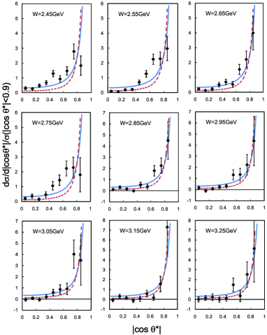
Figure 16: The angular dependence of the differential cross sections in different $W$ regions, with the normalization to the cross section integrated over $|\cos\theta^{*}|<0.9$. The solid and dashed curves are proportional to $1/\sin^{4}\theta^{*}$ and $1/\sin^{6}\theta^{*}$, respectively, normalized similarly.

Figure 16 compares the normalized differential cross sections with the function, $0.322/\sin^{4}\theta^{*}$ (solid curves). The factor in the numerator is calculated by dividing differential cross sections, which are proportional to $1/\sin^{4}\theta^{*}$ by the total integral for $|\cos\theta^{*}|<0.9$. Agreement is poor in the $W$ region considered. A $1/\sin^{6}\theta^{*}$ dependence (dashed curves in the same figure) agrees better with the data for $W>3.0$ GeV. The $\chi^{2}$’s for the $1/\sin^{4}\theta^{*}$ ($1/\sin^{6}\theta^{*}$) dependences are 29.6 (14.3) for the $W=3.05$ GeV bin, 27.8 (7.8) for the $W=3.15$ GeV bin, and 9.8 (4.7) for the $W=3.25$ GeV bin. The number of degrees of freedom is 8, and only statistical errors are used to evaluate the $\chi^{2}$.

A $1/\sin^{4}\theta^{*}$ dependence is not a prediction of perturbative QCD (pQCD) for neutral-meson pair production, and thus the disagreement does not imply an inconsistency with the pQCD model bl . However, it might indicate that the $\eta\eta$ production mechanism is different from that of $\pi^{0}\pi^{0}$ and other production processes where a $1/\sin^{4}\theta^{*}$ dependence describes data well for $W>3.1$ GeV. The handbag model also predicts a $1/\sin^{4}\theta^{*}$ dependence for neutral meson pair production processes at large Mandelstam variable $t$ handbag ; handbag2 . These predictions are critically discussed in Ref. newvlc .

VI.2 $W^{-n}$ dependence

We fit the $W^{-n}$ dependence of the total cross section ($|\cos\theta^{*}|<0.8$, where we take the upper boundary 0.8, to match that in our $\pi^{0}\pi^{0}$ analysis) in the energy region 2.4–3.3 GeV. The fit gives

$$n=7.8\pm 0.6(stat)\pm 0.4(sys),$$ (17)

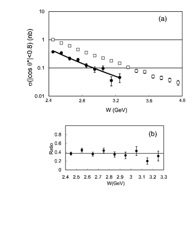
Figure 17: (a) The $W$ dependence of the cross sections ($|\cos\theta^{*}|<0.8$) for the $\pi^{0}\pi^{0}$ (open squares) pi0pi02 and $\eta\eta$ (closed circles) processes. The curve is the power-law fit for the latter process. (b) The $W$ dependence of the cross section ratio of $\eta\eta$ to $\pi^{0}\pi^{0}$ ($|\cos\theta^{*}|<0.8$). The line is the average in the 2.4 - 3.3 GeV range. The error bars are only statistical in the above figures.

and the corresponding cross section is shown in Fig. 17(a) together with that of the $\pi^{0}\pi^{0}$ process in the same angular range.

The systematic error is obtained by simultaneously varying the cross section by $\pm 1\sigma$ at 2.45 GeV and $\mp 1\sigma$ at 3.25 GeV, and by $\mp(W~{}{\rm[GeV]}-2.85)\sigma/0.4$ for the other $W$ points in between, where $\sigma$, amounting to 6%, is the systematic error that does not include the uncertainty in the energy-independent normalization.

The slope parameter, $n$, can be compared with $n$ values in other processes that we have studied earlier nkzw ; wtchen ; pi0pi02 ; etapi0 . The results are summarized in Table 11. The present value for the $\eta\eta$ process is close to that for the $\pi^{0}\pi^{0}$ process, although we note the measured $W$ regions are different. Differences in this parameter among different processes are discussed in Ref. newvlc .

Table 11: The value of $n$ in $\sigma_{\rm tot}\propto W^{-n}$ in various reactions fitted in the $W$ and $|\cos\theta^{*}|$ ranges indicated. The first and second errors are statistical and systematic, respectively.

Process	$n$	$W$ range (GeV)	$|\cos\theta^{*}|$ range	Reference
$\eta\eta$	$7.8\pm 0.6\pm 0.4$	2.4 – 3.3	$<0.8$	This work
$\eta\pi^{0}$	$10.5\pm 1.2\pm 0.5$	3.1 – 4.1	$<0.8$	etapi0
$\pi^{0}\pi^{0}$	$8.0\pm 0.5\pm 0.4$	3.1 – 4.1 (3.3 – 3.6 excluded)	$<0.8$	pi0pi02
$K^{0}_{S}K^{0}_{S}$	$10.5\pm 0.6\pm 0.5$	2.4 – 4.0 (3.3 – 3.6 excluded)	$<0.6$	wtchen
$\pi^{+}\pi^{-}$	$7.9\pm 0.4\pm 1.5$	3.0 – 4.1	$<0.6$	nkzw
$K^{+}K^{-}$	$7.3\pm 0.3\pm 1.5$	3.0 – 4.1	$<0.6$	nkzw

VI.3 Cross section ratio

The ratio of cross sections between neutral-pseudoscalar-meson ($\pi^{0}$ or $\eta$) pairs in two-photon collisions can be predicted relatively reliably in both pQCD and handbag models, based on quark charges and flavor-SU(3) symmetry. The pQCD model bl predictions for the cross section ratios for $\pi^{0}\pi^{0}$, $\eta\pi^{0}$ and $\eta\eta$ are summarized in Table 12. In the table, $R_{f}=(f_{\eta}/f_{\pi^{0}})^{2}$, where $f_{\eta}$ ($f_{\pi}$) is the $\eta$ ($\pi^{0}$) form factor. The value of $R_{f}$ is not well known, and we provisionally assume it to be unity. The ratio of the cross sections is proportional to the square of the coherent sum of the product of the quark charges, $|\Sigma e_{1}e_{2}|^{2}$, in which $e_{1}=-e_{2}$ in the present neutral-meson production cases. We show two predictions: a pure flavor-SU(3) octet state and a mixture with $\theta_{P}=-18^{\circ}$ for the $\eta$ and $\eta^{\prime}$ mesons. Here, we assume that the quark-antiquark component of the neutral meson wave functions dominates and is much larger than the two-gluon component, in obtaining the relations between the cross sections.

The $W$ dependence of the ratio between the measured cross section integrated over $|\cos\theta^{*}|<0.8$ of $\gamma\gamma\to\eta\eta$ to $\gamma\gamma\to\pi^{0}\pi^{0}$ is plotted in Fig. 17(b). For the $\pi^{0}\pi^{0}$ process, the contributions from charmonium production are subtracted using a model-dependent assumption described in Ref. pi0pi02 . We use the $\eta\eta$ result only below $W<3.3$ GeV, where the charmonium contribution is negligibly small. Even though the ratio may have a slight $W$ dependence, in order to compare with QCD (as was done for other processes) we average the ratio of the cross sections over the range $2.4~{}{\rm GeV}<W<3.3~{}{\rm GeV}$ and obtain

$$\frac{\sigma(\eta\eta)}{\sigma(\pi^{0}\pi^{0})}=0.37\pm 0.02(stat)\pm 0.03(sys)$$ (18)

for $|\cos\theta^{*}|<0.8$. The prediction of this model with $\theta_{P}=-18^{\circ}$ and $R_{f}=1$ agrees well with our previous $\eta\pi^{0}$ measurement etapi0 , but it is in poor agreement for the $\eta\eta$ process. However, we note that the $W$ regions are different in the two cases.

The prediction of the $\eta\eta$ cross section for $|\cos\theta^{*}|<0.6$ from the handbag model is presented in Fig. 5 in Ref. handbag2 , which is based on measurements of other meson-pair production processes. We show the results from this measurement, which can be directly compared with the prediction in Table 13. Agreement between the measurement and prediction is fairly good.

Table 12: Predictions and data for the cross section ratios bl for $\pi^{0}\pi^{0}$, $\eta\pi^{0}$ and $\eta\eta$ production processes in two-photon collisions. Here, $R_{f}=(f_{\eta}/f_{\pi^{0}})^{2}$, where $f_{\eta}$ ($f_{\pi}$) is the $\eta$ ($\pi^{0}$) form factor; the value may be taken to be $R_{f}=1$. The $\eta$ meson is treated as a pure SU(3) octet state for the entries in the “octet” row, while “$\theta_{P}=-18^{\circ}$” is the most probable mixing angle between the octet and singlet states from experiment PDG . The first and second errors for the data are statistical and systematic, respectively.

$\eta$ in SU(3)	$\sigma(\eta\pi^{0})/\sigma(\pi^{0}\pi^{0})$	$\sigma(\eta\eta)/\sigma(\pi^{0}\pi^{0})$
Octet	$0.24R_{f}$	$0.36R_{f}^{2}$
$\theta_{P}=-18^{\circ}$	$0.46R_{f}$	$0.62R_{f}^{2}$
Data (ref.)	$0.48\pm 0.05\pm 0.04$ etapi0	$0.37\pm 0.02\pm 0.03$ (this work)
($W$ range)	$(3.1~{}{\rm GeV}<W<4.0~{}{\rm GeV})$	$(2.4~{}{\rm GeV}<W<3.3~{}{\rm GeV})$

Table 13: Cross section integrated over $|\cos\theta^{*}|<0.6$ multiplied by $s^{3}$. The first and second errors are statistical and systematic, respectively.

$s$ (GeV2)	$s^{3}\sigma(|\cos\theta^{*}|<0.6)$ (nb GeV6)
6.00	$38.7\pm 3.7\pm 4.3$
6.50	$33.5\pm 4.1\pm 3.6$
7.02	$28.4\pm 4.5\pm 3.1$
7.56	$38.1\pm 5.6\pm 4.3$
8.12	$17.1\pm 4.3\pm 2.1$
8.70	$21.7\pm 5.9\pm 2.6$
9.30	$18.5\pm 6.4\pm 2.4$
9.92	$11.7\pm 6.8\pm 2.0$
10.56	$21.2\pm 10.6\pm 3.5$

VI.4 Extraction of $\chi_{cJ}$ charmonium contribution

As in our previous $\pi^{0}\pi^{0}$ analysis pi0pi02 , we extract the contributions from the $\chi_{c0}$ and $\chi_{c2}$ charmonia from the $\eta\eta$ data, using the raw yield distribution in the region 2.8 GeV $<W<3.8$ GeV integrated over $|\cos\theta^{*}|<0.4$ (Fig. 18), where the contribution is enhanced against the forward peak from the QCD effect.

The same formula as in our analysis for the $\pi^{0}\pi^{0}$ final state pi0pi02 is used, where partial interference between the $\chi_{c0}$ charmonium and the continuum component is taken into account:

$$Y {}(W)=$$

$$|\sqrt{\alpha kW^{-\beta}}+e^{i\phi}\sqrt{N_{\chi_{c0}}}{\rm BW}_{\chi_{c0}}(W)|^{2}$$

$$+N_{\chi_{c2}}|{\rm BW}_{\chi_{c2}}(W)|^{2}+\alpha(1-k)W^{-\beta},$$

where ${\rm BW}_{\chi_{cJ}}(W)$ is a Breit-Wigner function for the charmonium amplitude, which is proportional to $\sim 1/(W^{2}-M_{\chi_{cJ}}^{2}-iM_{\chi_{cJ}}\Gamma_{\chi_{cJ}})$ and is normalized as $\int|{\rm BW}_{\chi_{cJ}}(W)|^{2}dW=1$. The masses and widths, $M$ and $\Gamma$, of the charmonium states are fixed to the PDG world averages PDG . The component $\alpha W^{-\beta}$ corresponds to the contribution from the continuum, with a fraction $k$ that interferes with the $\chi_{c0}$ amplitude with a relative phase angle, $\phi$.

We do fits with and without interference between the $\chi_{c0}$ and the continuum. The interference with the $\chi_{c2}$ is neglected because of its narrow width. We assume a $W$ resolution to be $0.01W$ from the MC simulation, and take it into account in the fit by smearing the function $Y(W)$. We apply a binned maximum likelihood fit with a bin width $\Delta W=20$ MeV.

The result with interference gives nearly the same result as the fit without interference but with larger errors. The fit with interference cannot determine the interference parameters, $k$ and $\phi$, with a useful accuracy. Therefore, we take the nominal result from the fit without interference. The best fit is shown in Fig. 18. The results are tabulated in Table 14. Significances for the charmonium signals are 5.2$\sigma$ for the $\chi_{c0}$ and 3.0$\sigma$ for the $\chi_{c2}$. The significances are obtained from the difference of the logarithmic-likelihoods with and without the corresponding charmonium contribution, where the change in the number of degrees-of-freedom is taken into account. Here, in order to obtain the most conservative value, we extracted the value in the interference (non-interference) case for the $\chi_{c0}$ ($\chi_{c2}$). The systematic errors are from uncertainties in the $W$ scale and the $W$ resolution (we vary them by $\pm 3$ MeV and by $\pm 20\%$, respectively) and the efficiency error.

The results for $\Gamma_{\gamma\gamma}(\chi_{cJ}){\cal B}(\chi_{cJ}\to\eta\eta)$ are consistent with the product of the known total widths PDG and the branching fractions from the recent CLEO and BES measurements cleobr ; besbr , $(8.0\pm 0.9)$ eV and $(0.30\pm 0.04)$ eV for $\chi_{c0}$ and $\chi_{c2}$, respectively, where we take the average of the CLEO and BES measurements.

Table 14: Charmonium yields and $\Gamma_{\gamma\gamma}{\cal B}(\eta\eta)$ from the present measurement. Two cases are shown: with and without interference between $\chi_{c0}$ and continuum. The first and second (if given) errors are statistical and systematic, respectively. Only differences in log-likelihood values are meaningful.

Interference	Yield($\chi_{c0}$)	Yield($\chi_{c2}$)	$-2\ln L/ndf$	$\Gamma_{\gamma\gamma}(\chi_{c0}){\cal B}(\chi_{c0}\to\eta\eta)$  (eV)	$\Gamma_{\gamma\gamma}(\chi_{c2}){\cal B}(\chi_{c2}\to\eta\eta)$
Without	$21.7\pm 5.3$	$8.5\pm 3.6$	39.5/46	$9.4\pm 2.3\pm 1.2$	$0.53\pm 0.22\pm 0.09$
With	$21.5\pm 9.2$	$10.1\pm 3.9$	38.5/44

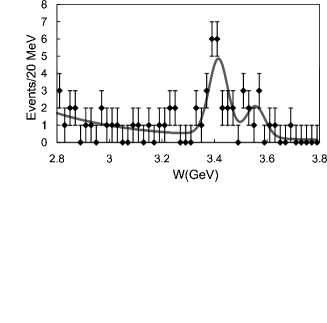
Figure 18: The $W$ distribution in the charmonium region ($|\cos\theta^{*}|<0.4$). The fit does not take interference into account.

VII Summary and Conclusion

We have measured the cross section of $\gamma\gamma\to\eta\eta$ using a high-statistics data sample from $e^{+}e^{-}$ collisions corresponding to an integrated luminosity of 393 fb^-1 with the Belle detector at the KEKB accelerator. We obtain results for the differential cross sections in the center-of-mass energy ($W$) and polar angle ( $|\cos\theta^{*}|$) ranges of 1.096 GeV (the mass threshold) $<W<3.8~{}{\rm GeV}$ and up to $|\cos\theta^{*}|=0.9$ or 1.0, depending on $W$.

The differential cross sections are fitted in the energy regions, 1.12 GeV$<W<$ 1.64 GeV and 1.20 GeV$<W<$ 2.00 GeV using a simple parameterization of the S, D₀ and D₂ waves, assuming that amplitudes consist of resonances and a smooth background. In the low energy fit, consistency of the parameters of the $f_{2}(1270)$ and $f_{2}^{\prime}(1525)$ with previous measurements is checked. The apparent threshold enhancement in the S wave is fitted in terms of a scalar meson, $f_{0}(Y)$, whose mass, width and $\Gamma_{\gamma\gamma}{\cal B}(\eta\eta)$ are obtained to be $1262~{}^{+51}_{-78}~{}^{+82}_{-103}~{}{\rm MeV}/c^{2}$, $484~{}^{+246}_{-170}~{}^{+246}_{-263}~{}{\rm MeV}$ and $121~{}^{+133}_{-53}~{}^{+169}_{-106}~{}{\rm eV}$, respectively. The $f_{0}(Y)$ is introduced only to parameterize the data and may not be a single resonance.

For the energy region of $1.20~{}{\rm GeV}<W<2.00~{}{\rm GeV}$, fits are then performed by fixing most of the parameters obtained in the low energy region and by including an additional tensor resonance. The obtained mass, width and $\Gamma_{\gamma\gamma}{\cal B}(\eta\eta)$ for the tensor meson are $1737~{}\pm 9~{}^{+198}_{-65}~{}{\rm MeV}/c^{2}$, $228~{}^{+21}_{-20}~{}^{+234}_{-153}~{}{\rm MeV}$ and $5.2~{}^{+0.9}_{-0.8}~{}^{+37.3}_{-4.5}$ eV, respectively. The $f_{2}(X)$ is a parameterization used to describe the data in 1700 MeV mass region. It may represent some of the possible tensor resonances in this mass region.

We observe clear signals from $f_{2}(1270)\to\eta\eta$ and $f^{\prime}_{2}(1525)\to\eta\eta$ for the first time in two-photon collisions. The product $\Gamma_{\gamma\gamma}{\cal B}(\eta\eta)$ for the $f_{2}(1270)$ is $11.5~{}^{+1.8}_{-2.0}~{}^{+4.5}_{-3.7}$ eV. Our $f_{2}(X)$ may correspond to the $f_{2}(1810)$ state reported in Ref. kmat . The result of our measurements for the product $\Gamma_{\gamma\gamma}{\cal B}(\eta\eta)$ for the $f_{2}(1270)$ and $f^{\prime}_{2}(1525)$ are consistent with the previously known values PDG ; gams ; wa102 ; gams2 ; kmat .

The angular dependence of the differential cross section in the 2.4–3.3 GeV region are compared with $\sim 1/\sin^{4}\theta^{*}$ dependence, as found in the $\pi^{0}\pi^{0}$ process pi0pi02 and predicted by the handbag model handbag ; handbag2 for $W>3.1$ GeV. However, in the $\eta\eta$ process, a $1/\sin^{4}\theta^{*}$ dependence is not found in the data for the the energy region where the measurement is performed.

The slope parameter $n$ for the cross section, $\sigma(W)\sim W^{-n}$, in a similar $W$ region is close to that measured in the $\pi^{0}\pi^{0}$ process pi0pi02 .

The measured cross section ratio, $\sigma(\eta\eta)/\sigma(\pi^{0}\pi^{0})=0.37\pm 0.02\pm 0.03$ (for $|\cos\theta^{*}|<0.8$), is compared with the prediction of pQCD bl with a pseudoscalar meson mixing angle, $\theta_{P}=-18^{\circ}$. We find that the assumption for the squared form-factor ratio, $R_{f}=(f_{\eta}/f_{\pi^{0}})^{2}=1$, which is in a good agreement with the ratio $\sigma(\eta\pi^{0})/\sigma(\pi^{0}\pi^{0})$ etapi0 cannot reproduce well the $\eta\eta$ measurement. Our result agrees rather well with the recent handbag model prediction handbag2 .

Charmonium contributions in the $\eta\eta$ process are confirmed for the first time. Our measurements are consistent with the known partial decay widths of the $\chi_{c0}$ and $\chi_{c2}$ to $\gamma\gamma$ PDG and $\eta\eta$ cleobr ; besbr final states.

References

- (1) T. Mori et al. (Belle Collaboration), Phys. Rev. D 75, 051101(R) (2007).
- (2) T. Mori et al. (Belle Collaboration), J. Phys. Soc. Jpn 76, 074102 (2007).
- (3) H. Nakazawa et al. (Belle Collaboration), Phys. Lett. B 615, 39 (2005).
- (4) K. Abe et al. (Belle Collaboration), Eur. Phys. J. C 32, 323 (2004).
- (5) W.T. Chen et al. (Belle Collaboration), Phys. Lett. B 651, 15 (2007).
- (6) C.C. Kuo et al. (Belle Collaboration), Phys. Lett. B 621, 41 (2005).
- (7) S. Uehara et al. (Belle Collaboration), Phys. Rev. Lett. 96, 082003 (2006).
- (8) S. Uehara et al. (Belle Collaboration), Phys. Rev. Lett. 104, 092001 (2010).
- (9) C.P. Shen et al. (Belle Collaboration), Phys. Rev. Lett. 104, 112004 (2010).
- (10) S. Uehara, Y. Watanabe et al. (Belle Collaboration), Phys. Rev. D 78, 052004 (2008).
- (11) S. Uehara, Y. Watanabe, H. Nakazawa et al. (Belle Collaboration), Phys. Rev. D 79, 052009 (2009).
- (12) S. Uehara, Y. Watanabe, H. Nakazawa et al. (Belle Collaboration), Phys. Rev. D 80, 032001 (2009).
-
(13)
See, e.g., the compilation in
http://durpdg.dur.ac.uk/spires/hepdata/
online/2gamma/2gammahome.html. - (14) S.J. Brodsky and G.P. Lepage, Phys. Rev. D 24, 1808 (1981).
- (15) M. Diehl, P. Kroll and C. Vogt, Phys. Lett. B 532, 99 (2002).
- (16) M. Diehl and P. Kroll, Phys. Lett. B 683, 165 (2010).
- (17) A. Abashian et al. (Belle Collaboration), Nucl. Instr. and Meth. A 479, 117 (2002).
- (18) S. Kurokawa and E. Kikutani, Nucl. Instr. and Meth. A 499, 1 (2003), and other papers included in this volume.
- (19) S. Uehara, KEK Report 96-11 (1996).
- (20) Particle Data Group, C. Amsler et al., Phys. Lett. B 667, 1 (2008) and 2009 partial update for the 2010 edition.
- (21) F. Binon et al., Phys. Atom. Nucl. 68, 960 (2005) (Translated from Yad. Fiz., 68, 998 (2005)).
- (22) D. Barberis et al. (WA102 Collaboration), Phys. Lett. B 479, 59 (2000).
- (23) F. Binon et al. Phys. Atom. Nucl. 70, 1713 (2007) (Translated from Yad. Fiz., 70, 1758 (2007)).
- (24) R. S. Longacre et al., Phys. Lett. B 177, 223 (1986).
- (25) J.M. Blatt and V.F. Weisskopf, Theoretical Nuclear Physics (Wiley, New York, 1952), pp. 359-365 and 386-389.
- (26) G. Grayer et al., Nucl. Phys. B 75, 189 (1974); A. Garmash et al. (Belle Collaboration), Phys. Rev. D 71, 092003 (2005); B. Aubert et al. (BaBar Collaboration), Phys. Rev. D 72, 052002 (2005).
- (27) V. L. Chernyak, arXiv:0912.0623[hep-ph] (2009).
- (28) D. M. Asner et al. (CLEO Collaboration), Phys. Rev. D 79, 072007 (2009).
- (29) M. Ablikim et al. (BES Collaboration), Phys. Rev. D 81, 052005 (2010).