Rotating thin-disk galaxies through the eyes of Newton

Abstract

By numerically solving the mass distribution in a rotating disk based on Newton’s laws of motion and gravitation, we demonstrate that the observed flat rotation curves for most spiral galaxies correspond to exponentially decreasing mass density from galactic center for the most of the part except within the central core and near periphery edge. Hence, we believe the galaxies described with our model are consistent with that seen through the eyes of Newton. Although Newton’s laws and Kepler’s laws seem to yield the same results when they are applied to the planets in the solar system, they are shown to lead to quite different results when describing the stellar dynamics in disk galaxies. This is because that Keplerian dynamics may be equivalent to Newtonian dynamics for only special circumstances, but not generally for all the cases. Thus, the conclusions drawn from calculations based on Keplerian dynamics are often likely to be erroneous when used to describe rotating disk galaxies.

PACS numbers: 95.75.Pq, 98.35.Ce, 98.35.Df

1 Introduction

A galaxy is a stellar system consisting of a massive gravitationally bound assembly of stars, an interstellar medium of gas and cosmic dust, etc. Observations have shown that many (mature spiral) galaxies share a common structure with the visible matter distributed in a flat thin disk (as in figure 1), rotating about their center of mass in nearly circular orbits [1]. Apparently, this typical behavior of galaxies is similar to that of our solar system with planets orbiting around the Sun in a flat planetary plane.

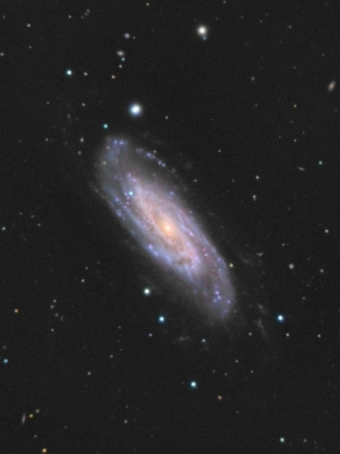
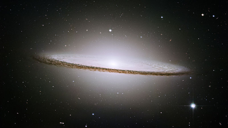
Figure 1: Spiral galaxies: NGC 3198 and NGC 4594–also known as M 104 sombrero galaxy.

For planets orbiting around the Sun, Kepler’s laws of planetary motion (obtained empirically) can provide accurate description. Yet it was Isaac Newton, in his “Philosophiae Naturalis Principia Mathematica”, who used mathematical expressions to show that Kepler’s laws are consequences of Newton’s laws of motion and universal law of gravitation [2]. In addition, Newton found that Kepler’s laws were only part of the story of how objects move in response to gravity. With his laws being discovered by analyzing the orbits of planets around the Sun, Kepler had no reason to believe that his laws would apply to other cases such as moons orbiting planets or comets orbiting the Sun. But Newton was able to derive more general rules that can explain the motion of objects throughout the universe, by analyzing his equations of gravity and motion. Therefore, Newton’s laws of motion and gravity have become a crucial part of the foundation of modern astronomy, whereas Kepler’s laws can become misleading if not applied correctly with sufficient care to cases other than planets orbiting the Sun. For example, Kepler’s third law, stating that more distant objects rotate around the center at slower average speeds, cannot describe the typically observed flat orbital velocity that remains invariant for most part of a galaxy outside its central core [3, 4, 5, 6].

The fundamental difference between a galaxy and the solar system is that the mass is apparently distributed across the entire galaxy whereas the solar system has its mass concentrated at the center in the Sun. Each planet in the solar system can be quite reasonably treated as a point mass moving in a spherically symmetric gravitational field stemming from a large central point mass. The spherical symmetry of gravitational field in the solar system greatly simplifies the mathematical analysis, because the gravitational potential at any position is basically determined by the distance from the center and the mass of the Sun, with contributions from other planets negligible. Actually, the treatment similar to that for the solar system can be directly extended to the situation of distributed mass system as long as it retains the spherical symmetry, except that now the equivalent mass at the center is not a constant but equals to the mass enclosed by the concentric spherical surface through that point of interest. According to Newton’s first and second theorems, if certain amount of mass is uniformly distributed in a spherical shell, this shell exerts no net (gravitational) force on any mass at any point inside it but attracts any mass outside it as if its mass is concentrated at the center [1]. Unfortunately, the thin-disk galaxies do not possess such a simplification-enabling spherical symmetry. So, much more sophisticated mathematical treatments are needed to correctly apply Newton’s laws to the thin-disk galaxies.

Here in this work, we demonstrate an effective numerical method for computing either mass density distribution for a given orbital velocity profile or vice versa by solving the governing equations based on Newton’s laws for an axisymmetric thin-disk galaxy of finite size. We also quantitatively illustrate the possible misleading results due to incorrect application of Kepler’s laws to the same thin-disk galaxy. In other words, we show that the observed behavior of disk galaxies can be described and explained by application of Newton’s laws, but not by Kepler’s laws that may only be regarded as a special case derived from Newton’s laws for spherically symmetric gravitational field.

2 Governing equations

Because much of the mass of a galaxy resides in stars, we can in principle compute gravitational field of a large collection of stars by adding the point-mass fields of all the stars together for any spot of interest. For convenience of mathematical treatment, however, here we represent a galaxy by a continuum of axisymmetrically distributed mass in a circular disk of radius $R_{g}$ as shown in figure 2. Thus, in the present model we consider continuous mass density distribution instead of discrete mass points scattered throughout the disk. This kind of approximation is typically valid when the mass density in stars is viewed on a scale that is small compare to the size of the galaxy, but large compared to the mean distance between stars [1]. Physically, the stars in a galaxy must rotate about the galactic center to maintain the disk shape. Without the centrifugal effect due to rotation, the stars would collapse into the galactic center as a consequence of the gravitational field. It is also reasonable to assume the galaxy is in an approximately steady state with the gravitational force and centrifugal force balancing each other, in view of the fact that most disk stars have completed a large number of revolutions [1].

Let’s consider the force density on a test mass at $(r,\theta=0)$ generated by the gravitational attraction due to the summation (or integration) of a distribution of mass density $\rho(\hat{r})$ at position described by the variables of integration $(\hat{r},\hat{\theta})$. Here the distance between $(r,\theta)$ and $(\hat{r},\hat{\theta})$ is $(\hat{r}^{2}+r^{2}-2\hat{r}r\cos\hat{\theta})^{1/2}$ and the vector projection between the two points is $(\hat{r}\cos\hat{\theta}-r)$. Thus in a steady state, the mechanical balance between the gravitational force (due to the summation of mass in a series of concentric rings) and centrifugal force at every test point ($r$, $\theta=0$) on the disk, according to Newton’s laws of motion and gravitation, can be written as an integration equation (in terms of force per unit mass)

$$\int_{0}^{1}\left[\int_{0}^{2\pi}\frac{(\hat{r}\cos\hat{\theta}-r)d\hat{\theta}}{(\hat{r}^{2}+r^{2}-2\hat{r}r\cos\hat{\theta})^{3/2}}\right]\rho(\hat{r})h\hat{r}d\hat{r}+A\frac{V(r)^{2}}{r}=0\,,$$ (1)

where all the variables are made dimensionless by measuring lengths (e.g., $r$, $\hat{r}$, $h$) in units of the outermost galactic radius $R_{g}$, disk mass density ($\rho$) in units of $M_{g}/R_{g}^{3}$ with $M_{g}$ denoting the total galactic mass, and velocities [$V(r)$] in units of the characteristic galactic rotational velocity $V_{0}$ (as usually defined according to the problem of interest). The disk thickness $h$ is assumed to be constant and small in comparison with the galactic radius $R_{g}$. The results are expected to be insensitive to the exact value of this ratio as long as it is small. There is no difference in terms of physical meaning between the notations $(r,\theta)$ and $(\hat{r},\hat{\theta})$; but mathematically the former denotes the independent variables in the integral equation (for $\theta=0$) whereas the latter the variables of integration. The gravitational force represented as the summation of a series of concentric rings is described by the first term (double integral) while the centrifugal forces are described by the second term in (1).

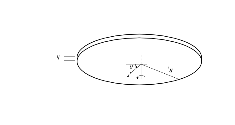
Figure 2: Definition sketch of the thin-disk model considered in the present work. The mass is assumed to distribute axisymmetrically in the circular disk of uniform thickness $h$ with a variable density as a function of radial coordinate $r$ (but independent of the polar angle $\theta$).

Our process of nondimensionalization of the force-balance equation yields a dimensionless parameter, which we call the “galactic rotation number” $A$, as given by

$$A\equiv\frac{V_{0}^{2}\,R_{g}}{M_{g}\,G}\,,$$ (2)

where $G$ ($=6.67\times 10^{-11}$ [m³/(kg s²)]) denotes the gravitational constant, $R_{g}$ is the outermost galactic radius, and $V_{0}$ is the characteristic velocity (which may be equated here to the maximum asymptotic rotational velocity of a disk galaxy). This galactic rotation number $A$ simply displays the ratio of centrifugal forces to gravitational forces. For typical galactic values of $R_{g}$, $V_{0}$, and $M_{g}$ we obtain $A\sim 1.6$ as will be shown in detail later.

When solving for the mass density $\rho(r)$ with $V(r)$ given, we need to impose an overall constraint such that the total mass of the galaxy $M_{g}$ is constant, namely,

$$2\pi\int_{0}^{1}\rho(\hat{r})h\hat{r}d\hat{r}=1.$$ (3)

This constraint due to the conservation of mass can actually be used to determine the value of galatic rotation number $A$.

It is known that the integral with respect to $\hat{\theta}$ in (1) can be written as [1] (pp. 72-73)

$$\int_{0}^{2\pi}\frac{(\hat{r}\cos\hat{\theta}-r)d\hat{\theta}}{(\hat{r}^{2}+r^{2}-2\hat{r}r\cos\hat{\theta})^{3/2}}=2\left[\frac{E(m)}{r(\hat{r}-r)}-\frac{K(m)}{r(\hat{r}+r)}\right]\,,$$ (4)

where $K(m)$ and $E(m)$ denote the complete elliptic integrals of the first kind and second kind, with

$$m\equiv\frac{4\hat{r}r}{(\hat{r}+r)^{2}}\,.$$

Thus, (1) becomes

$$\int_{0}^{1}\left[\frac{E(m)}{\hat{r}-r}-\frac{K(m)}{\hat{r}+r}\right]\rho(\hat{r})h\hat{r}d\hat{r}+\frac{1}{2}AV(r)^{2}=0\,.$$ (5)

Equations (5) and (3) can be used to determine the mass density distribution $\rho(r)$ in the disk, the galactic rotation number $A$, and subsequently the total galactic mass $M_{g}$, all from measured values of $V(r)$, $R_{c}$, $R_{g}$ and $V_{0}$. Seemingly complicated as it might be, these equations for $\rho(r)$ actually constitute a linear mathematical problem that guarantees uniqueness of solutions. Conversely, these equations can also be used to determine the orbital velocity $V(r)$ if the mass density distribution $\rho(r)$ is known. This is a well-defined mathematical problem completely deducible from the available input data.

Because our governing equations are derived according to Newton’s laws, they must be applicable to the solar system. As an example for $\rho(r)=\delta(r)/(\pi\,r)$ (namely, the Dirac delta function in two-dimensional polar coordinates), (1) or (5) would yield

$$-\frac{1}{r}+A\,V(r)^{2}=0\,,$$

which is exactly the familiar formula for so-called Keplerian velocity based on Kepler’s third law of planetary motion

$$V_{0}\,V(r)=\sqrt{\frac{G\,M_{g}}{R_{g}\,r}}\,,$$ (6)

where $V_{0}\,V(r)$ is the dimensional orbital velocity, $M_{g}$ is basically the mass of the Sun, and $R_{g}\,r$ the dimensional distance from the Sun.

For a galaxy with mass distribution that is not spherically symmetric, simple closed-form analytical solutions may not be tractable. Yet accurate numerical solutions can be computed with appropriately implemented computational techniques as detailed in Appendix A. What it amounts to is nothing more than solving a linear algebra matrix problem using a well-established matrix solver.

3 Mass distribution determined from given rotation curve

The measurements of galactic rotational velocity profiles (also known as “rotation curves”) of mature spiral galaxies reveal that the rotation velocity typically rises linearly from the galactic center (as if the local mass were in rigid body rotation) in a relatively small core, and then with the slope decreasing continuously in a narrow transition zone it reaches an approximately constant (flat) velocity extending to the galactic periphery [3, 4, 5, 6]. These essential features may be mathematically idealized as

$$V(r)=1-e^{-r/R_{c}}\,,$$ (7)

where $V(r)$ denotes the (dimensionless) orbital velocity (as measured in units of the maximum velocity in the flat part that may be regarded as the characteristic velocity of galactic rotation $V_{0}$), and $r$ the radial coordinate from the galactic center (in units of the outermost galactic disk radius $R_{g}$). The parameter $R_{c}$ can be used to describe various radii of the ”cores” of different galaxies. Close to the galactic center, namely when $r/R_{c}$ is small, we have $V(r)\sim r/R_{c}$, describing a linearly rising rotation velocity, by virtue of the Taylor expansion of $e^{-r/R_{c}}$. Figure 3 shows typical galactic rotation curves described by (7).

Figure 3: Nondimensionalized orbital velocity profiles $V(r)$ according to the mathematically idealized formula (7) for $R_{c}=0.015$, $0.03$, $0.05$ and $0.1$.

With $V(r)$ given by (7), the mass density distribution $\rho(r)$ and the value of $A$ can be determined by computing solution to (21) and (23). To compute numerical solutions, the value of disk thickness $h$ must be provided; we assume $h=0.01$ (based on the measurements for the Milky Way galaxy). By using $N=1001$ nonuniformly distributed nodes we found the obtained curves of $\rho(r)$ become reasonably smooth and the values of galactic rotation number $A$ are discretization-independent.

Shown in figure 4 are the computed mass density distributions $\rho(r)$ that satisfy the galactic rotation curves in figure 3. It is at the galactic center where mass attains the highest density. Away from the galactic center, the mass density decreases rapidly (with a slope becoming steeper for a tigher galactic core indicated by smaller $R_{c}$). However, beyond $R_{c}$, the mass density decreases rather gradually towards the galactic periphery until reaching the galactic edge where it takes a sharp drop. Noteworthy here is that the computed values of galactic rotation number $A$ are within a small range around $1.6$ despite an order-of-magnitude variation of the galactic core radius $R_{c}$.

Figure 4: The distributions of mass density $\rho(r)$ computed based on Newtonian dynamics and given rotation curves for $R_{c}=0.015$, $0.03$, $0.05$, and $0.1$, with $A=1.5714$, $1.5733$, $1.5777$, and $1.5999$ determined as part of the numerical solutions.

As apparent in figure 4, the computed $\log\rho$ decreases almost linearly with $r$ except for $r<0.1$ (within the central galactic core) and $r>0.9$ (near the galactic edge). This general feature is quite similar to the measured brightness distributions (in typical spiral galaxies) that are commonly fitted in an exponential form with regions of central core and outer edge truncated. For the case of $R_{c}=0.015$ and $A=1.5714$, a least-square fit of our computed $\log\rho$ versus $r$ for $0.1\leq r\leq 0.9$ yields

$$\log\rho=5.4179-3.6802\,r\,.$$ (8)

This actually corresponds to an exponential function $\rho=\rho_{0}\,e^{-r/R_{d}}$ with

$$\rho_{0}=225.4\mbox{ and }R_{d}=0.2717\,,$$ (9)

which is known not to be able to generate the observed flat rotation curves [7, 1]. Thus the much more rapid decrease of $\log\rho$ in the small intervals [0, 0.1) and (0.9, 1] must play important roles in compensating the deficiencies of the simple exponential mass density distribution for matching the commonly observed (flat) rotation curves. If we assume the mass density follows roughly the exponential distribution $\rho=\rho_{0}\,e^{-r/R_{d}}$, we would have the cumulative mass from the galactic center given by

$$2\pi h\int_{0}^{r}\rho_{0}e^{-\hat{r}/R_{d}}\hat{r}d\hat{r}=2\pi h\rho_{0}[R_{d}^{2}-R_{d}(r+R_{d})e^{-r/R_{d}}]\,.$$ (10)

At $r=1$, this yields a value of $0.922$ for $\rho_{0}=225.4$ and $R_{d}=0.2717$, indicating the exponential mass density distribution is likely to describe about $90\%$ of the mass in a disk galaxy. Another $\sim 10\%$ of the galactic mass seems to reside in the galactic core which may not follow the same exponential distribution (cf. figure 4).

From the knowledge of $V_{0}$ and $R_{g}$ from measured rotation curves, we can determine the value of $M_{g}$ based on computed value of the galactic rotation number $A$ (cf. (2)) as

$$M_{g}=\frac{V_{0}^{2}\,R_{g}}{A\,G}\,.$$ (11)

Because our computed $A$ varies little from $1.6$ for various $R_{c}$, (11) suggests a general relationship of $M_{g}\propto V_{0}^{2}R_{g}$ as what Bosma [5] found from evaluating mass versus size in a large number of observed disk galaxies. In view of the fact that the values of $V_{0}$ are typically around $200$ (km/s), we then believe that the disk size of galaxies $R_{g}$ must be finite in order to keep the total mass of a galaxy $M_{g}$ from becoming infinity. Suggesting finite disk size of galaxies does not necessarily mean that the mass density becomes zero outside the disk edge. We believe that the mass density beyond the galactic edge approaches the inter-galactic level of value and is roughly spherically symmetric, which leads to inconsequential gravitational effect on rotation dynamics in the disk part.

If we take the rotation curve with $R_{c}=0.015$ in figure 3 as that of the Milky Way, we have the galactic rotation number $A=1.57$. Then, from measured Milky Way values $V_{0}=2.2\times 10^{5}$ (m/s) and $R_{g}=5\times 10^{4}$ (light-years) $=4.73\times 10^{20}$ (m), (11) yields

$$M_{g}=2.19\times 10^{41}(\mbox{kg})=1.10\times 10^{11}(\mbox{solar-mass})\,.$$ (12)

This value is in very good agreement with the Milky Way star counts of 100 billion [8], further including additional dust, grains, lumps, gases and plasma in all galaxies.

With the given values of $M_{g}$ and $R_{g}$, we can estimate the computed ‘radial scale’ $R_{d}\,R_{g}=4.0$ (kpc) $=1.234\times 10^{20}$ (m) and the exponential disk central (surface) mass density $\rho_{0}hM_{g}/R_{g}^{2}=1340$ (solar-mass / pc²) based on (8) for the Milky Way galaxy. (Here, $1$ (pc) $=3.086\times 10^{16}$ (m) and $1$ (solar mass) $=1.99\times 10^{30}$ (kg).) Compared with the results from fitting the brightness measurement data, e.g., the radial scale of $2.5$ (kpc) and exponential disk central brightness of $867$ (solar-luminosity / pc²) [9], our computational results indicate either generally dimmer stars (than the Sun) or considerable amounts of cold gas exist throughout the Milky Way with the total mass density decreasing at slower rate than that of the brightness (i.e., luminosity density).

Another example is the galaxy NGC 3198, which has a (nearly idealized, often cited) rotation curve with $V_{0}=1.5\times 10^{5}$ (m/s), $R_{g}=30$ (kpc) $=9.24\times 10^{20}$ (m), and $R_{c}\sim 0.015$. Again with $A=1.57$, we obtain $M_{g}=1.98\times 10^{41}$ (kg) $=9.9\times 10^{10}$ (solar-mass). As with the Milky Way, we can also predict the radial scale and exponential central mass density for NGC 3198 as $8.16$ (kpc) and $250$ (solar-mass / pc²), respectively (based on $\rho_{0}=225.4$ and $R_{d}=0.2717$ from (8). Compared with the radial luminosity profile (which suggested an exponential disk with a radial scale of $2.63$ (kpc) and central brightness $212$ (solar-luminosity / pc²) based on a total luminosity of $9.0\times 10^{9}$ (solar-luminosity) [10], our predicted mass density appears to decrease much more slowly with stars (or mass objects) generally dimmer than the Sun.

Hence, the results computed here, as if they were obtained by Newton applying his laws of motion and gravitation to solve the governing equations (1) and (3), seem to be reasonably consistent with the observational measurements. In other words, the rotating thin-disk galaxies through the eyes of Newton are nothing more than massive gravitationally bound assemblies of objects governed by his same laws for the planet’s motion in the solar system albeit more sophiscated mathematical treatments are needed to obtain the correct description than those with the planets in the solar system.

4 Results based on Keplerian dynamics

In the literature, many authors [2, 8, 11, 12, 13, 14] tend to simply apply Keplerian dynamics (which was derived from gravitational field generated by a spherically symmetric distribution of mass) when analyzing the rotation behavior of thin-disk galaxies. For example, Volders [11] demonstrated that spiral galaxy M33 does not spin as expected according to Keplerian dynamics–a result which was later extended to many other spiral galaxies [3, 4, 5, 6].

Strictly speaking, a Keplerian potential (due to a point mass $M$ as that for the solar system) is expressed as

$$\Phi(r)=-\frac{G\,M}{r}\,,$$ (13)

For a distributed mass with spherical symmetry, the generalized form of Keplerian potential becomes

$$\Phi(r)=-\frac{G\,M(r)}{r}\,,$$ (14)

where $M(r)$ denotes the amount of mass enclosed by the concentric spherical surface of radius $r$ [1]. Although (14) comes from the assumption of spherical symmetry, it has often been used to determine the mass distribution and the total mass of a (disk) galaxy from a measured rotation curve, with $M(r)$ denoting the mass interior to radius $r$ from the galactic center. For example, in the recent versions of textbooks by Bennett et al. [2], Sparke and Gallagher [8], and Keel [12], the value of $M(r)$ (also denoted as $M_{r}$ or $M(<r)$) in a disk galaxy is simply determined from a known rotation curve $V(r)$ by

$$M(r)=\frac{r\,V(r)^{2}}{G}\,,$$ (15)

which has basically the same mathematical form as (6).

According to (15), we would have an equation based on Keplerian dynamics for force balance as

$$2\pi\,h\int_{0}^{r}\rho(\hat{r})\hat{r}d\hat{r}-A\,r\,V(r)^{2}=0\,,$$ (16)

instead of (1). Here, the difference in mathematical forms between (16) and (1) should be quite clear. But whether there are much of practical differences between the two may not be obvious. For example, authors like Sparke and Gallagher [8] and Keel [12] attempted to justify their usages of Keplerian formula for rotating thin disk galaxies by stating that the result due to Keplerian formula does not differ more than $20\%$ from the actual result, without showing a quantitative comparison. Therefore, we would like to examine a few comparative examples to see whether Keplerian dynamics (16) can be practically used as a close approximation to Newtonian dynamics (1) for disk galaxies.

For the orbital velocity $V(r)$ given by (7), an analytical solution to (16) for $\rho(r)$ can be obtained as

$$\rho(r)=\frac{A}{2\pi\,h}\left[\frac{1}{r}\left(1-2e^{-r/R_{c}}+e^{-2r/R_{c}}\right)+\frac{2}{R_{c}}\left(e^{-r/R_{c}}-e^{-2r/R_{c}}\right)\right]\,.$$ (17)

It is not difficult to prove that $\rho(r)\to 0$ as $r\to 0$, as in sharp contrast to that obtained according to Newton’s laws shown in figure 4. For $r>>R_{c}$ (i.e., outside the galactic core), (17 describes $\rho(r)\propto 1/r$, as expected for the part where $V(r)$ is flat (constant) such that the first term in (16) becomes proportional to $r$. In fact, many astronomers often consider the flat rotation curves, i.e., $V(r)=constant$, to indicate that the mass of a disk galaxy should continue to increase linearly well beyond its bright central region because $r\,V(r)^{2}\propto r$ [13, 14].

To satisfy (3), the value of $A$ in (17) is given by

$$A=\frac{1}{1-2e^{-1/R_{c}}+e^{-2/R_{c}}}\,.$$ (18)

When $R_{c}$ is small, e.g., $R_{c}=0.015$, we have $e^{-1/R_{c}}\to 0$, e.g., $e^{-1/0.015}\sim 10^{-29}$; therefore, $A\approx 1$ according to (18). This is in sharp contrast to the result based on formulas for disk galaxies (which predicts $A=1.57$). If $A=1$ were used in (11), we would have the total mass in Milky Way equal to $2.2\times 10^{11}$ (solar-mass)–much more than that given by (12) and the Milky Way star counts.

As a comparison, the distribution of $\rho(r)$ shown in figure 4 for $R_{c}=0.015$ and that given by (17) with $A=1$ are shown in figure 5. Now, the differences between the two are obvious: the Keplerian mass density behaves totally differently in the galactic core with $\rho(r)\to 0$ whereas that numerically obtained in § 3 has $\rho(r)$ monotonically decreasing with $r$ from its maximum value at galactic center to periphery. Outside the galactic core, the Keplerian mass density shows much slower decay ($\propto 1/r$) toward the galactic periphery whereas that obtained numerically in § 3 seems to be approximately exponential. Therefore, the mass density distribution determined based on Keplerian dynamics (16) cannot be a good approximation to the actual $\rho(r)$ obtained numerically in § 3 with Newton’s laws strictly applied.

Figure 5: The distribution of mass density $\rho(r)$ computed based on Newtonian dynamics for $R_{c}=0.015$ (solid) and that derived based on Keplerian dynamics given by (17) with $A=1$ and $R_{c}=0.015$ (dotted).

On the other hand, if the mass density $\rho(r)$ is known as obtained in § 3 for the case of $R_{c}=0.015$ with $A=1.5714$, we can compute the corresponding $V(r)$ from (16). figure 6 shows that the $V(r)$ from (16) clearly differs from that of (7), with rotation velocity decreasing with the radial distance $r$ toward the galactic periphery as expected from Kepler’s third law. Again, this suggests that (16) according to the Keplerian dynamics cannot be a good approximation to the actual galactic dynamics.

Figure 6: The rotation curve of $R_{c}=0.015$ described by (7) (solid) from Newtonian dynamics and that determined from (16) based on the Keplerian dynamics with the known $\rho(r)$ for $R_{c}=0.015$ obtained in § 3 with $A=1.5714$ (dotted).

As demonstrated in § 3, we believe that Newton’s laws of motion and gravitation can adequately describe the dynamical behavior of (disk) galaxies, with appropriate mathematical treatments. Kepler’s laws should not be regarded as the same as Newton’s laws. Newton’s laws can explain Kepler’s laws for the planets in the solar system; but Kepler’s laws cannot be extended to the galactic dynamics like Newton’s laws, even in an approximation sense as shown in figure 5 and figure 6.

5 Conclusions

By strictly applying Newton’s laws, the present computational model can yield mass distributions from the observed galactic rotation curves, as apparently quite consistent with the observed near exponential brightness distributions. Thus through the eyes of Newton, galaxies are nothing more than graviationally bound assemblies of massive objects that are governed by his same laws for the planet’s motion in the solar system. Although Newton’s laws and Kepler’s laws seem to yield the same results when they are applied to the planets in the solar system, they can lead to quite different results when describing the stellar dynamics in disk galaxies (cf. figure 5 and figure 6). If not careful, simply extending Kepler’s laws to the disk galaxies with subtensively distributed mass can suggest misleading conclusions.

As demonstrated in § 4, substituting the computed mass density distribution $\rho(r)$ based on Newtonian dynamics into the Keplerian force-balance equation (16) would yield a rotation curve with orbital velocity decreasing toward galactic periphery (see figure 6). This had led many authors to believe that the visible mass in a galaxy cannot explain the observed flat rotation curve [13, 14, 15]. Therefore, some authors have speculated that some kind of invisible matter called dark matter must exist in the galaxy [2, 13, 14, 15]. Other authors believed modification of Newton’s laws to be needed [16]. The fundamental problem here is that astronomers tend to determine the ‘visible’ mass in a galaxy from the measured brightness based on an over-simplified mass-to-light ratio [15]. When the mass distribution so estimated did not generate the observed flat rotation curve, especially when the Keplerian dynamics was used for another over-simplification, it is often referred to as the ‘galactic rotation problem’ suggesting that there is a discrepancy between the observed rotation speed of matter in the disk and the predictions of Newtonian dynamics [2, 13, 14, 15, 16]. But we believe that Newtonian dynamics can adequately explain the stellar dynamics in disk galaxies when applied correctly; neither the introduction of dark matter nor modification of Newtonian dynamics is needed for explaining the observed rotation curve [17, 18]. Hence, the rotating disk galaxies described with our model must be that seen through the eyes of Newton.

Appendix A Computational techniques

Following a standard boundary element method [19, 20], the governing equations (5) and (3) can be discretized by dividing the one-dimensional problem domain $[0,1]$ into a finite number of line segments called (linear) elements. Each element covers a subdomain confined by two end nodes, e.g., element $n$ corresponds to the subdomain $[r_{n},r_{n+1}]$, where $r_{n}$ and $r_{n+1}$ are nodal values of $r$ at nodes $n$ and $n+1$, respectively. On each element, which is mapped onto a unit line segment $[0,1]$ in the $\xi$-domain (i.e., the computational domain), $\rho$ is expressed in terms of the linear basis functions as

$$\rho(\xi)=\rho_{n}(1-\xi)+\rho_{n+1}\xi\,,\quad 0\leq\xi\leq 1\,,$$ (19)

where $\rho_{n}$ and $\rho_{n+1}$ are nodal values of $\rho$ at nodes $n$ and $n+1$, respectively. Similarly, the radial coordinate $r$ (as well as $\hat{r}$) on each element is also expressed in terms of the linear basis functions by so-called isoparameteric mapping:

$$r(\xi)=r_{n}(1-\xi)+r_{n+1}\xi\,,\quad 0\leq\xi\leq 1\,.$$ (20)

If $V(r)$ is given (e.g., from measurements), the $N$ nodal values of $\rho_{n}=\rho(r_{n})$ can be determined by solving $N$ independent residual equations over $N-1$ element obtained from the collocation procedure, i.e.,

$$\sum_{n=1}^{N-1}\int_{0}^{1}\left[\frac{E(m_{i})}{\hat{r}(\xi)-r_{i}}-\frac{K(m_{i})}{\hat{r}(\xi)+r_{i}}\right]\rho(\xi)h\hat{r}(\xi)\frac{d\hat{r}}{d\xi}d\xi+\frac{1}{2}AV(r_{i})^{2}=0\,,\,i=1,2,...,N\,,$$ (21)

with

$$m_{i}(\xi)\equiv\frac{4\hat{r}(\xi)r_{i}}{[\hat{r}(\xi)+r_{i}]^{2}}\,,$$ (22)

where $\rho(\xi)=\rho_{n}(1-\xi)+\rho_{n+1}\xi$ and $\hat{r}(\xi)=\hat{r}_{n}(1-\xi)+\hat{r}_{n+1}\xi$. The value of $A$ can also be solved by the addition of the constraint equation

$$2\pi\sum_{n=1}^{N-1}\int_{0}^{1}\rho(\xi)h\hat{r}(\xi)\frac{d\hat{r}}{d\xi}d\xi-1=0\,.$$ (23)

Thus, we have $N+1$ independent equations for determining $N+1$ unknowns. The mathematical problem is now well-posed. The set of linear equations (21) and (23) for N + 1 unknowns, i.e., N nodal values of $\rho_{n}$ and $A$, can be written in a matrix form as

$$\mbox{\boldmath$J$}\,\mbox{\boldmath$\cdot$}\,\mbox{\boldmath$x$}=-\mbox{\boldmath$R$}\,,$$ (24)

where $R$ is the residual vector consisting of N + 1 components given by the left side of (21) and (23), $x$ is the unknown vector of N nodal values of $\rho_{n}$ and $A$, and $J$ is the Jacobian matrix of sensitivities of the residual $R$ to the unknowns $x$, i.e., $J_{ij}\equiv\partial R_{i}/\partial x_{j}$. The matrix equation (24) is actually derived based on Newton’s method (also known as the Newton-Raphson method) for iteratively finding roots of a set of multi-variable nonlinear functions. For a set of linear functions, as in the present case, a single iteration is enough for obtaining the solution.

The complete elliptic integrals of the first kind and second kind can be numerically computed with the formulas [21]

$$K(m)=\sum_{l=0}^{4}a_{l}m_{1}^{l}-\log(m_{1})\sum_{l=0}^{4}b_{l}m_{1}^{l}$$ (25)

and

$$E(m)=1+\sum_{l=1}^{4}c_{l}m_{1}^{l}-\log(m_{1})\sum_{l=1}^{4}d_{l}m_{1}^{l}\,,$$ (26)

where

$$m_{1}\equiv 1-m=\left(\frac{\hat{r}-r}{\hat{r}+r}\right)^{2}\,.$$ (27)

Thus, the terms associated with $K(m_{i})$ and $E(m_{i})$ in (21) become singular when $\hat{r}\to r_{i}$ on the elements with $r_{i}$ as one of their end points.

The logarithmic singularity is treated by converting the singular one-dimensional integrals into non-singular two-dimensional integrals by virtue of the identities:

$$\left\{\begin{array}[]{cc}\int_{0}^{1}f(\xi)\log\xi d\xi=-\int_{0}^{1}\int_{0}^{1}f(\xi\eta)d\eta d\xi\\ \int_{0}^{1}f(\xi)\log(1-\xi)d\xi=-\int_{0}^{1}\int_{0}^{1}f(1-\xi\eta)d\eta d\xi\end{array}\right.\,,$$ (30)

where $f(\xi)$ denotes a well-behaving (non-singular) function of $\xi$ on $0\leq\xi\leq 1$, which can be derived by considering integration over a triangular area in a two-dimensional $x\xi$-space, namely,

$$\int_{0}^{1}f(\xi)\log\xi\,d\xi=\int_{0}^{1}f(\xi)\left(\int_{1}^{\xi}\frac{dx}{x}\right)d\xi=\int_{0}^{1}\left(\int_{1}^{\xi}\frac{f(\xi)}{x}dx\right)d\xi$$

$$=-\int_{0}^{1}\left(\int_{0}^{x}\frac{f(\xi)}{x}d\xi\right)dx=-\int_{0}^{1}\frac{1}{x}\left(\int_{0}^{1}f(\eta x)\,xd\eta\right)dx=-\int_{0}^{1}\int_{0}^{1}f(\eta\xi)\,d\eta d\xi\,,$$

and

$$\int_{0}^{1}f(\xi)\log(1-\xi)\,d\xi=-\int_{0}^{1}f(\xi)\left(\int_{0}^{\xi}\frac{dx}{1-x}\right)d\xi=-\int_{0}^{1}\left(\int_{1}^{1-\xi}\frac{f(\xi)}{y}dy\right)d\xi$$

$$=-\int_{0}^{1}\left(\int_{1}^{1-y}\frac{f(\xi)}{y}d\xi\right)dy=-\int_{0}^{1}\frac{1}{y}\left(\int_{0}^{1}f(1-\eta y)\,yd\eta\right)dy$$

$$=-\int_{0}^{1}\int_{0}^{1}f(1-\eta\xi)\,d\eta d\xi\,.$$

But a more serious non-integrable singularity $1/(\hat{r}-r_{i})$ exists due to the term $E(m_{i})/(\hat{r}-r_{i})$ in (21) as $\hat{r}\to r_{i}$. The $1/(\hat{r}-r_{i})$ type of singularity is treated by taking the Cauchy principal value to obtain meaningful evaluation [22]. In view of the fact that each $r_{i}$ is considered to be shared by two adjacent elements covering the intervals $[r_{i-1},r_{i}]$ and $[r_{i},r_{i+1}]$, the Cauchy principal value of the integral over these two elements is given by

$$\lim_{\epsilon\to 0}\left[\int_{r_{i-1}}^{r_{i}-\epsilon}\frac{\rho(\hat{r})\hat{r}d\hat{r}}{\hat{r}-r_{i}}+\int_{r_{i}+\epsilon}^{r_{i+1}}\frac{\rho(\hat{r})\hat{r}d\hat{r}}{\hat{r}-r_{i}}\right]\,.$$ (31)

In terms of elemental $\xi$, (31) is equivalent to

$$-\lim_{\epsilon\to 0}\left\{\int_{0}^{1-\epsilon/(r_{i}-r_{i-1})}\frac{[\rho_{i-1}(1-\xi)+\rho_{i}\xi][r_{i-1}(1-\xi)+r_{i}\xi]d\xi}{1-\xi}\right.$$

$$\left.-\int_{\epsilon/(r_{i+1}-r_{i})}^{1}\frac{[\rho_{i}(1-\xi)+\rho_{i+1}\xi][r_{i}(1-\xi)+r_{i+1}\xi]d\xi}{\xi}\right\}\,.$$ (32)

Performing integration by parts on (A) yields

$$\rho_{i}\,r_{i}\,\log\left(\frac{r_{i+1}-r_{i}}{r_{i}-r_{i-1}}\right)-\left(\int_{0}^{1}\frac{d\{[\rho_{i-1}(1-\xi)+\rho_{i}\xi][r_{i-1}(1-\xi)+r_{i}\xi]\}}{d\xi}\log(1-\xi)d\xi\right.$$

$$\left.+\int_{0}^{1}\frac{d\{[\rho_{i}(1-\xi)+\rho_{i+1}\xi][r_{i}(1-\xi)+r_{i+1}\xi]\}}{d\xi}\log\xi d\xi\right)\,,$$

where all the terms associated with $\log\epsilon$ cancel out each other, the terms with $\epsilon\log\epsilon$ become zero at the limit of $\epsilon\to 0$. The first term becomes nonzero when the mesh notdes are not uniformly distributed (namely, the adjacent elements are not of the same segment size).

At the galaxy center $r_{i}=0$,

$$\int_{r_{i}}^{r_{i+1}}\frac{\rho(\hat{r})\hat{r}d\hat{r}}{\hat{r}-r_{i}}=\int_{0}^{r_{i+1}}\rho(\hat{r})d\hat{r}\,.$$

Thus, the $1/(\hat{r}-r_{i})$ type of singularity disappears naturally.

When $r_{i}=1$ (i.e., $i=N$), it is the end node of the domain. We can use a numerically relaxing boundary condition by imagining another element extending beyond the domain boundary covering an interval $[r_{i},r_{i+1}]$, because it is needed for the treatment with Cauchy principal value. In doing so we can also have $r_{i+1}-r_{i}=r_{i}-r_{i-1}$ such that $\log[(r_{i+1}-r_{i})/(r_{i}-r_{i-1})]$ becomes zero, to simplify the numerical implementation. Moreover, it is reasonable to assume that $\rho_{i+1}=0$ because it is located outside the disk edge where the extremely low intergalatic mass density is expected to have inconsequential gravitational effect. With sufficiently fine local discretization, this extra element can be considered to cover a diminshing physical space such that its existence becomes numerically inconsequential. Thus, at $r_{i}=1$ we have

$$\int_{0}^{1}\frac{d\{[\rho_{i}(1-\xi)+\rho_{i+1}\xi][r_{i}(1-\xi)+r_{i+1}\xi]\}}{d\xi}\log\xi d\xi$$

$$=(\rho_{i+1}-\rho_{i})\int_{0}^{1}r(\xi)\log\xi d\xi+(r_{i+1}-r_{i})\int_{0}^{1}\rho(\xi)\log\xi d\xi=\rho_{i}\left[r_{i}-\frac{3}{2}(r_{i}-r_{i-1})\right]\,.$$

Now that only logarithmic singularities are left, (30) can be used to eliminate all singularities in integral computations.

In addition, to avoid cusps in mass density at the galactic center, continuity of the derivative of $\rho$ at the galaxy center $r=0$ is applied when solving for $\rho$ with given $V(r)$. This boundary condition is imposed at the first node $i=1$ to require $d\rho/dr=0$ at $r=0$, which becomes

$$\rho(r_{1})=\rho(r_{2})\,$$

in discretized form.

Noteworthy here is that the (removable) singularities in the kernels of the integral equation (5), when properly handled, lead to a diagonally dominant Jacobian matrix in (24) with bounded condition number. This fact makes the matrix equation (24) quite robust for almost any straightforward matrix solvers. In the present work, we simply used the available code for Gauss elimination [23]. To check the correctness of our computational code implementation, we substituted an exponential mass density distribution (e.g., $\rho(\hat{r})\,h=e^{-5\hat{r}}$) into (5) and compared the computed orbital velocity $V(r)$ with the well-known analytical formula of Freeman [7]. The result showed excellent agreement. Moreover, we could also obtain constant orbital velocity $V(r)=1$ by integrating the density of Mestel’s disk [24] $\rho(r)=A[1-(2/\pi)\sin^{-1}(r)]/(2\pi hr)$ through (5).

The numerical method presented here can be applicable to rotation curves of arbitrary forms and does not require assumptions about the rotation curve beyond the radial coordinate where the orbital velocity is no longer measurable as in Ref. [4] when using the formula of Toomre [25] that contains an integral extending to infinity. Not only is it convenient for considering galaxies of finite disk sizes, it can also become an effective tool for deducing the mass distribution in a thin-disk galaxy from the measured rotation curve based on Newtonian dynamics.

References

References

- [1] Binney J and Tremaine S 1987 Galactic Dynamics (Princeton: Princeton University Press)
- [2] Bennett J, Donahue M, Schneider N, and Voit M 2007 Cosmic Perspective: Stars, Galaxies, and Cosmology (Reading, MA: Addison and Wesley)
- [3] Rubin V C and Ford W K 1970 Rotation of the Andromeda nebula from a spectroscopic survey of emission regions. Astrophys. J. 159 379–404
- [4] Roberts M S and R. N. Whitehurst R N 1975 The rotation curve and geometry of M31 at large galactrocentric distances. Astrophys. J. 201 327–346
- [5] Bosma A 1978 The distribution and kinematics of neutral hydrogen in spiral galaxies of various morphological types (Ph.D. Thesis, Rijksuniversiteit Groningen)
- [6] Rubin V C, Ford W K and Thonnard N 1980 Rotational properties of 21 Sc galaxies with a large range of luminosities and radii from NGC 4605 (R=4kpc) to UGC 2885 (R=122kpc). Astrophys. J. 238 471–487
- [7] Freeman K C 1970 On the disks of spiral and S0 galaxies. Astrophys. J. 160 811–830
- [8] Sparke L S and J. S. Gallagher J S 2007 Galaxies in the Universe, (2nd Ed. Cambridge: Cambridge University Press)
- [9] Freudenreich H T 1998 A COBE model of the galactic bar and disk. Astrophys. J. 492 495–510
- [10] Begeman K G 1989 H1 rotation curves of spiral galaxies I. NGC 3198. Astronomy Astrophys. 223 47–60
- [11] Volders L 1959 Neutral hydrogen in M 33 and M 101. Bulletin of the Astronomical Institute of the Netherlands 14(492) 323–334
- [12] Keel W C 2007 The Road to Galaxy Formation (2nd Ed. Berlin: Springer)
- [13] Rubin V C 2006 Seeing dark matter in the Andromeda galaxy. Phys. Today 59(12) 8–9
- [14] Rubin V C 2007 A two-way galaxy. Phys. Today 60(9) 8–9
- [15] Freeman K C and McNamara G 2006 In Search of Dark Matter, (Berlin: Springer).
- [16] Milgrom M 1983 A modification of the Newtonian dynamics as a possible alternative to the hidden mass hypothesis. Astrophys. J. 270 365–370; A modification of the Newtonian dynamics–implications for galaxies. Astrophys. J. 270 371–389
- [17] Gallo C F and Feng J Q 2009 A thin-disk gravitational model for galactic rotation. in 2nd Crisis in Cosmology Conference 413 288–303 (APS Conference Series, ed. Frank Potter)
- [18] Gallo C F and Feng J Q 2010 Galactic rotation described by a thin-disk gravitational model without dark matter. J. Cosmology 6 1373–1380
- [19] Sladek V and Sladek J 1998 Singular Integrals in Boundary Element Method (Slovakia: Academy of Sciences)
- [20] Sutradhar A, Paulino G H and Gray L J 2008 Symmetric Galerkin Boundary Element Method (Berlin: Springer)
- [21] Abramowitz M and Stegun I A 1972 Handbook of Mathematical Functions (New York: Dover)
- [22] Kanwal R P 1996 Linear Integral Equations: Theory and Technique (Boston: Birkhauser)
- [23] Press W H, Teukolsky S A, Vetterling W T and Flannery B P 1988 Numerical Recipes, (Cambridge: Cambridge University Press)
- [24] Mestel L 1963 On the galactic law of rotation. Monthly Notices Roy. Astron. Soc. 126 553–575
- [25] Toomre A 1963 On the distribution of matter within highly flattened galaxies. Astrophys. J. 138 385–392