CALT-68-2796
IPMU10-0110

Holographic End-Point of
Spatially Modulated Phase Transition

Hirosi Ooguri and Chang-Soon Park

California Institute of Technology, Pasadena, CA 91125, USA,
and
Institute for the Physics and Mathematics of the Universe,
University of Tokyo, Kashiwa 277-8586, Japan

Abstract

In the previous paper [arXiv:0911.0679], we showed that the Reissner-Nordström black hole in the 5-dimensional anti-de Sitter space coupled to the Maxwell theory with the Chern-Simons term is unstable when the Chern-Simons coupling is sufficiently large. In the dual conformal field theory, the instability suggests a spatially modulated phase transition. In this paper, we construct and analyze non-linear solutions which describe the end-point of this phase transition. In the limit where the Chern-Simons coupling is large, we find that the phase transition is of the second order with the mean field critical exponent. However, the dispersion relation with the Van Hove singularity enhances quantum corrections in the bulk, and we argue that this changes the order of the phase transition from the second to the first. We compute linear response functions in the non-linear solution and find an infinite off-diagonal DC conductivity in the new phase.

1 Introduction

In the previous paper [1], together with Shin Nakamura, we pointed out that the Maxwell theory with the Chern-Simons term in the 5-dimensional Minkowski space is tachyonic when a constant electric field is turned on. A similar mechanism leads to an instability of charged black hole in the 5-dimensional anti-de Sitter space ($AdS_{5}$) if the Chern-Simons coupling for the Maxwell field is sufficiently large. Interestingly, the instability modes carry non-zero momenta along the boundary of $AdS_{5}$. This suggests that there is a novel phase transition in the holographically dual field theory at finite chemical potential, where order parameters acquire spatially modulated expectation values.

The analysis of our previous paper was at the linearized level, and what we observed was an onset of the phase transition. To understand the nature of the new phase which emerges as the end-point of the instability, we need to examine full non-linear solutions to the equations of motion in the bulk. In this paper, we construct such solutions in the limit where the Chern-Simons coupling is large and back-reaction of the Maxwell field to the metric is negligible. This is analogous to the probe limit employed in [2]. Using the solutions, we compute the expectation values of the order parameters near the phase transition temperature and find that the phase transition is of the second order with the mean field critical exponent.

The Chern-Simons term modifies the dispersion relation in such a way that the density of states per unit energy diverges at some non-zero momenta, causing the Van Hove singularity. Moreover, this happens even above the phase transition temperature. It suggests that quantum corrections to the phase transition can be significant. We argue that the order of the phase transition is changed from the second to the first due to quantum effects in the bulk.

The rest of the paper is organized as follows. In section 2, as a warm-up exercise, we will discuss non-linear solutions to the Maxwell-Chern-Simons theory in the 5-dimensional Minkowski space. In section 3, we turn to the theory in the full black hole geometry and construct non-linear solutions in the limit where the Chern-Simons coupling is large. We find that the phase transition is of the second order with the mean field exponent. In section 4, we discuss quantum corrections to the phase transition and argue the order of the phase transition is changed. We evaluate the linear response of the system in section 5. In appendix A, we discuss non-linear solutions in $AdS_{2}\times\mathbb{R}^{3}$, which is the near horizon limit of the extremal black hole.

Note added: After the first version of this paper was completed, we were informed of the work [3], which suggested that an instability to crystalline phases might be a generic feature of phases which are describable by a bulk $AdS_{2}$ geometry. Such an instability would provide a natural way to understand the ground state entropy.

2 Maxwell-Chern-Simons Theory in Minkowski Space

In this section, we consider the Maxwell theory with the Chern-Simons term in the 5-dimensional Minkowski space. The Lagrangian is given by

$$\mathcal{L}=-\frac{1}{4}F_{IJ}F^{IJ}+\frac{\alpha}{3!}\epsilon^{IJKLM}A_{I}F_{JK}F_{LM}\;,$$ (2.1)

where $I,J,\ldots$ run from 0 to 4. The equations of motion are

$$\partial_{J}F^{JI}+\frac{\alpha}{2}\epsilon^{IJKLM}F_{JK}F_{LM}=0\;.$$ (2.2)

In particular, the time component of the above can be written as the Gauss law,

$$\partial_{A}\Pi^{A}=0\;,\qquad\text{where $\Pi^{A}=-F^{A0}+\alpha\epsilon^{ABCD}A_{B}F_{CD}$}\;,$$ (2.3)

where the indices $A,B,\ldots$ run from 1 to 4.

A constant electric field is a solution to the equations of motion. However, as shown in [1], there are unstable modes in the following range of momentum,

$$0<|\vec{k}|<4\alpha E,$$ (2.4)

where $E$ is the background electric field and $\vec{k}$ is a projection of the spatial momentum onto the plane orthogonal the electric field. Let us describe the instability mode found in [1]. If the electric field is in the $x^{1}$ direction, it is convenient to decompose the 5-dimensional momentum as $(p_{\mu},k_{i})$, $\mu=0,1$ and $i=2,3,4$. Consider a linear fluctuation of the Maxwell field of the form,

$$a_{i}=c_{i}^{(\pm)}e^{ip_{\mu}x^{\mu}+ik_{i}x^{i}},$$ (2.5)

where $c_{i}^{(\pm)}$ are an eigenvectors of $\epsilon_{ijk}k_{j}$,

$$\epsilon_{ijk}k_{j}c_{k}^{(\pm)}=\pm|\vec{k}|c_{i}^{(\pm)},$$ (2.6)

obeying the transverse gauge condition $k_{i}c_{i}^{(\pm)}=0$. Substituting (2.5) into the equations of motion (2.2), we find the dispersion relation for this mode as

$$(p_{0})^{2}-(p_{1})^{2}=k^{2}\mp 4\alpha Ek\ ,~{}~{}~{}k=|\vec{k}|.$$ (2.7)

This means that it is tachyonic for the range (2.4) if we choose $c_{i}^{(+)}$.

2.1 Non-linear Solutions

We can find a non-linear solution triggered by the perturbation $a_{i}=c_{i}^{(+)}e^{ip_{\mu}x^{\mu}+ik_{i}x^{i}}$ as follows. Although the unstable mode breaks the translational invariance along the direction of the momentum $\vec{k}$, it is invariant under some combination of translation along $\vec{k}$ and rotation in the transverse plane. The solution is also translationally invariant in the transverse directions. It is then natural to look for a non-linear solution with the same set of symmetries, and we choose the following ansatz,

$$\begin{split}A_{0}&=0\;,\qquad A_{2}=g(t)\\ A_{1}&=A_{1}(t)\\ A_{3}+iA_{4}&=h(t)e^{-ikx_{2}}\;.\end{split}$$ (2.8)

We denote the time coordinate by $x^{0}$ or $t$ interchangeably. The equation of motion for the function $g(t)$ sets $g(t)=0$. The remaining equations of motion become

$$\begin{split}&\ddot{A}_{1}(t)-4\alpha kh(t)\dot{h}(t)=0\\ &\ddot{h}(t)+k^{2}h(t)+4\alpha k\dot{A}_{1}(t)h(t)=0\;.\end{split}$$ (2.9)

Note that the momentum $\Pi_{1}$ conjugate to $A_{1}$ is given by

$$\Pi_{1}=-\dot{A}_{1}(t)+2\alpha kh(t)^{2}\;.$$ (2.10)

The first equation of (2.9) can be written as $\partial\Pi_{1}/\partial t=0$ and solved by $\Pi_{1}=constant$. The integration constant is fixed as $\Pi_{1}=E$ by the initial configuration where $h=0$ and $\Phi_{1}=-\dot{A}_{1}=E$.

From (2.9) and (2.10),

$$\ddot{h}(t)+k^{2}h(t)-4\alpha kEh(t)+8\alpha^{2}k^{2}h^{3}(t)=0\;.$$ (2.11)

This can be integrated and yields

$$\frac{1}{2}\dot{h}(t)^{2}-\frac{1}{2}k(4\alpha E-k)h(t)^{2}+2\alpha^{2}k^{2}h(t)^{4}=constant.$$ (2.12)

This is equal to the energy density $\mathcal{H}$ of the electro-magnetic field,

$$\mathcal{H}=\frac{1}{2}F_{0A}F_{0A}+\frac{1}{4}F_{AB}F_{AB}\;,$$ (2.13)

minus the energy density $\frac{1}{2}E^{2}$ of the constant electric field. Thus, we are effectively considering a classical particle with coordinate $h(t)$ moving in the potential

$$U=-\frac{1}{2}k(4\alpha E-k)h^{2}+2\alpha^{2}k^{2}h^{4}\;.$$ (2.14)

This is a double well potential for $0<k<4\alpha E$ as in Figure 1. The original homogeneous phase corresponds to the point $h=0$, which is unstable. If we add some perturbation, the amplitude $h(t)$ starts oscillating as in the figure.

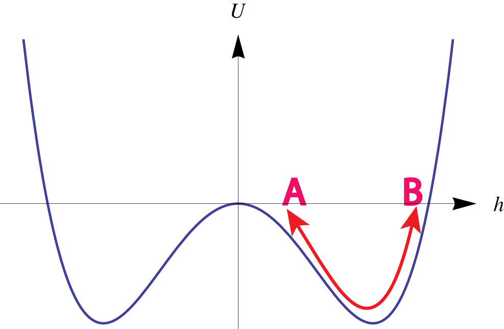
Figure 1: Double well potential $U$ for a classical particle with coordinate $h$. If the particle starts slightly outside of the origin, say at $A$, then the particle will oscillate between $A$ and another point $B$ with the same potential energy.

2.2 The Final Configuration

We have seen that the instability induces an oscillatory solution in the potential (2.14). Suppose that our system is weakly coupled to a heat reservoir with a large heat capacity at very low temperature. Eventually the oscillation will fade away by transferring its energy to the heat reservoir and the system will land on its lowest energy state. Let us try to find out the final configuration of this process.

For the static solutions,

$$h=\pm\frac{1}{2\alpha}\sqrt{\frac{4\alpha E-k}{2k}},$$ (2.15)

which stay at one of the two minima of the potential, the energy density $\mathcal{H}$ is given by

$$\mathcal{H}=U+\frac{1}{2}E^{2}=\frac{k}{4\alpha}\left(E-\frac{k}{8\alpha}\right)\;.$$ (2.16)

Especially, the energy density vanishes when $k=0$. Figure 2 shows the amplitude $h$ and the energy density $\mathcal{H}$ change as functions of $k$. Since the energy density is monotonically increasing in $k$, we expect that solutions with $k\neq 0$ are unstable and decay to the solution with $k=0$. Note that, although $h$ diverges as $k$ goes to $0$, the field strength $E$ vanishes in this limit. The constant electric field in the initial configuration is wiped out in the $k=0$ solution and the final configuration will be the trivial vacuum state with $E=0$.

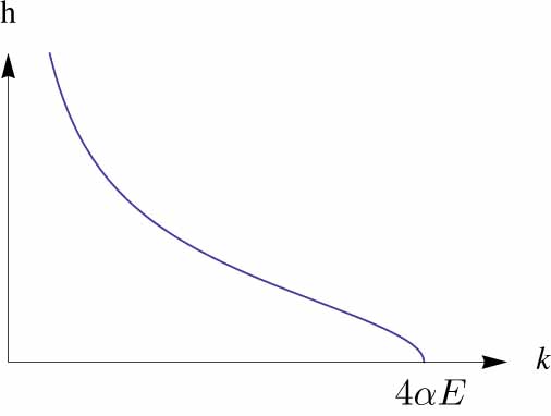
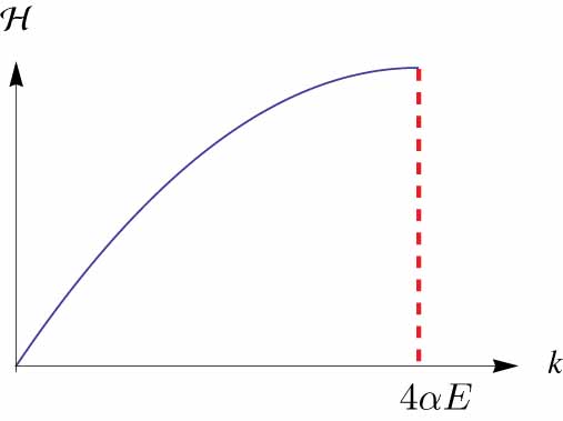
Figure 2: The amplitude $h$ and the energy density $\mathcal{H}$ as a function of $k$.

We can directly check that the static solution (2.15) with $k\neq 0$ is unstable. The solution corresponds to the gauge field configuration, $A_{1}^{(0)}(t)=\frac{k}{4\alpha}t$ and $A_{3}^{(0)}+iA_{4}^{(0)}=\frac{1}{2\alpha}\sqrt{\frac{4\alpha E-k}{2k}}e^{-ikx_{2}}$. Let us add a small perturbation $A^{(0)}\rightarrow A^{(0)}+a$ to this background. Assuming that the modes depend only on $t$ and $x_{2}$ with $a_{0}=0$, the equations of motion become

$$\ \begin{split}\Box a_{1}+2\alpha kh(e^{ikx_{2}}\partial_{0}a_{+}+e^{-ikx_{2}}\partial_{0}\bar{a}_{+})&=0\\ \Box a_{2}&=0\\ \Box a_{+}+ik\partial_{2}a_{+}-4\alpha khe^{-ikx_{2}}\partial_{0}a_{1}&=0\;,\end{split}$$ (2.17)

where $\Box=-\partial_{0}^{2}+\partial_{2}^{2}$ and $a_{+}=a_{3}+ia_{4}$. The coefficients of the equations have $x_{2}$ dependence, which can be removed by using two real variables $\tilde{a}_{3}$ and $\tilde{a}_{4}$ such that $a_{+}=e^{-ikx_{2}}(\tilde{a}_{3}+i\tilde{a}_{4})$ in place of $a$. Assuming the $t$ and $x_{2}$ dependence of the fields $a_{1}$, $\tilde{a}_{3}$ and $\tilde{a}_{4}$ to be of the form $e^{-i\omega t+iqx_{2}}$ and that $a_{2}=0$, a non-trivial solution exists if and only if

$$(\omega^{2}-q^{2})\left[\omega^{4}-2\omega^{2}(q^{2}+k(4\alpha E-k))+q^{2}(q^{2}-k^{2})\right]=0\;,$$ (2.18)

From the second factor, we see that the product of two solutions for $\omega^{2}$ is $q^{2}(q^{2}-k^{2})$, which is negative for $0<q<k$. Thus one of the two roots of $\omega^{2}$ must be negative, representing an unstable mode. Since the momentum $q$ of the instability mode is in the range $0<q<k$, we expect that the solution decays toward the lowest energy state with momentum $k=0$.

We have also performed numerical analysis of time dependent solutions with the initial configuration of constant electric field $E$ assuming that solutions depend only on the coordinates $t$ and $x_{2}$. We found that a small localized perturbation generates a domain where the electric and magnetic fields fluctuate and that the domain expands at the speed of light. The magnetic field in the domain carries a range of momenta, which tend to move to zero momentum state. The strength of the electric field decays as the domain expands, suggesting that the system will eventually settle down to the trivial state with $E=0$.

To summarize, the instability of the constant electric field in the Maxwell-Chern-Simons theory in the 5-dimensional Minkowski space, which we found in our previous paper [1], leads to the trivial vacuum state with no background field strength $F_{IJ}=0$. This reminds us of the Schwinger mechanism where a constant electric field is screened by virtual production of electron-positron pairs.

This result should be contrasted with the corresponding instability of the charged black hole in $AdS_{5}$, which we will study in the next section. There, we do not expect that the background electric field to disappear since the electric charge of the black hole is fixed by the chemical potential at the boundary. Indeed, we will find stable solutions with non-zero momentum $k$ in this case.

3 Maxwell-Chern-Simons Theory in the $AdS_{5}$ Black Hole Geometry

In this section, we will construct non-linear solutions which describe the end-point of the instability of the charged black hole in $AdS_{5}$. Since the Maxwell field contributes to the energy momentum tensor, in general we need to analyze the coupled Einstein and Maxwell equations. Here we will simplify the problem by taking a limit where we can ignore the back-reaction of the Maxwell field to the metric.

The Lagrangian density for the Maxwell-Chern-Simons theory is given by

$$\mathcal{L}=-\frac{1}{4}F_{IJ}F^{IJ}+\frac{\alpha}{3!\sqrt{-g}}\epsilon^{IJKLM}A_{I}F_{JK}F_{LM}\;.$$ (3.1)

Rescaling the gauge field as $\tilde{A}=\alpha A$, the Lagrangian density becomes

$$\mathcal{L}=\frac{1}{\alpha^{2}}\left(-\frac{1}{4}\tilde{F}_{IJ}\tilde{F}^{IJ}+\frac{1}{3!\sqrt{-g}}\epsilon^{IJKLM}\tilde{A}_{I}\tilde{F}_{JK}\tilde{F}_{LM}\right)\;.$$ (3.2)

When $\alpha$ is large, for a solution with finite $\tilde{A}$, the energy-momentum tensor is of the order $O(1/\alpha^{2})$ and the coupling of the Maxwell field to the metric is suppressed. This limit is analogous to the infinite charge limit considered in the holographic description of superconductivity [2].

3.1 The Large $\alpha$ Limit

To keep $\tilde{A}$ finite, we have to scale the background gauge field as well. This means that the chemical potential $\mu$ of the black hole should also be scaled in such a way that the combination $\alpha\mu$ remains finite. Let us examine what this limit means to the black hole solution. The Reissner-Nordström solution has the metric

$$ds^{2}=-H(r)dt^{2}+\frac{1}{H(r)}dr^{2}+r^{2}d{\vec{x}}^{2}\;,\qquad\vec{x}=(x^{2},x^{3},x^{4})\;,$$ (3.3)

where the function $H(r)$ is given by

$$H(r)=r^{2}\left[1-\left(\frac{r_{+}}{r}\right)^{4}\right]\;,$$ (3.4)

The temperature in this limit of $\mu\rightarrow 0$ becomes

$$T=\frac{r_{+}}{2\pi}\left(2-\frac{\mu^{2}}{3r_{+}^{2}}\right)\rightarrow\frac{r_{+}}{\pi}\;.$$ (3.5)

The background geometry in this limit is simply the (neutral) Schwarzschild $AdS_{5}$ solution. In terms of the rescaled finite gauge field $\tilde{A}$, the background field strength is given by

$$\tilde{F}=\frac{\tilde{E}}{r^{3}}dt\wedge dr\;,\qquad\text{where $\tilde{E}=-2\alpha\mu r_{+}^{2}=-\frac{2r_{+}^{3}}{\pi}\frac{1}{\tau}$,}$$ (3.6)

where we introduce a new variable $\tau=r_{+}/\pi\alpha\mu$ for later convenience. Since $\tau=T/{\mu\alpha}$, it can be thought of as a rescaled temperature.

It is important to note that we have access to the phase transition point in this limit. In [1], we studied the instability of the Reissner-Nordström solution and obtained the critical temperature $T_{c}$ for the instability as a function of the Chern-Simons coupling $\alpha$. The result of our numerical analysis is reproduced in Figure 3. For large $\alpha$, the dimensionless combination $T_{c}/\mu$ grows linearly in $\alpha$. Thus, we can analyze the behavior of the system near $T=T_{c}$ by taking the limit of $\alpha\rightarrow\infty$ while keeping the combination $\alpha\mu$ finite.

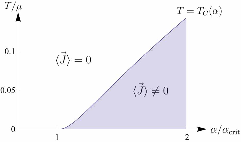
Figure 3: Critical temperature as a function of the Chern-Simons coupling $\alpha$. The shaded region indicates a phase with a non-zero expectation value of the conserved current $\vec{J}$ which is helical and position dependent.

Let us find a non-linear solution to the equations of motion that describes the spatially modulated phase in this limit. We look for a solution that has the same symmetry as that of the unstable modes found in [1], namely a linear combination of a translation along $x_{2}$ and a rotation in the 3-4 plane, as well as the translation symmetries along $t$, $x_{3}$ and $x_{4}$. This leads to the following ansatz,

$$\begin{split}&\tilde{A}_{0}=f(r)\;,\qquad\tilde{A}_{1}=g_{1}(r)\;,\qquad\tilde{A}_{2}=g_{2}(r)\\ &\tilde{A}:=\tilde{A}_{3}+i\tilde{A}_{4}=h(r)e^{-ikx_{2}}\;.\end{split}$$ (3.7)

Note that $g_{1}(r)$ can be set to vanish by a gauge choice, and $g_{2}(r)$ has to vanish by the Maxwell equation $\frac{\delta S}{\delta\tilde{A}_{2}}=0$. The non-trivial equations of motion are

$$\begin{split}-\partial_{r}(r^{3}f^{\prime}(r))-4kh(r)h^{\prime}(r)&=0\\ \partial_{r}(H(r)rh^{\prime}(r))-\frac{1}{r}k^{2}h(r)+4kh(r)f^{\prime}(r)&=0\;.\end{split}$$ (3.8)

The first equation can be integrated and becomes

$$r^{3}f^{\prime}(r)+2kh(r)^{2}=\tilde{E}\;.$$ (3.9)

Eliminating $f^{\prime}(r)$ in the second equation by using the above relation, we obtain

$$\partial_{r}(H(r)rh^{\prime}(r))-\frac{1}{r}k^{2}h(r)+4k\frac{h(r)}{r^{3}}(\tilde{E}-2kh(r)^{2})=0\;.$$ (3.10)

3.2 Second Order Phase Transition

We have solved the differential equation (3.10) numerically. For each initial condition at the horizon, the equation is integrated numerically toward the $AdS_{5}$ boundary. In general, we find a linear combination of normalizable and non-normalizable modes near the boundary. Since the new phase of the system should be represented by a normalizable solution, we tune the initial condition at the horizon so that the non-normalizable component vanishes. Figure 4 describes numerical solutions for $\tau=0.35$. The left graph shows the amplitude $h(r_{+})=h_{0}$ at the horizon as a function of the momentum $k$.

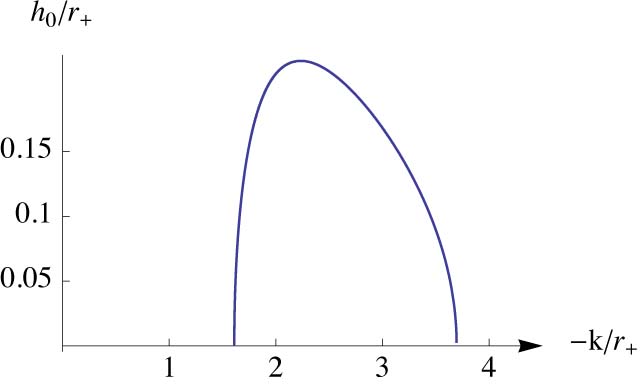
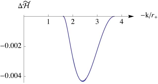
Figure 4: The amplitude $h_{0}$ and the energy density difference $\Delta\widetilde{\mathcal{H}}$ from the homogeneous phase as functions of $k$.

Since there is a family of solutions parametrized by the momentum $k$, we need to choose the minimum energy density solution as the final state. The energy density is given as a sum of the electric and magnetic energy

$$\mathcal{H}=\frac{1}{2\alpha^{2}}\int dr\left[f^{\prime}(r)^{2}+\frac{k^{2}}{r^{4}}h(r)^{2}+\frac{H(r)}{r^{2}}h^{\prime}(r)^{2}\right]\;.$$ (3.11)

It is convenient to rescale the energy density as $\tilde{\mathcal{H}}=\alpha^{2}r_{+}^{4}\mathcal{H}$, which is finite in the limit of $\alpha\rightarrow\infty$. The right graph of Figure 4 shows the energy density as a function of $k$. Choosing the momentum corresponding to the minimum of the energy density, the expectation value of the order parameter $|\left<J_{3}+iJ_{4}\right>|$ can be read off from the asymptotic behavior of the corresponding bulk field $h(r)$. Figure 5 shows the expectation value $|\left<J_{3}+iJ_{4}\right>|$ as a function of the rescaled temperature $\tau$. Near the critical temperature, it behaves as

$$|\left<J_{3}+iJ_{4}\right>|=A\left(1-\frac{\tau}{\tau_{c}}\right)^{\frac{1}{2}}\;,$$ (3.12)

where $A=2.04$ and $\tau_{c}=0.37$. The critical exponent $1/2$ is typical for a mean field theory. Indeed, this can be expected from the absence of quadratic terms in the equations of motion (3.10) and the fact that we consider the gravity system classically. The mean field behavior is also observed in the holographic description of superconductivity [2, 4].

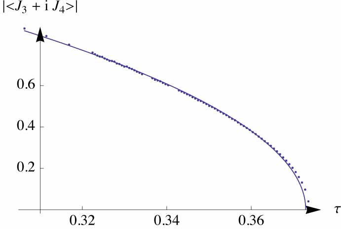
Figure 5: The expectation value of the order parameter as a function of the temperature. The dotted curve is the numerical result and the solid curve is its fit with $(1-\tau/\tau_{c})^{1/2}$.

4 Quantum Corrections

We found that the phase transition is of the second order in the classical supergravity approximation. In this section, we provide evidence that quantum corrections in the bulk change it to the first order. Such a phenomenon has been observed by Brazovskii [5] and elaborated by Swift and Hohenberg in [6], in the context of a classical statistical model at finite temperature. We will extend this result to the gravity theory in $AdS_{5}$.

Let us review the Brazovskii model. It is a classical field theory in $d$ space dimensions at finite temperature with the following scalar field Hamiltonian in the momentum representation,

$$\begin{split}\mathcal{F}=&\frac{1}{2}\int\frac{d^{d}q}{(2\pi)^{d}}\phi(\vec{q})\phi(-\vec{q})\left[m^{2}+(|\vec{q}|-q_{0})^{2}\right]\\ &+\frac{\lambda}{4!}\int\frac{d^{d}q_{1}}{(2\pi)^{d}}\frac{d^{d}q_{2}}{(2\pi)^{d}}\frac{d^{d}q_{3}}{(2\pi)^{d}}\phi(\vec{q}_{1})\phi(\vec{q}_{2})\phi(\vec{q}_{3})\phi(-\vec{q}_{1}-\vec{q}_{2}-\vec{q}_{3})\;.\end{split}$$ (4.1)

Note the unconventional dispersion relation $\omega=m^{2}+(|\vec{q}|-q_{0})^{2}$. It has the Van Hove singularity $d\omega/dq=0$ at $|\vec{q}|=q_{0}$, which will play an important role in the following.

In the mean field approximation, the system undergoes a phase transition at $m^{2}=0$, and there is a spatially modulated phase for $m^{2}<0$. The phase is characterized by the position dependent expectation value of $\phi(\vec{x})$,

$$\left<\phi(\vec{x})\right>=2a\cos\vec{q}\cdot\vec{x}\;,$$ (4.2)

with $|\vec{q}|=q_{0}$. The phase transition is of the second order in this approximation.

Let us examine if this picture is modified by thermal fluctuations. The inverse susceptibility is defined by

$$M^{2}:=G^{-1}(|\vec{q}|=q_{0})=m^{2}-\Sigma(|\vec{q}|=q_{0})\;,$$ (4.3)

where $\Sigma$ represents thermal loop contributions. In the Hartree approximation,

$$M^{2}=m^{2}+\frac{s\lambda}{M}+\lambda a^{2}\;,$$ (4.4)

where $s=\pi S_{d}q_{0}^{d-1}/(2\pi)^{d}$ with $S_{d}$ the area of the $(d-1)$-sphere. There are higher order corrections, but they will not affect the behavior of $M^{2}$ near $a=0$. The first term in the right-hand side of (4.4) is the tree level value. The second term comes from a loop diagram as in Figure 6, which gives a contribution near $q=q_{0}$ of the form

$$\frac{\lambda}{(2\pi)^{d}}\int\frac{d^{d}\vec{q}}{M^{2}+(|\vec{q}|-q_{0})^{2}}\sim\frac{\lambda}{(2\pi)^{d}}S_{d}q_{0}^{d-1}\int_{0}^{\infty}\frac{dq}{M^{2}+(q-q_{0})^{2}}=\frac{\lambda}{(2\pi)^{d}}\frac{\pi S_{d}q_{0}^{d-1}}{M}\;.$$ (4.5)

There are subleading terms for small $M$, but what is relevant for the analysis below is the $1/M$ pole from the loop. The third term $\lambda a^{2}$ comes from the quartic coupling combined with the expectation value (4.2) of $\phi$.

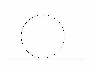
Figure 6: A loop diagram that contributes to the two point correlation function.

The free energy $\mathcal{F}$ for the expectation value (4.2) can be evaluated by setting [5],

$$\frac{d\mathcal{F}}{da}=2M^{2}a-\lambda a^{3}\;.$$ (4.6)

Combining this with

$$\frac{da}{dM}=\frac{M}{\lambda a}\left(1+\frac{s\lambda}{2M^{3}}\right)\;,$$ (4.7)

derived from (4.4), we find

$$\begin{split}\mathcal{F}&=\int\frac{d\mathcal{F}}{da}da=\int\frac{d\mathcal{F}}{da}\frac{da}{dM}dM\\ &=\frac{1}{2\lambda}\left(\frac{M^{4}}{2}+m^{2}M^{2}+3s\lambda M-\frac{s\lambda m^{2}}{M}-\frac{s^{2}\lambda^{2}}{2M^{2}}\right)\;.\end{split}$$ (4.8)

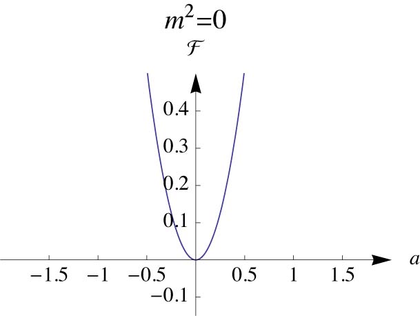
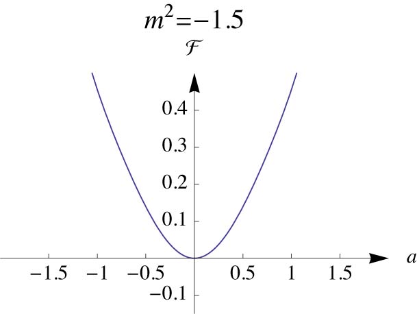
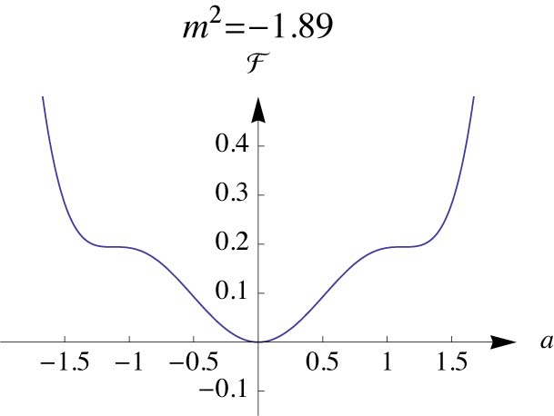
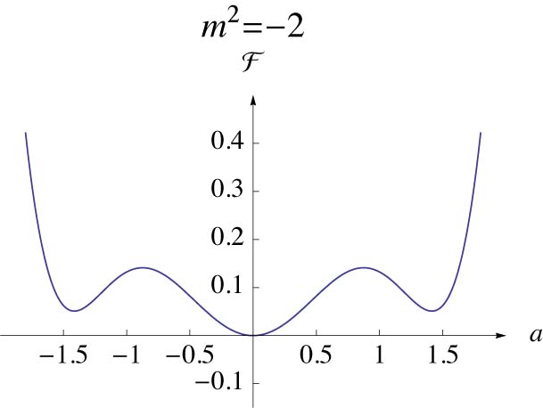
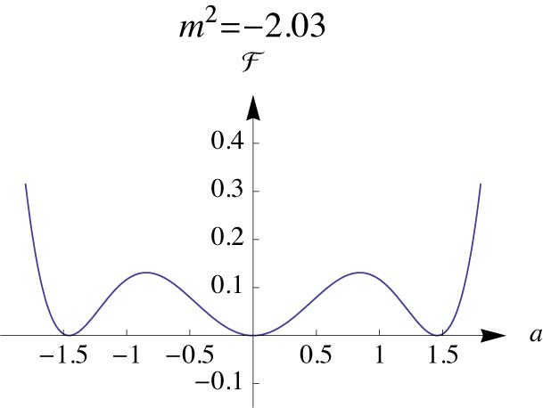
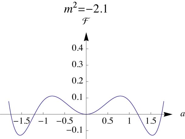
Figure 7: Different shapes of the graphs of the free energy $\mathcal{F}$ as a function of $a$ as the parameter $m^{2}$ changes.

Note that the terms in the parenthesis in (4.8) depend on $s$ and $\lambda$ only in the combination $s\lambda$. If we rescale $m$ and $M$ by a factor of $\epsilon$ and $s\lambda$ by $\epsilon^{3}$, the terms in the parenthesis in (4.8) scales like $\epsilon^{4}$. Thus, we can set $s=\lambda=1$ without loss of generality if we do not care about an overall factor of $\mathcal{F}$. Figure 7 illustrates the free energy $\mathcal{F}$ as a function of $m^{2}$. For $m^{2}\geq 0$, we have a graph with only a minimum at the origin. As $m^{2}$ decreases and crosses $-2^{-\frac{2}{3}}3\sim-1.89$, we see two inflection points away from the origin, representing the spatially modulated phase. At this point, the homogeneous phase at $a=0$ still has a lower energy. As we lower $m^{2}$ further, the energy of the spatially modulated phase becomes lower than that of the homogeneous phase, and the first order phase transition occurs.

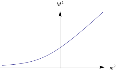
Figure 8: The relation between $m^{2}$ and $M^{2}$. Note that for any value of $m^{2}$, there is always a solution with $M^{2}>0$.

The crucial point is that the origin $a=0$ remains semi-stable throughout the process since $d^{2}\mathcal{F}/da^{2}=2M^{2}>0$ at $a=0$. This in turn is due to the fact that (4.4) has a solution with $M^{2}>0$ for any value of $m^{2}$ including $m^{2}<0$. This is possible since the second term in the equation is proportional to $1/M$ and diverges as $M\rightarrow 0$. This is illustrated in Figure 8. Since $a=0$ is always semi-stable, the phase transition cannot be of the second order.

The $1/M$ singularity in (4.4) originates from the fact that the kinetic operator $\left[M^{2}+(|\vec{q}|-q_{0})^{2}\right]$ vanishes at $M^{2}=0$ and $|\vec{q}|=q_{0}$. If the zero of the kinetic operator were at $\vec{q}=0$, it would not have caused the $1/M$ singularity because the factor $q^{d-1}$ in the phase space volume $q^{d-1}dq$ would have suppressed it. The singularity is generated in our case because of the larger phase space volume $\sim q_{0}^{d-1}dq$ at $|\vec{q}|=q_{0}$ in (4.5). It ensures that there is a positive $M^{2}$ solution to (4.4) and that the origin of the field space is meta-stable.

This feature is shared by the gravity theory considered in this paper. In our classical analysis in the last section, we found that the phase transition happens at $T=T_{c}$ and the new phase for $T<T_{c}$ is represented by the non-linear static solutions constructed in section 3. Since the phase transition is of the second order, the size of the non-linear solution grows linearly in $\sqrt{T_{c}-T}$. This means that, at $T=T_{c}$, there are static solutions to the linearized equations of motion, namely a zero of the kinetic operator at non-zero momenta. As in the case of the Brazovskii model, it generates a $1/M$ singularity in the two-point function. Thus, we expect that the homogeneous phase will remain meta-stable for $T<T_{c}$. If quantum corrections are parametrically suppressed (e.g., by $1/N$), the spatially modulated phase will eventually acquire lower energy and the first order phase transition will take place at that point.

5 Linear response

Finally, let us examine linear response of our solution when we couple a gauge field to the current $J$ at the boundary. Because of the Chern-Simons term, the current is anomalous. We therefore treat the boundary gauge field as an external and non-dynamical source as in recent papers, for example [7, 8].

Note that the background solution we consider is inhomogeneous, carrying the momentum $k$. In the homogeneous setup, it is natural to choose a translationally invariant source. In our case, we consider a small perturbation of the form $\tilde{A}=\tilde{A}^{(0)}+a$, where $\tilde{A}^{(0)}$ is our non-linear solution and $a$ is a small perturbation with non-zero components,

$$a_{3}(x_{2},r,t)+ia_{4}(x_{2},r,t)=-ia_{T}(r,t)e^{-ikx_{2}},~{}~{}~{}a_{2}(r,t)=a_{L}(r,t)\;.$$ (5.1)

Here, $a_{T}(r,t)$ and $a_{L}(r,t)$ are real functions of $r$ and $t$. Notice that we turn on a magnetic field as well as an electric field. It is not possible to turn on only an electric field due to the Bianchi identity $\partial_{[+}F_{t2]}=0$, where $+$ denotes the coordinate $x_{3}+ix_{4}$. However, in the current setup, the magnetic field is determined by the electric field and is not an independent quantity.

The non-trivial linear equations of motion of the fields $a_{T}(r,t)$ and $a_{L}(r,t)$ are

$$\begin{split}-\frac{r}{H(r)}\partial_{t}^{2}a_{L}+\partial_{r}(rH(r)\partial_{r}a_{L})+4\partial_{r}h(r)\partial_{t}a_{T}&=0\\ -\frac{r}{H(r)}\partial_{t}^{2}a_{T}+\partial_{r}(rH(r)\partial_{r}a_{T})-\frac{k^{2}}{r}a_{T}+4k\frac{\tilde{E}-2\alpha kh(r)^{2}}{r^{3}}a_{T}-4\partial_{r}h(r)\partial_{t}a_{L}&=0\;.\end{split}$$ (5.2)

Here $h(r)$ is the non-linear solution we have found previously. We are interested in modes with definite frequency of the form $e^{-i\omega t}$. The fields $a_{T}(r)$ and $a_{L}(r)$ behave as $H(r)^{-\frac{i\omega}{4}}$ near the horizon $r=r_{+}$ if we impose the in-going boundary condition. On the other hand, near the $AdS_{5}$ boundary $r=\infty$, they behave as

$$\begin{split}a_{T}&=a_{T(0)}+a_{T(2)}r^{-2}+a_{T(\log)}r^{-2}\log r/r_{+}+\cdots\\ a_{L}&=a_{L(0)}+a_{L(2)}r^{-2}+a_{L(\log)}r^{-2}\log r/r_{+}+\cdots\;.\end{split}$$ (5.3)

Note that there are logarithmic terms and that the coefficient $a_{T(2)}$ or $a_{L(2)}$ can be shifted by $a_{T(\log)}$ and $a_{L(\log)}$ if we change the scale of the radial coordinate $r$. This corresponds to the choice of a renormalization scale, and should not affect physical quantities. The behavior of the equations (5.2) near the $AdS_{5}$ boundary $r=\infty$ fixes $a_{T(\log)}$ and $a_{L(\log)}$ to be

$$a_{T(\log)}=\frac{1}{2}(\omega^{2}-k^{2})a_{T(0)}\;,\qquad a_{L(\log)}=\frac{\omega^{2}}{2}a_{L(0)}\;.$$ (5.4)

Since we are solving a set of linear differential equations, the coefficients $a_{T(2)}$ and $a_{L(2)}$ are determined linearly from $a_{T(0)}$ and $a_{L(0)}$. That is,

$$\begin{pmatrix}a_{T(2)}\\ a_{L(2)}\end{pmatrix}=\Omega\begin{pmatrix}a_{T(0)}\\ a_{L(0)}\end{pmatrix}\;,$$ (5.5)

for some $2\times 2$ complex matrix $\Omega$. From the prescription in [9], and analogously to [10], the retarded Green’s functions for fields $a_{T}$ and $a_{L}$ are given by

$$G^{R}=2\Omega+\begin{pmatrix}\left(\omega^{2}-k^{2}\right)\left(\log\frac{r}{r_{+}}-\frac{1}{2}\right)&0\\ 0&\omega^{2}\left(\log\frac{r}{r_{+}}-\frac{1}{2}\right)\end{pmatrix}\;,$$ (5.6)

where the last term is due to the logarithmically divergent terms in (5.3) whose coefficients are given in (5.4). These divergent parts can be removed by adding a suitable boundary counterterm to the gravity action. After subtracting the divergence, we arrive at

$$G^{R}=2\Omega-\begin{pmatrix}\frac{1}{2}\left(\omega^{2}-k^{2}\right)&0\\ 0&\frac{1}{2}\omega^{2}\end{pmatrix}\;,$$ (5.7)

When considering modes of definite frequency, the additional electric fields $E_{T}$ and $E_{L}$ are $i\omega a_{T(0)}$ and $i\omega a_{L(0)}$, respectively. Therefore the conductivity is given by

$$\sigma=\frac{1}{i\omega}G^{R}=\frac{2}{i\omega}\Omega+\begin{pmatrix}\frac{i}{2\omega}\left(\omega^{2}-k^{2}\right)&0\\ 0&\frac{i\omega}{2}\end{pmatrix}\;.$$ (5.8)

Let us evaluate the conductivity $\sigma$ numerically for the Chern-Simons coupling $\alpha=0.59$. For this value of $\alpha$, the minimum energy occurs at the momentum $k=-2.37r_{+}$. We denote the components of the retarded Green’s function and the conductivity respectively as

$$G^{R}=\begin{pmatrix}G_{TT}&G_{TL}\\ G_{LT}&G_{LL}\end{pmatrix}\;,$$ (5.9)

and

$$\sigma=\begin{pmatrix}\sigma_{TT}&\sigma_{TL}\\ \sigma_{LT}&\sigma_{LL}\end{pmatrix}\;.$$ (5.10)

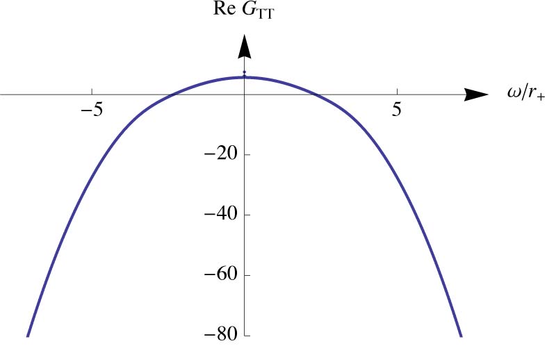
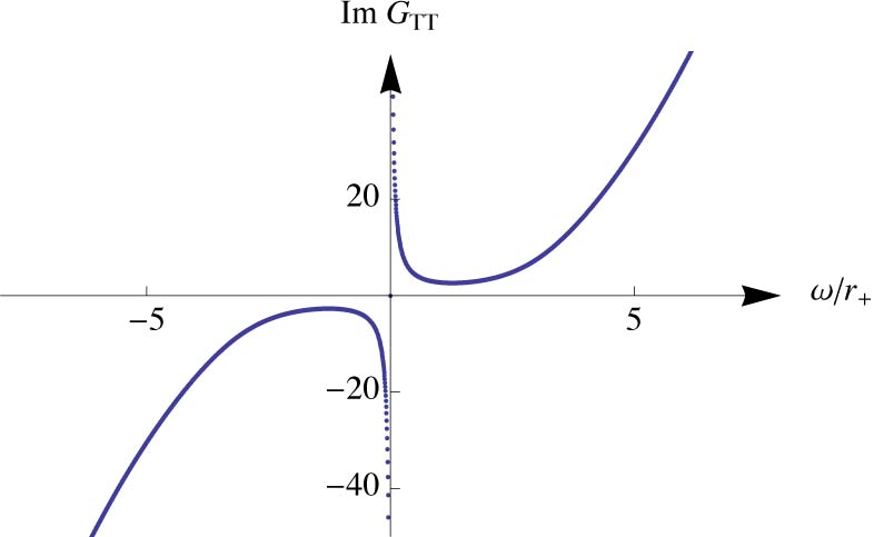
Figure 9: The real and the imaginary parts of $G^{R}_{TT}$.

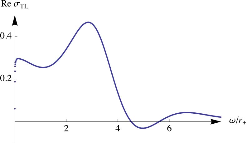
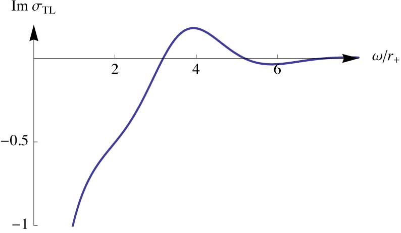
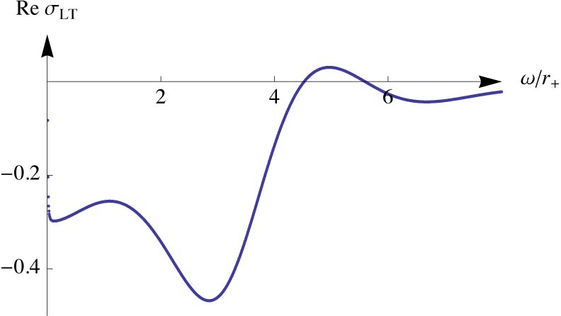
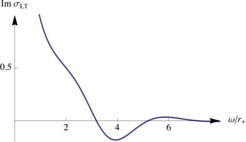
Figure 10: The real and the imaginary parts of $\sigma_{TL}$ and $\sigma_{LT}$.

This numerical result has several interesting features. The imaginary part of the retarded Green’s function $G_{TT}$ for a pair of $a_{T}$ fields behaves like $1/\omega$ near $\omega=0$, as shown in Figure 9. The pole at $\omega=0$ is directly related to the fact that $a_{T}$ is a Goldstone mode. This can be seen as follows. As $\omega$ goes to 0, the solution becomes static and we can ignore the terms with time derivatives in (5.2). In this limit, the equation of motion for $a_{T}$ reduces to the linearized version of the equation for the phase rotation of the inhomogeneous background solution (3.7). Especially, $a_{T}$ goes to $h(r)$ as we take a static limit. Since $h(r)$ is a solution that does not have a non-normalizable mode, if we start with a source such that $a_{T(0)}=0$, (5.5) implies that $\Omega_{TT}$ should diverge in the static limit. Therefore, we expect to see a pole at $\omega=0$ in $G^{R}_{TT}$.

Figure 10 shows the off-diagonal components of the conductivity $\mathrm{Im}\,\sigma_{TL}$ and $\mathrm{Im}\,\sigma_{LT}$. Note that they behave as $1/\omega$ with opposite coefficients. The antisymmetry of $\sigma_{TL}$ and $\sigma_{LT}$ is due to the fact that (5.2) remains invariant under the change $t\rightarrow-t$ if we simultaneously change the sign of $a_{T}(r)$. The poles at $\omega=0$ in the imaginary part of the conductivity indicate that there are delta function contributions at $\omega=0$ to $\mathrm{Re}\,\sigma_{TL}$ and $\mathrm{Re}\,\sigma_{LT}$, which implies that there is an off-diagonal infinite DC conductivity.

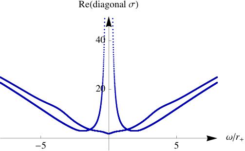
Figure 11: The real parts of the diagonal components of the diagonalized conductivity matrix.

It is also instructive to diagonalize the conductivity matrix. Figure 11 shows the real parts of the two diagonal components of the diagonalized conductivity matrix. The real part of a conductivity is directly related to the spectral density, and the real parts of the two eigenvalues measure the spectral densities corresponding to two linear combinations of the transverse and longitudinal currents associated with $a_{T}$ and $a_{L}$ fields. In particular it should always be positive, and indeed this is shown explicitly in Figure 11. One of the diagonal conductivities has a $1/\omega^{2}$ pole, which is again related to the presence of a Goldstone mode.

Appendix A Analysis in the $AdS_{2}\times\mathbb{R}^{3}$ geometry

In this appendix, we consider the Maxwell field in the $AdS_{2}\times\mathbb{R}^{3}$ geometry ignoring its back-reaction to the metric. Since the geometry corresponds to the zero temperature limit of the black hole, it does not appear in the limit we consider in section 3. On the other hand, the equations of motion can be solved analytically in this case, and it gives a natural generalization of the analysis in section 2.

The metric of $AdS_{2}\times\mathbb{R}^{3}$ is given by

$$ds^{2}=-r^{2}dt^{2}+\frac{dr^{2}}{r^{2}}+dx_{2}^{2}+dx_{3}^{2}+dx_{4}^{2}\;.$$ (A.1)

Note that, especially, $\sqrt{-g}=1$. We assume the radius of curvature for $AdS_{2}$ is 1. A different value of the radius can be easily considered by using dimensional analysis. For a generic metric, the Lagrangian is given by

$$\mathcal{L}=-\frac{1}{4}F_{IJ}F^{IJ}+\frac{\alpha}{3!\sqrt{-g}}\epsilon^{IJKLM}A_{I}F_{JK}F_{LM}\;,$$ (A.2)

whose equation of motion is

$$\partial_{J}(\sqrt{-g}F^{JI})+\frac{\alpha}{2}\epsilon^{IJKLM}F_{JK}F_{LM}=0\;.$$ (A.3)

The index is such that $t=0$ and $r=1$. Here $\sqrt{-g}=1$.

Let us find out a class of non-linear static solutions with the ansatz

$$\begin{split}&A_{0}=f(r)\;,\qquad A_{1}=A_{2}=0\\ &A:=A_{3}+iA_{4}=h(r)e^{-ikx_{2}}\;.\end{split}$$ (A.4)

The equations of motion can be written as

$$\begin{split}-f^{\prime\prime}(r)-4\alpha kh(r)h^{\prime}(r)&=0\\ \partial_{r}(r^{2}h^{\prime}(r))-k^{2}h(r)+4\alpha kh(r)f^{\prime}(r)&=0\;.\end{split}$$ (A.5)

Integrating the first equation, we obtain

$$f^{\prime}(r)+2\alpha kh(r)^{2}=E$$ (A.6)

where $E$ is the constant electric background field since the left hand side is just the first component of the conjugate momentum $\Pi_{1}$. Solving for $f^{\prime}(r)$ and plugging into (A.5),

$$\partial_{r}(r^{2}h^{\prime}(r))-k^{2}h(r)+4\alpha kh(r)(E-2\alpha kh(r)^{2})=0\;.$$ (A.7)

For $u=\log r$, the equation becomes

$$h^{\prime\prime}(u)+h^{\prime}(u)-k^{2}h(u)+4\alpha kh(u)(E-2\alpha kh(u)^{2})=0\;,$$ (A.8)

If we treat $u$ as a time coordinate, this equation describes a one-dimensional motion of a particle parametrized by $h$ subject to a frictional force and under the potential

$$U=\frac{1}{2}k(4\alpha E-k)h^{2}-2\alpha^{2}k^{2}h^{4}\;.$$ (A.9)

If $0<k<4\alpha E$, the potential is an upside-down Mexican hat. If a particle starts at one of the two hills at $u=-\infty$, it will oscillate around $h=0$, as in the case of the Minkowski space discussed in section 2. The new feature in the $AdS_{2}$ case is that there is a friction term in (A.8) and the motion will eventually stop at $h=0$.

In order for a non-linear solution to exist, the momentum $k$ must obey the additional condition, $k(k-4\alpha E)>-\frac{1}{4}$, which is equivalent to the Breitenlohner-Freedman bound. This condition is needed since any non-linear solution $h$ tends to $h=0$ for large $u=\log r$ and obeys the linearized equation near the boundary of $AdS_{2}$. This in particular means that there is no non-linear solution with $k=0$. Unlike the case of the Minkowski space, the end-point of the instability is not a trivial vacuum but a non-trivial solution carrying a non-zero momentum.

References

- [1] S. Nakamura, H. Ooguri and C. S. Park, “Gravity Dual of Spatially Modulated Phase,” Phys. Rev. D 81, 044018 (2010) [arXiv:0911.0679 [hep-th]].
- [2] S. A. Hartnoll, C. P. Herzog and G. T. Horowitz, “Building a Holographic Superconductor,” Phys. Rev. Lett. 101, 031601 (2008) [arXiv:0803.3295 [hep-th]].
- [3] S. Sachdev, “Holographic metals and the fractionalized Fermi liquid,” [arXiv:1006.3794 [hep-th]].
- [4] S. A. Hartnoll, C. P. Herzog and G. T. Horowitz, “Holographic Superconductors,” JHEP 0812, 015 (2008) [arXiv:0810.1563 [hep-th]].
- [5] S. A. Brazovskii, “Phase transition of an isotropic system to a nonuniform state,” Sov. Phys. JETP, 41, 85 (1975).
- [6] J. Swift and P. C. Hohenberg, “Hydrodynamic fluctuations at the convective instability,” Phys. Rev. A, 15, 319 (1977).
- [7] D. T. Son and P. Surowka, “Hydrodynamics with Triangle Anomalies,” Phys. Rev. Lett. 103, 191601 (2009) [arXiv:0906.5044 [hep-th]].
- [8] E. D’Hoker and P. Kraus, “Charged Magnetic Brane Solutions in AdS5 and the fate of the third law of thermodynamics,” JHEP 1003, 095 (2010) [arXiv:0911.4518 [hep-th]].
- [9] D. T. Son and A. O. Starinets, “Minkowski-space correlators in AdS/CFT correspondence: Recipe and applications,” JHEP 0209, 042 (2002) [arXiv:hep-th/0205051].
- [10] G. T. Horowitz and M. M. Roberts, “Holographic Superconductors with Various Condensates,” Phys. Rev. D 78, 126008 (2008) [arXiv:0810.1077 [hep-th]].