Interface Energy in the Edwards-Anderson model

Abstract

We numerically investigate the spin glass energy interface problem in three dimensions. We analyze the energy cost of changing the overlap from $-1$ to $+1$ at one boundary of two coupled systems (in the other boundary the overlap is kept fixed to $+1$). We implement a parallel tempering algorithm that simulates finite temperature systems and works with both cubic lattices and parallelepiped with fixed aspect ratio. We find results consistent with a lower critical dimension $D_{c}=2.5$. The results show a good agreement with the mean field theory predictions.

I Introduction

It is by now a well-established fact (numerically) that spin glass models with nearest neighbour interactions have a finite transition temperature in spatial dimension $D=3$ at zero magnetic field HPV , moreover the predictions of broken replica theory are well in agreement with the numerical data JANUS . However the value of the lower critical dimension $D_{c}$, i.e. the dimension above which there is a phase transition at strictly positive temperature, is still debated and there have been different predictions based on different approaches. The initial investigations, in the framework of the droplet approach, used the stiffness exponent $\theta$ to conclude that, at zero temperature, $\theta>0$ in $D=3$ and $\theta<0$ in $D=2$, thus implying $2<D_{c}<3$ BM . The absence of a transition in $D=2$ was confirmed also by direct numerical simulations D2 , that strongly suggest that the lower critical dimension is greater than 2.

A recent numerical study by Boettcher B reached the conclusion that $D_{c}=2.5$ by measuring the stiffness exponent in various dimensions and making a best fit for its dimensional dependence which gives $\theta=0$ for $D_{c}=2.5$.

An alternative approach has been put forward by Franz, Parisi, Virasoro in FPV . Here to measure the stability of the low temperature spin-glass phase against thermal fluctuations, the energy cost associated to imposing a different value of the overlap along one spatial direction has been considered. Remarkably FPV founds, using an analytical computation based on a mean-field approximation, the same result of the stiffness approach, i.e. $D_{c}=2.5$.

However the approach introduced in FPV has not yet been tested on a finite-dimensional model. This is the aim of this work. We find numerical results compatible with the prediction $D_{c}=2.5$, even though strong finite size effects prevent a final answer.

II Theoretical prediction

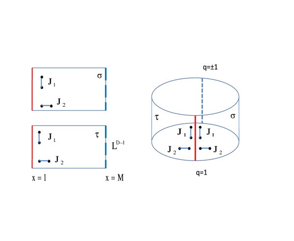
Figure 1: From two copies of longitudinal size $M$ to one system of longitudinal size $2(M-1)$.

We first recall the approach of FPV . We consider two identical copies (same disorder) of a system constrained to have their mutual overlaps on the boundaries fixed to some preassigned values. More precisely, we take two systems with the parallelepiped geometry of Fig. (1). Each system has a base area $L^{D-1}$ and height $M$; we denote by $x$ the coordinate along the longitudinal direction of length $M$. The study of systems with different aspect ratio $R$ for determining the interface exponent has been used in the past VARI . Each of the two systems has free boundary conditions along the longitudinal direction and periodic boundary conditions along the transverse direction. However the two systems are coupled by the value of the overlap at their boundary planes. We compare the following two situations. In the first case, which we call $(++)$ coupling condition, we impose an overlap $+1$ on both the left $(x=1)$ and the right $(x=M)$ boundary plane; in the second case, called here the $(+-)$ coupling condition, the overlap on the left boundary $(x=1)$ is equal to $+1$ and the overlap on the right boundary $(x=M)$ is equal to $-1$. The quantity that we will be interested in is the difference of free energies between the two cases

$$\Delta F=-\frac{1}{\beta}Av(\log Z_{+-}-\log Z_{++})$$ (1)

where $\beta$ is the inverse critical temperature, $Av(-)$ denotes the average over the random couplings and

$$Z_{ab}=\sum_{\sigma\tau}e^{-\beta(H_{\sigma}+H_{\tau})}\delta\left(\frac{1}{L^{D-1}}\sum_{i\in A_{1}}{\sigma_{i}\tau_{i}-a}\right)\delta\left(\frac{1}{L^{D-1}}\sum_{i\in A_{M}}{\sigma_{i}\tau_{i}-b}\right)$$ (2)

with $a,b\in\{\pm\}$ and $A_{1}$ (resp. $A_{M}$) the left (resp. right) boundary plane, $H_{\sigma}$ the Hamiltonian of the spin configuration $\sigma$. One can prove that $\Delta F$ is a positive quantity thanks to the fact that $Z_{+,+}\geq Z_{+,-}$. Thus Eq. (1) seems an appropriate definition of a domain wall in spin glass models, in full analogy with usual ferromagnetic systems where a positive domain wall is obtained by imposing different values of the magnetization along one spatial direction.

Since free energies are not directly accessible through Monte Carlo methods BM ; BFP , in our simulations we measured the differences of internal energies between the $(+-)$ and $(++)$ case

$$\Delta E=Av(E_{+-}-E_{++})$$ (3)

where

$$E_{ab}=\sum_{\sigma\tau}(H_{\sigma}+H_{\tau})\frac{e^{-\beta(H_{\sigma}+H_{\tau})}\delta\left(\frac{1}{L^{D-1}}\sum_{i\in A_{1}}{\sigma_{i}\tau_{i}-a}\right)\delta\left(\frac{1}{L^{D-1}}\sum_{i\in A_{M}}{\sigma_{i}\tau_{i}-b}\right)}{Z_{ab}}.$$ (4)

We observe that at zero temperature $\Delta E=\Delta F$. Thus, at small enough temperatures, the positivity of $\Delta E$ follows from the positivity of $\Delta F$ by a continuity argument. However we remark that in our numerical simulations we found always positive energy differences at all temperatures. More precisely, for a random initial condition, the sign of $E_{+-}-E_{++}$ fluctuates at the beginning of the Monte Carlo run and then it stabilizes to a positive sign.

For many models FPV we observe that, below the critical temperature, the free energy cost, as a function of the transverse and longitudinal length, scales for large volumes as $\Delta F\sim L^{D-1}M^{-\omega}$ with $\omega$ independent from the dimension (for $T>T_{c}$, $\Delta F\sim\exp(-L)$). The scaling of the free energy cost defines a lower critical dimension $D_{c}$ in the usual way: for an assigned aspect ratio $R=M/L$ the free energy cost behaves as $\Delta F\sim L^{D-1-\omega}$. From this expression we see that the lower critical dimension, the one above which $\Delta F$ increases with $L$ and below which it vanishes with $L$, turns out to be $D_{c}=\omega+1$. The mean-field computation of FPV predicts $D_{c}=5/2$, i.e. $\Delta F\sim L^{D-1}M^{-3/2}$. In other words, below the critical temperature, the free energy cost divided by the volume $V$ turns out to be independent from $L$ and, for large $L$, it scales as

$$\beta\Delta F/V\approx M^{-5/2}f(\beta).$$ (5)

Since the free energy difference and the internal energy difference scale with the same exponent below the critical temperature then we also have

$$\Delta E/V\approx M^{-5/2}f^{\prime}(\beta).$$ (6)

Generally speaking, at the phase transition point one usually obtains by changing the boundary conditions that

$$\Delta F\to C\neq 0.$$

Using Widom’s scaling one gets:

$$\frac{\Delta E}{V}\sim M^{-3+1/\nu}.$$ (7)

In a given case there could be cancellations and $\Delta F$ at the critical point could go to zero with the volume if $C=0$. In ref. BFP it was shown by an explicit computation that this does not happen, at least in the mean field case. We expect that $C$ is a smooth function of the dimension, so that $C=0$ in $D=3$, would be surprising.

III Numerical implementation

In our simulations we have considered the above mentioned geometrical set-up for the case of the Edwards-Anderson Hamiltonian with dichotomic ($\pm 1$) symmetrically distributed random couplings. In particular, the implementation of the two systems coupled at their boundaries was obtained considering a parallelepiped with doubled size in the longitudinal direction. Denoting by $y$ the coordinate in the longitudinal direction of the doubled parallelepiped, the disorder variables are symmetric with respect to the central plane $y=M$. The sub-systems in the half-volumes $y<M$ and $y>M$ interact in the following way (see Fig (1)):

i) to keep the overlap of the spins $\sigma$ and $\tau$ on the old $x=1$ plane fixed to $+1$, the spins of the new doubled system are identified and they lie on the plane $y=M$;

ii) to keep the overlap of the spins $\sigma$ and $\tau$ on the old $x=M$ plane fixed to either $\pm 1$, the spins of the new doubled system at position $y=1$ and $y=2M-1$ are identified. The strength of the couplings among the spins inside those planes are reduced by a factor one-half (in order to have un-biased interactions); the couplings between nearest neighbors not lying inside those planes are flipped when going from the $(++)$ case to the $(+-)$.

Note that the effective longitudinal size of the total system is $2(M-1)$.

IV Results

The data that we are going to describe concern systems with sizes $4\leq L\leq 10$ for the cubic lattice whereas $4\leq L\leq 8$ and $4\leq M\leq 25$ for the parallelepiped lattice (see Tab. 1) and with $30$ different values of the aspect ratio $R=M/L$, ranging from $0.57$ up to $6.25$. The computations have been performed implementing a multi-spin coding of the parallel tempering algorithm with 33 equally spaced temperatures ranging between 0.6 and 2.2.

L	M	sweeps	sample
4	4	8192	9600
	5	8192	6400
	7	8192	6400
	9	32768	6400
	13	262144	3200
	17	1048576	3200
	21	4194304	3200
	25	4194304	2560

L	M	sweeps	sample
6	4	8192	6400
	5	8192	9600
	6	8192	6400
	7	8192	6400
	9	8192	6400
	13	32768	3200
	17	131072	1920
	21	1048576	1920
	25	2097152	1280

L	M	sweeps	sample
7	4	8192	6400
	5	8192	6400
	7	8192	6400
	9	8192	6400
	13	65536	6400
	17	524288	3200
	21	8388608	1280
	25	8388608	1280

L	M	sweeps	sample
8	5	8192	6400
	7	8192	6400
	9	8192	6400
	13	65536	3200
	17	524288	1920

Table 1: System size parameters for the numerical simulations.

We start from the analysis of a cubic lattice ($M=L$). The data for the extensive internal energy difference as a function of temperature for different system sizes are shown in Fig. (2). Below the critical temperature $T_{c}\approx 1.15$ the data vary weakly with the linear lattice size $L$. The theoretical prediction would have been $\Delta F\sim L^{0.5}$. This suggested that there might be strong finite size effects on the energy interface cost for the small lattices we consider.

This is confirmed by the analysis around the critical temperature which is displayed in Fig. (3). For the parallelepiped geometry, the extensive internal energy interface cost shows a different behavior when plotted versus the aspect ratio $R=M/L$ or against the “corrected” aspect ration $\tilde{R}=(M-1)/L$ (see the panels (a) and (b) of Fig. (3)). Even though these two characterizations of the aspect ratios are totally equivalent in the thermodynamic limit, the data show a marked difference in the two cases. To better appreciate this difference we show in the lower panels (c) and (d) of Fig. (3) the same data multiplied by $e^{AR}$ on the left and $e^{A\tilde{R}}$ on the right, where $A=0.77$ has been computed fitting to an exponential form the behavior of the data at large $R$ (or $\tilde{R}$, it gives the same $A$). We do not claim an exponential dependence, we merely used the exponential re-scaling from the fit to make the data variation more visible.

To extract sensible information from our data, a careful analysis of the dependence of $\Delta E$ from $L$ and $M$ is required. Fig. (3) tell us that it is difficult to make an analysis of the data as a function of the aspect ratio CBM . Thus we start from the expected behavior of very large systems

$$\Delta E\sim L^{2}f(M)$$

which is suggested by the general argument that each of the $L^{2}$ spins on each plane give the same contribution. Thus, for the small finite systems we have, we study the dependence on $1/L$ for a fixed $M$. Since we want to study the behavior for systems with longitudinal size much smaller than transverse size, we must limit the analysis to small values of $M$.

At critical temperature we expect the scaling of Eq. (7), i.e.

$$\frac{\Delta E}{L^{2}}\sim M^{-2+1/\nu}$$

Figure (4) shows that $\frac{\Delta E}{L^{2}}(M-1)^{1.43}$ does not depend on $L$ for large $L$ values. This implies a value of $1/\nu=0.57$ to be compared to $1/\nu=0.408$ of HPV . The predicted value of our exponent should be $1.75$. We think that the difference between $2.45$ and the predicted value ($1.75$) is not worrisome given the fact that the value of $\nu$ was computed in HPV using lattices (up to $40^{3}$) that are much larger of ours and, historically, previous determinations of $1/\nu$ on smaller lattices gave large values of $1/\nu$.

Below the critical temperature we expect the scaling of Eq. (6), i.e.

$$\frac{\Delta E}{L^{2}}\sim M^{-3/2}$$

In Fig. (5) we show $\frac{\Delta E}{L^{2}}(M-1)^{3/2}$ versus $1/L$. The behavior is described by a fit of the form $a_{M}+\frac{b_{M}}{L}$. The slope $b_{M}$ is increasing with $M$ while the intercept $a_{M}$ is instead constant in $M$. In Fig. (6) we show $a_{M}(M-1)^{-3/2}$ versus $M-1$ in log-log scale. The data nicely fall on a straight line with a constant slope $a$. The best fit on $b_{M}$ gives $k(M-1)^{-\delta}+h$ with $k<0$ and $\delta=-0.22$ if $M\in\{4,5,7,9,13\}$ while $\delta=-1/2$ excluding the values $M\geq 9$. Thus it would imply that the correction $\frac{b_{M}}{L}$ converges to zero for large volumes with an assigned aspect ratio.

Summarizing, we have found that in the regime $M<<L$ the data for $\Delta E$ are well described by the following behavior

$$\Delta E\sim L^{2}(M-1)^{-3/2}\left(a+\frac{b_{M}}{L}\right)$$

which is compatible with the prediction $D_{c}=2.5$.

It would nice to study the scaling property of the interface energy as a function of both variables $L,M$. In particular one would like to study the dependence when both $L$ and $M$ grow with a fixed aspect ratio. In Fig. (7) we plot $\frac{\Delta E}{L^{2}}(M-1)^{3/2}$ versus $(M-1)/L$ at temperature $T=0.6$. We see that there is not a global clear scaling of the data. We tried also the aspect ratio scaling in the spirit of CBM , according to which $\Delta E=c_{0}(R)L^{\theta_{0}(R)}$. We found very large oscillations in the exponent $\theta_{0}$. We tried to cure the finite size effects by considering the scaling $\Delta E=\left(c_{0}(R)+\frac{c_{1}(R)}{L}\right)L^{\theta_{1}(R)}$ but we have too few points and the final errors have a too large error. One would need larger lattices and smaller errors on the data to reach a definite conclusion.

At this stage it is difficult to assign a precise error on $\omega$ because of the limited range of $L$ ($4-10$); for such small lattices it would be mandatory to consider corrections to scaling and the fits would become unstable.

Acknowledgments: we thank E.Brezin and S.Franz for interesting discussions.

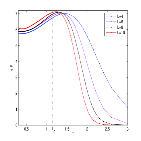
Figure 2: Cubic lattice: extensive internal energy cost of an interface versus the temperature.

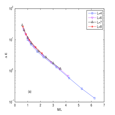
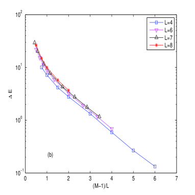
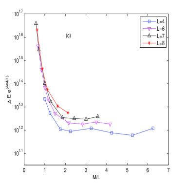
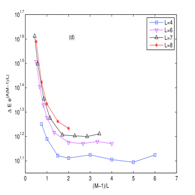
Figure 3: $\Delta E$ as a function of $M/L$ (panel (a)) and as a function of $(M-1)/L$ (panel (b)) at temperature $T=1.1$; $\Delta Ee^{AM/L}$ as a function of $M/L$ (panel (c)) and $\Delta Ee^{A(M-1)/L}$ as a function of $(M-1)/L$ (panel (d)). $A$ is $0.77$. In each panel the different curves refer to different $L$ values.

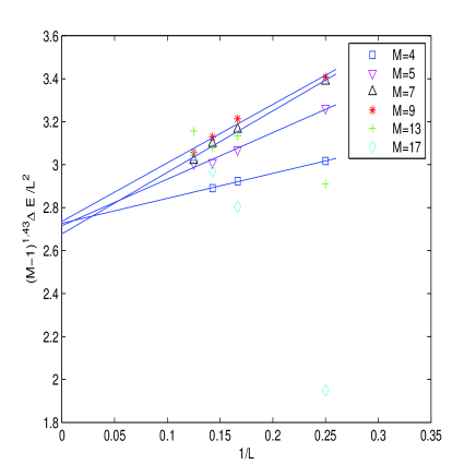
Figure 4: $\frac{\Delta E}{L^{2}}(M-1)^{1.43}$ versus $1/L$ at temperature $T=T_{c}$.

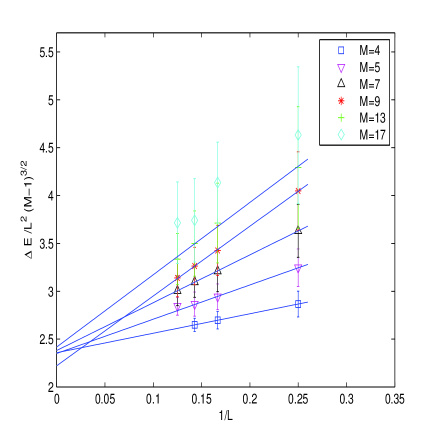
Figure 5: $\frac{\Delta E}{L^{2}}(M-1)^{3/2}$ versus $1/L$ at temperature $T=0.6$.

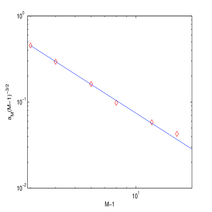
Figure 6: The intercepts of Fig. (5) as a function of $M-1$ at temperature $T=0.6$ in log-log scale. The straight line is the best fit of the form $a(M-1)^{-3/2}$.

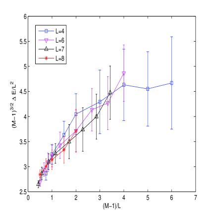
Figure 7: $\frac{\Delta E}{L^{2}}(M-1)^{3/2}$ versus $(M-1)/L$ at temperature $T=0.6$.

References

- (1) S. Boettcher, Stiffness of the Edwards-Anderson model in all dimensions, Phys. Rev. Lett. 95 197205 (2005)
- (2) A.J.Bray and M.A.Moore, Lower critical dimension of Ising spin glasses: a numerical study, J. Phys. C: Solid State Phys., Vol. 17 L463-L468 (1984).
- (3) E. Brézin, S. Franz, G. Parisi, Critical interface: twisting spin glasses at , Phys. Rev. B 82 144427 (2010).
- (4) A.C. Carter, A.J. Bray, M.A. Moore, Aspect-ratio scaling and the stiffness exponent for Ising spin glasses, Phys. Rev. Lett. 88 77201 (2002)
- (5) M. Hasenbusch, A. Pelissetto, E. Vicari, The critical behavior of 3D Ising spin glass models: universality and scaling corrections, J. Stat. Mech.: Theory and Experiment, L02001 (2008)
- (6) S. Franz, G.Parisi, M.A. Virasoro, Interfaces and lower critical dimension in a spin glass model, J. Phys. I France, 4 1657–1667 (1994).
- (7) Alexander K. Hartmann, Alan J. Bray, A.C. Carter, M.A. Moore, A.P. Young, The stiffness exponent of two-dimensional Ising spin glasses for non-periodic boundary conditions using aspect-ratio scaling, Phys. Rev. B 66, 224401 (2002).
- (8) R. Alvarez Banos, A. Cruz, L.A. Fernandez, J. M. Gil-Narvion, A. Gordillo-Guerrero, M. Guidetti, A. Maiorano, F. Mantovani, E. Marinari, V. Martin-Mayor, J. Monforte-Garcia, A. Munoz Sudupe, D. Navarro, G. Parisi, S. Perez-Gaviro, J. J. Ruiz-Lorenzo, S.F. Schifano, B. Seoane, A. Tarancon, R. Tripiccione, D. Yllanes,Nature of the spin-glass phase at experimental length scales arXiv:1003.2569
- (9) J. Lukic, A. Galluccio, E. Marinari, Olivier C. Martin, G. Rinaldi Critical thermodynamics of the two-dimensional +/-J Ising spin glass Physical Review Letters 92 (2004) 117202