Born-Infeld electrostatics in the complex plane

Abstract

The complex method to obtain 2-dimensional Born-Infeld electrostatic solutions is presented in a renewed form. The solutions are generated by a holomorphic seed that makes contact with the Coulombian complex potential. The procedure is exemplified by solving the Born-Infeld multipolar configurations. Besides, it is shown that the attractive force between two equal but opposite charges is lower than its Coulombian partner; it decreases up to vanish when the charges approach each other below a distance ruled by the Born-Infeld constant.

I Introduction

Born-Infeld electrodynamics was born as a non-linear extension of Maxwell’s equations able to render finite the self-energy of the point-like charge B -BI4 . After decades of relative oblivion, Born-Infeld theory regained a prominent place in theoretical physics because of its role in the low energy dynamics of strings and branes Frad -Tsey2 . Born-Infeld theory is distinguished as the only extension of Maxwell’s theory having causal propagation Pleb ; Deser and absence of birefringence Boillat ; Novello . While its free plane waves do not differ from Maxwell’s ones, the Born-Infeld non-linearity provides interactions among plane waves barba ; ferr or between plane waves and static fields Pleb ; Boillat ; 5pleb ; Aiello ; ferr2 ; gibbons that substantially change the physics of propagation. Born-Infeld electrodynamics possesses a magnitude $b$ with units of field that rules the scale of field at which Maxwell’s theory is recovered (in the same way that $c$ rules the Newtonian limit of relativistic mechanics). In this paper we will continue the program to obtain Born-Infeld electrostatic solutions in the Euclidean plane. This program began very early with the articles by Pryce Pryce1 ; Pryce2 , who used the complex analysis to establish the main features of the electrostatic configurations for isolated point-like charges. In Sections 2 and 3 we will present the complex method to generate 2-dimensional electrostatic solutions in a renewed and cleaner way. Recently, the multipolar configurations were worked out Fer ; these solutions displayed some physically undesirable features that will be healed in Sections 5 and 6. Particular features of the dipole field are examined in Sections 7-9, together with general complex expressions for Born-Infeld electrostatic forces and energies. Section 10 describes the solution for two separated equal but opposite charges. It is shown that the attractive force reaches a maximum value at a non-null distance, and then it decreases up to vanish when the charges meet together. Some important characteristics of the holomorphic functions that generate Born-Infeld solutions for point-like charges are discussed in Sections 10 and 11.

II Born-Infeld theory

Like Maxwell’s theory, vacuum Born-Infeld electrodynamics is summarized in two equations:

$$dF\,=\,0\ ,$$ (1)

$$d\ast\mathcal{F}\,=\,0\ .$$ (2)

The 2-form $F$ is the electromagnetic field, and $\mathcal{F}$ is the 2-form

$$\mathcal{F}\ \equiv\ \frac{F-\frac{P}{b^{2}}\ \ast F}{\sqrt{1+\frac{2S}{b^{2}}-\frac{P^{2}}{b^{4}}}}\ ,$$ (3)

where $S$ and $P$ are the scalar and pseudoscalar field invariants,

$$S\ =\ \frac{1}{4}\ F_{\mu\nu}F^{\mu\nu}\ =\ \frac{1}{2}\ (|\mathbf{B}|^{2}-|\mathbf{E}|^{2})\ ,$$ (4)

$$P\ =\ \frac{1}{4}\ ^{\ast}F_{\mu\nu}F^{\mu\nu}\ =\ \mathbf{E}\cdot\mathbf{B}\ .$$ (5)

and $\ast$ is the Hodge star operator. The ${}^{\ast}F_{\mu\nu}$’s –the components of $\ast F$– compose the dual field tensor, i.e. the tensor resulting from exchanging the roles of the electric and magnetic fields: $\mathbf{E}\longleftrightarrow{-\mathbf{B}}$. Born-Infeld equation (1) does not differ from those Maxwell’s equations governing the curl of $\mathbf{E}$ and the divergence of $\mathbf{B}$. It allows to write the field as the exterior derivative of a 1-form $A$ (the electromagnetic potential): $F=dA$ (i.e. $F_{\mu\nu}=\partial_{\mu}A_{\nu}-\partial_{\nu}A_{\mu}$). Instead, Born-Infeld equation (2) –which means $\partial_{\nu}(\sqrt{-g}\,\mathcal{F}^{\mu\nu})=0$– departs from the respective Maxwell’s one; however Maxwell’s equation $d\ast F=0$ is recovered in the limit $b\rightarrow\infty$. Eq. (2) can be derived from the Born-Infeld scalar Lagrangian:

$$L[A]=\frac{b^{2}}{4\,\pi}\;\left(1-\sqrt{1+\frac{2S}{b^{2}}-\frac{P^{2}}{b^{4}}}\right)\ ,$$ (6)

which goes to the Maxwell Lagrangian $L[A]=-S/(4\pi)$ when $b\rightarrow\infty$. Those solutions having $S=0=P$ (“free waves”) are shared by both Maxwell and Born-Infeld theories. The energy-momentum tensor is (for metric signature $+---$)

$$T_{\,\mu\,\nu}=\frac{2}{\sqrt{-g}}\,\frac{\partial(\sqrt{-g}\,L)}{\partial g^{\mu\nu}}=-\frac{1}{4\pi}\,F_{\mu\,\rho}\,\mathcal{F}_{\nu}^{\;\,\rho}-\frac{b^{2}}{4\pi}\ g_{\mu\,\nu}\ \left(1-\sqrt{1+\frac{2S}{b^{2}}-\frac{P^{2}}{b^{4}}}\right)\ .$$ (7)

III Born-Infeld electrostatics in 2 dimensions

For electrostatic configurations, Eqs. (1, 2) reduce to

$$\mathbf{\nabla}\times\mathbf{E}\,=\,0\ ,$$ (8)

$$\mathbf{\nabla}\cdot\mathbf{D}\,=\,0\ ,$$ (9)

where

$$\mathbf{D}\equiv\frac{\mathbf{E}}{\sqrt{1-\frac{|\mathbf{E}|^{2}}{b^{2}}}}\ .$$ (10)

In the Euclidean plane $(x,y)$ the vector language can be rephrased in the language of complex differential forms. Any function $f(x,y)$ can be written as $f(z,\overline{z})$, since $x=(z+\overline{z})/2$, $y=-i(z-\overline{z})/2$. Thus the 1-form

$$F=E_{x}\ dx+E_{y}\ dy\ ,$$ (11)

can be rewritten as

$$F=\frac{1}{2}\ (E_{x}-iE_{y})\ dz+\frac{1}{2}\ (E_{x}+iE_{y})\ d\overline{z}\ .$$ (12)

The 1-form (11, 12) is the electric field (the original 2-form $F$ of Eq. (1) has become a 1-form once the $t$ coordinate has been suppressed in the static approach). We will call $E$ the complex function

$$E(z,\overline{z})\equiv E_{x}-iE_{y}\ .$$ (13)

Analogously, it is

$$\mathcal{F}=\frac{1}{2}\ (D_{x}-iD_{y})\ dz+\frac{1}{2}\ (D_{x}+iD_{y})\ d\overline{z}\ ,$$ (14)

and $D\equiv D_{x}-iD_{y}$. The curl and the divergence in 2 dimensions can be retrieved from the operator $\partial/\partial\overline{z}$. In fact

$$\frac{\partial E}{\partial\overline{z}} = \frac{\partial}{\partial x}(E_{x}-iE_{y})\ \frac{\partial x}{\partial\overline{z}}+\frac{\partial}{\partial y}(E_{x}-iE_{y})\ \frac{\partial y}{\partial\overline{z}}$$ (15)

$$= \frac{1}{2}(\partial_{x}E_{x}+\partial_{y}E_{y})\ +\frac{i}{2}(\partial_{y}E_{x}-\partial_{x}E_{y})\ .$$ (16)

Therefore, the Eqs. (8, 9) mean

$${\it Im}\left[\frac{\partial E}{\partial\overline{z}}\right]=0\ ,\qquad{\it Re}\left[\frac{\partial D}{\partial\overline{z}}\right]=0\ .$$ (17)

The former equations can be understood as integrability conditions for the 1-form

$$dw\ =\ \frac{1}{2}\ (E+D)\ dz+\frac{1}{2}\ (\overline{E}-\overline{D})\ d\overline{z}\ .$$ (18)

In fact, Eqs. (8, 9) cancel out the exterior derivative of the right term in Eq. (18). This assures the existence of a complex potential

$$w(z,\overline{z})\ =\ u(x,y)+i\,v(x,y)\ .$$ (19)

By separating the real and imaginary parts of Eq. (18), one obtains

$$du\ =\ E_{x}\ dx+E_{y}\ dy\ =\ F\ ,$$ (20)

$$dv\ =\ D_{x}\ dy-D_{y}\ dx\ =\ -\ast\mathcal{F}\ .$$ (21)

In the last equality we use the Hodge star operator in 2 Euclidean dimensions:

$$\ast dx=-dy\,,\qquad\ast dy=dx\,,\qquad\ast dz=i\ dz\ .$$ (22)

According to Eq. (20), $(-u)$ is the usual electrostatic potential. Besides, the curves $v=$constant are field lines for $\mathbf{E}$ and $\mathbf{D}$ (they are parallel). In fact $dv=0$ in Eq. (21) implies that $dy/dx=D_{y}/D_{x}$.

The Born-Infeld electrostatic problem reduces to find those complex non-holomorphic potentials $w(z,\overline{z})$ whose exterior derivatives adopt the form (18), where $E$ and $D$ are related as in Eq. (10). Contrarily, in the Coulombian theory it is $E=D$; so the Eq. (18) reduces to $dw=E\ dz$. In such case, any holomorphic function $w(z)$ provides a Coulomb field $E=dw/dz$.

The problem of working out the Born-Infeld complex potential $w(z,\overline{z})$ can be better tackled in terms of the inverse function $z=z(w,\overline{w})$.  For this, one inverts the linear relation between $(dw,d\overline{w})$ and $(dz,d\overline{z})$; according to Eq. (18), it results

$$dz=\frac{(\overline{E}+\overline{D})\ dw-(\overline{E}-\overline{D})\ d\overline{w}}{\overline{E}\,D+E\,\overline{D}}\ .$$ (23)

The relation (10) between $E$ and $D$ is accomplished if both fields are written in the following way:

$$E=\frac{2b}{\frac{2b}{e}+\frac{\overline{e}}{2b}}\,,\qquad D=\frac{2b}{\frac{2b}{e}-\frac{\overline{e}}{2b}}\ ,$$ (24)

where $e(z,\overline{z})$ is an auxiliary complex function. Notice that $\arg[e]=\arg[E]=\arg[D]$; so, if regarded as a vector, $e$ is colinear with $E$ and $D$. Moreover, $E=D=e$ if $b\rightarrow\infty$, i.e. in the Coulombian limit. Replacing (24) in (23), it results

$$dz=\frac{dw}{e(w)}+\frac{\overline{e(w)}}{4b^{2}}\ d\overline{w}$$ (25)

(cf. References ferr ; Lip ). Remarkably, due to the integrability requirement for $z(w,\overline{w})$ in Eq. (25), the complex function $e$ depends just on $w$: $e(z,\overline{z})=e(w(z,\overline{z}))$. So, $e$ is a holomorphic function of $w$ (except, possibly, at some singular points).

In summary, the strategy to obtain Born-Infeld electrostatic configurations consists in: i) choose a holomorphic function $e(w)$ and integrate the Eq. (25) to obtain $z(w,\overline{w})$; ii) solve the former relation for $w(z,\overline{z})$ to get the complex potential $w=u(x,y)+i\,v(x,y)$; iii) the field $E(x,y)$ can be computed by differentiating $u(x,y)$ (see Eq. (20)) or replacing $e(z,\overline{z})=e(w(z,\overline{z}))$ in Eq. (24). If the Born-Infeld configuration is constrained to reproduce a given Coulombian configuration in the weak field region, then we should use a seed function $e(w)$ that reproduces the corresponding Coulombian relation $e_{C}(w)$ when $b\rightarrow\infty$. Of the three steps, the second one can result unfeasible in an analytic way. Even so, the function $z(w,\overline{w})$ of the step (i) is useful to get the field lines. In fact, ${\it Im}[w]$ should be set to a constant $v_{o}$ to obtain the field lines as $z=z(u,v_{o}),$ where the potential $u$ is a parameter on the field line labeled by $v_{o}$.

As an alternative equivalent strategy, the Eq. (25) can be rewritten as

$$dz=\frac{1}{e}\ \frac{dw(e)}{de}\ de+\frac{1}{4b^{2}}\ \overline{\left(e\ \frac{dw(e)}{de}\right)}\ d\overline{e}\ .$$ (26)

where $w(e)$ is the seed, whose integration produces directly the function $z=z(e,\overline{e})$. If this relation can be solved for $e(z,\overline{z})$, then we replace $e(z,\overline{z})$ in Eq. (10) to obtain the electric field $E$ as a function of the Cartesian coordinates. Unfortunately, often this relation will remain in the implicit form $z=z(e,\overline{e})$.

Eq. (24) shows that $|\mathbf{E|}$ reaches its upper bound limit $|\mathbf{E}|=b$ at $|e|=2b$. Instead, $\mathbf{D}$ diverges at $|e|=2b$. Since $\mathbf{\nabla}\cdot\mathbf{D}=0$, except at the singular points, then the flux of $\mathbf{D}$ measures the charge inside a region. This flux is

$$2\pi\,Q=\oint(D_{x}\ dy\ -D_{y}\ dx)=\oint dv=\oint{\it Im}[dw]\ ,$$ (27)

(the normal vector $n_{x}\,d\ell=dy$, $n_{y}\,d\ell=-dx$ is exterior for a counterclockwise oriented path). Since Eq. (8) implies that the circulation of the electric field is null, then

$$0=\oint(E_{x}\ dx\ +E_{y}\ dy)=\oint du=\oint{\it Re}[dw]\ .$$ (28)

Thus

$$2\pi\,i\ Q=\oint dw=[\Delta w]_{\Gamma}\ ,$$ (29)

where $\Gamma$ stands for the closed path in the $z$-plane. Notice that Eq. (29) is shared with Coulombian electrostatics. However the relation between $dw$ and $dz$ is now governed by the Eq. (25). The integral $\oint dw$ must be imaginary or zero for a solution to be physically admissible.

IV The monopole

Let us exemplify the procedure with the monopolar Coulombian potential playing the role of the holomorphic seed. In this case, the procedure will lead to a circular symmetric Born-Infeld solution (this solution can be straightforwardly obtained from the (real) field equations (8, 9); we just use it to practice the complex calculus procedure). The Coulombian potential for the monopole in 2 dimensions is $u_{C}=\lambda\,\log(r/r_{o})$, $r=\sqrt{x^{2}+y^{2}}=|z|$, which is the real part of the holomorphic complex potential $w_{C}(z)=\lambda\,{\rm Log}(z/r_{o})$. So $e_{C}=dw_{C}/dz=\lambda/z$. Then, we will start the procedure by choosing the Coulombian seed

$$w(e)=-\lambda\ {\rm Log}\left[\frac{r_{o}\ e}{\lambda}\right]\ .$$ (30)

Therefore, Eq. (26) becomes

$$dz=-\frac{\lambda}{e^{2}}\ de-\frac{\lambda}{4b^{2}}\ d\overline{e}\ .$$ (31)

Thus, one obtains

$$z=\frac{\lambda}{2b}\ \left(\frac{2b}{e}-\frac{\overline{e}}{\ 2b}\right)\ .$$ (32)

From this equation and its complex conjugate, one solves the complex field $e(z,\overline{z})$

$$e(z,\overline{z})=\frac{2}{1+\sqrt{\ 1+\frac{\lambda^{2}}{b^{2}\!\ |z|^{2}}}}\ \frac{\lambda}{z}\ .$$ (33)

To obtain the monopolar Born-Infeld electric field, we replace $e(z,\overline{z})$ in Eq. (24):

$$E_{x}-iE_{y}=\frac{1}{\sqrt{\ 1+\frac{\lambda^{2}}{b^{2}\!\ |z|^{2}}}}\ \frac{\lambda}{z}=\frac{\lambda}{\sqrt{\ x^{2}+y^{2}+\frac{\lambda^{2}}{b^{2}\!}}}\ \frac{x-i\ y}{\sqrt{x^{2}+y^{2}}}\ .$$ (34)

Eq. (34) says that the monopolar Born-Infeld field $E_{x}-iE_{y}$ does not diverge but behaves as $b\overline{z}/|z|$ at the origin, and recovers its Coulombian form $\lambda/z$ in the region where $|z|\,>>\lambda/b$. On the contrary, $D$ keeps its Coulombian form:

$$D_{x}-iD_{y}=\frac{\lambda}{z}=\lambda\ \frac{x-i\ y}{x^{2}+y^{2}}\ .$$ (35)

Replacing $e(w)=\lambda\ r_{o}^{-1}\exp[-w/\lambda]$ in Eq. (25) one obtains

$$z=r_{o}\ \exp[w/\lambda]-\frac{\lambda^{2}}{4b^{2}r_{o}}\ \exp[-\overline{w}/\lambda]\ .$$ (36)

Then, the Born-Infeld complex potential is

$$w(z,\overline{z})=\lambda\ {\rm Log}\left[\frac{z}{2\ r_{o}}\left(1+\sqrt{1+\frac{\lambda^{2}}{b^{2}\ |z|^{2}}}\right)\right]\ .$$ (37)

To compute the charge (29) we surround the origin with the counterclockwise oriented path $z=z_{o}\exp[i\,\vartheta]$, $0\leq\vartheta<2\,\pi$. Then

$$dw=\lambda\ i\ d\vartheta\ .$$ (38)

Therefore the charge is $Q=\lambda$. The charge can also be obtained by integrating $dw$ in the $e$-plane: when the charge is surrounded in a counterclockwise direction, the field $e$ also describes a circle in a counterclockwise direction. If the potential (30) is evaluated on the path $e=e_{o}\,\exp[i\,\vartheta]$, $0\leq\vartheta<2\,\pi$, then the result $dw=\lambda\ i\ d\vartheta$ is recovered.

V Multipoles

The former example seems to confer a special value to the Coulombian seed as a trigger of the procedure to obtain Born-Infeld solutions. However, the direct use of the Coulombian potential as the seed not always leads to such a satisfactory result. Let us explain this by showing the results for the multipoles. The Coulombian potential for the $2^{n}$-pole configuration in 2 dimensions is  $u_{C}=-A\ r^{-n}\cos n\varphi$, $n\geqslant 1$, where $(r,\varphi)$ are polar coordinates.  So, the complex Coulombian potential is $w_{C}=-A\ z^{-n}$, and the field is $e_{C}=dw_{C}/dz=nA\ z^{-(n+1)}$. Then the Coulombian seed is

$$w_{C}(e)=-A\left(\frac{e}{nA}\right)^{\frac{n}{n+1}}\ .$$ (39)

In this case, the integration of the Eq. (26) yields

$$z=\left(\frac{n\ A}{e}\right)^{\frac{1}{n+1}}-\frac{\ n^{2}A^{2}}{4b^{2}(2n+1)}\left(\frac{\overline{e}}{nA}\right)^{\frac{2n+1}{n+1}}\ .$$ (40)

As an unpleasant feature of this solution, we find that the upper bound limit $|\mathbf{E}|=b$ (i.e., $|e|=2b$) is attained not at isolated points but at a singular closed curve surrounding the origin (remember that $\mathbf{D}$ is still singular at the places where $|\mathbf{E}|=b$). In fact, replacing $e=2b\ \exp[-i(n+1)\theta]$ in Eq. (40) it is obtained

$$z(\theta)=\left(\frac{n\ A}{2b}\right)^{\frac{1}{n+1}}\left[\exp[i\theta]-\frac{\exp[i\theta(2n+1)]}{2n+1}\right]\ ,$$ (41)

which is the parametrization of a $2n$-cusped epicycloid. Figure 1(a-c) shows the curves for $n=1,2,3$. The field lines $v(x,y)=$constant are obtained by integrating the Eq. (25) for $e=e_{C}(w)=nA(-w/A)^{(n+1)/n}$:

$$z=\left(-\frac{w}{A}\right)^{-\frac{1}{n}}-\frac{n^{2}\ \overline{w}^{2}}{4\ (2n+1)\ b^{2}}\ \left(-\frac{\overline{w}}{A}\right)^{\frac{1}{n}}\ .$$ (42)

Thus, by setting ${\it Im}[w]$ to a constant $v_{o}$ one obtains the field lines as $z=z(u,v_{o})$, where the potential $u$ plays the role of the parameter on the field line labeled by $v_{o}$. Figure 1(d) shows the dipole field lines. It can be seen that the field lines do not end at the cusps but they are tangent to the epicycloid ferr . The presence of a singular closed curve where the field lines end is an unexpected feature of the solution (40) that prevents from finding the respective inner solution (Eq. (8) compels the inner field to be also tangent to the epicycloid, and attain there its upper bound limit $|e|=2b$). This trouble could be removed by choosing a different seed. Actually, the Coulombian seed is not mandatory. We could use any other seed recovering the Coulombian behavior when $|e|<<2b$. Thus, it is worth asking whether a better seed could be able of reducing the singular curve to a point. To fulfill this requirement, $dz$ in Eq. (25) should vanish if $|e|=2b$ Pryce1 . Let us rewrite the Eq. (25) in the form

$$2b\ dz=-e\ \frac{dw(e)}{de}\ d\left(\frac{2b}{e}\right)+\ \overline{\left(e\ \frac{dw(e)}{de}\right)}\ d\left(\frac{\overline{e}}{2b}\right)\ .$$ (43)

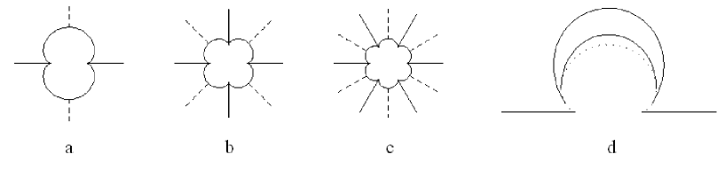
Figure 1: Equipotential lines $u=0$ (dashed lines), field lines $v=0$ and epicycloids for (a) $n=1$, (b) $n=2$ and (c) $n=3$. (d) The field lines end at the epicycloid (dotted line) (case $n=1$).

Those points of the $e$-plane lying on the circle $|e|=2b$ satisfy $(2b)/e=\overline{e}/(2b)$. So, if ${\it Im}[e\ dw/de]=0$ on the circle $|e|=2b$, then $dz$ vanishes. To satisfy this reality condition we will substitute the Coulombian seed,

$$e\ \frac{dw_{C}}{de}=-\frac{n\ A}{n+1}\ \left(\frac{e}{nA}\right)^{\frac{n}{n+1}}\ ,$$ (44)

with the improved seed

$$e\ \frac{dw}{de}=-\frac{n\ A}{n+1}\ \frac{\left(\frac{2b}{nA}\right)^{\frac{n}{n+1}}}{\left[\left(\frac{2b}{e}\right)^{\frac{\alpha\ n}{n+1}}+\left(\frac{e}{2b}\right)^{\frac{\alpha\ n}{n+1}}\right]^{1/\alpha}}\ .$$ (45)

For $\alpha>0$, this seed recovers the Coulombian form in the limit $b\rightarrow\infty$. Besides it is real on the circle $|e|=2b$ because it is $(2b)/e=\overline{e}/(2b)$ ($A$ is assumed to be positive). Let us show the behavior of the seed on the circle $|e|=2b$ by replacing $e=2b\ \exp[-i(n+1)\theta]$ in Eq. (45):

$$e\ \frac{dw}{de}\propto\frac{1}{\cos^{1/\alpha}[\alpha\,n\,\theta]}\ .$$ (46)

So the improved seed is divergent at $\alpha\,\theta_{k}=k\,\pi/(2n)$ ($k$ is odd) and $dz$ remains indeterminate there. Therefore, the curve where the field attain its upper bound limit $|e|=2b$ cannot be reduced to a point. The improved seed (45) just substitutes the singular epicycloid by curves (actually straight lines) where the maximal field possesses the discretized directions $(n+1)\theta_{k}$. Let us consider this result in the light of the simpler dipole case. For $n=1$, it is $\alpha\,\theta=\pm\pi/2$; so, if $\alpha=1$ is chosen, then the singular curve is reduced to a straight line where the field has direction $\pm\pi$. This means that the $n=1$ epicycloid has been reduced to the segment joining both cusps in Figure 1(a). In general, the choice $\alpha=1$ substitutes the singular epicycloid for a symmetric $2n$-vertexes polygonal closed curve whose sides coincide with the maximal field directions $(n+1)\theta_{k}$, ($k$ is odd). Thus, the vertexes become the only sources of field lines (point-like charges). In sum, except for the dipole case, the inner region is not removed. However, the fact that the curve separating the outer and inner regions now coincides with maximal field lines creates the proper conditions to continuously match the inner and outer solutions.

The integration of Eq. (43) with the seed (45) yields $z(e,\overline{e})$:

$$z= \left(\frac{nA}{2b}\right)^{\frac{1}{n+1}}\ \Bigg{[}\left(\frac{2b}{e}\right)^{\frac{1}{n+1}}F\left(-\frac{1}{2n},1;1-\frac{1}{2n};-\left(\frac{e}{2b}\right)^{\frac{2n}{n+1}}\right)-$$ (47)

$$-\frac{\left(\frac{\overline{e}}{2b}\right)^{\frac{2n+1}{n+1}}}{2n+1}\ F\left(1+\frac{1}{2n},1;2+\frac{1}{2n};-\left(\frac{\overline{e}}{2b}\right)^{\frac{2n}{n+1}}\right)\Bigg{]}\ ,$$

where $F(a,b,c;\xi)$ is the hypergeometric function. The expression (47) cannot be inverted to obtain the field $e(z,\overline{z})$, which is left in this implicit form. Remarkably, $F(a,b,c;\xi)$ $=$ $1+{\cal O}(\xi)$; then, the leading Born-Infeld correction comes from the first term in the bracket, being of order $b^{-\frac{2n}{n+1}}$. Instead, if the Coulombian seed were used then the Born-Infeld correction would come only from the second term in Eq. (26), so being of order $b^{-2}$ (see Eq. (40)). This difference is due to the presence of $b$ in the improved seed (45), as a consequence of a boundary condition ensuring the point-like character of the charges.

The Eq. (45) can be integrated to get the complex potential:

$$w(e)=-A\left(\frac{e}{nA}\right)^{\frac{n}{n+1}}\;F\left(\frac{1}{2},1;\frac{3}{2};-\left(\frac{e}{2b}\right)^{\frac{2n}{n+1}}\right)=-A\,\left(\frac{2b}{nA}\right)^{\frac{n}{n+1}}\ \arctan\left[\left(\frac{e}{2b}\right)^{\frac{n}{n+1}}\right]\ ,$$ (48)

or

$$\left(\frac{e(w)}{2b}\right)^{\frac{n}{n+1}}=\tan\left[-\left(\frac{nA}{2b}\right)^{\frac{n}{n+1}}\ \frac{w}{A}\right]\ .$$ (49)

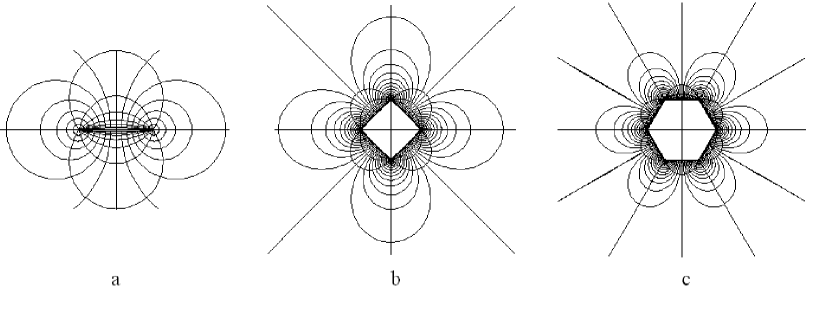
Figure 2: Equipotential and field lines for Born-Infeld $2^{n}$-pole configurations: (a) $n=1$, (b) $n=2$, (c) $n=3$.

By substituting this function in the Eq. (47) we obtain $z=z(w,\overline{w})$. By fixing ${\it Im}[w]=v_{o}$ we obtain the field lines $z(u,v_{o})$ as curves parametrized by the potential $u$ and labeled by $v_{o}$. Figure 2 shows the field lines for the cases $n=1,2,3$. In the case $n=1$, the maximum field is attained at the segment joining the two opposite charges. In the rest of the cases the maximum field lines form regular polygons which display charges of alternate signs in their $2n$ vertexes. On the sides of these polygons the field is $e_{k}=2b\ \exp[-i(n+1)\theta_{k}]=2b\ \exp[-i(n+1)k\pi/(2n)]$, $k$ is odd ($|k|\leq 2n-1$). By replacing this field in the complex potential (48), we get $v=\pm\infty$ on the polygon. The sizes of the polygons are obtained by replacing $e=2b$ in Eq. (47). The hypergeometric function $F(a,b,c;\xi)$ is multivaluated; its principal branch has a cut on the real axis for $1\leq\xi<\infty$. When evaluated at $e=2b$, Eq. (47) gives the position of the charge lying on the positive $x$-semiaxis:

$$z|_{e=2b}=\left(\frac{nA}{2b}\right)^{\frac{1}{n+1}}\ \frac{\pi}{2n\ \sin[\frac{\pi}{2n}]}\ .$$ (50)

On this charge the potential $u$ reaches the bound value

$$u_{b}=-A\,\left(\frac{2b}{nA}\right)^{\frac{n}{n+1}}\frac{\pi}{4}\ .$$ (51)

At infinity the complex potential $w$ goes to zero.

VI The multipolar inner solutions

In order to complete the multipolar solutions $n>1$, we should fill the interior of the polygons with a field that continuously matches the outer field on the polygon boundary. So, we should start by choosing an inner seed preserving the symmetry of the configuration. Let us try the complex potential $w=-B\ z^{n}$, $B>0$, which possesses the same symmetries that the Coulombian outer potential. Then $e=dw/dz=-Bn\ z^{n-1}$, and so it is $w=-B(-e/nB)^{n/(n-1)}$. Notice that the potential and the field are negative on the positive $x$-semiaxis, as it should be expected to properly match with the outer solution. Therefore

$$e\ \frac{dw}{de}=-\frac{nB}{n-1}\ \left(\exp{[i\pi]}\ \frac{e}{nB}\right)^{\frac{n}{n-1}}\ .$$ (52)

We will improve this expression by changing it for

$$e\ \frac{dw}{de}=-\frac{nB}{n-1}\ \frac{\left(\frac{2b}{nB}\right)^{\frac{n}{n-1}}}{\left(\exp{[-i\pi]}\ \frac{2b}{e}\right)^{\frac{n}{n-1}}+\left(\exp{[i\pi]}\ \frac{e}{2b}\right)^{\frac{n}{n-1}}}\ .$$ (53)

The inner seed (53) is real on the circle $e=2b\ \exp[-i\theta(n-1)-i\pi]$, and indeterminate for $\theta_{k}=k\pi/(2n)$ ($k$ odd). The integration of Eq. (26) can be linked to the outer solution by changing $n\rightarrow-n$ and $e\rightarrow\exp{[i\pi]}\,e$. Then,

$$z= \left(\frac{2b}{nB}\right)^{\frac{1}{n-1}}\Bigg{[}\left(\frac{e}{2b}\,\exp{[i\pi]}\right)^{\frac{1}{n-1}}F\left(\frac{1}{2n},1;1+\frac{1}{2n};-\left(\frac{e}{2b}\,\exp{[i\pi]}\right)^{\frac{2n}{n-1}}\right)+$$ (54)

$$+\frac{\left(\frac{\overline{e}}{2b}\,\exp{[-i\pi]}\right)^{\frac{2n-1}{n-1}}}{2n-1}\ F\left(1-\frac{1}{2n},1;2-\frac{1}{2n};-\left(\frac{\overline{e}}{2b}\,\exp{[-i\pi]}\right)^{\frac{2n}{n-1}}\right)\Bigg{]}\ .$$

The complex potential $w(e)$ is

$$w(e)=-B\,\left(\frac{2b}{nB}\right)^{\frac{n}{n-1}}\ \arctan\left[\left(\frac{e}{2b}\,\exp{[i\pi]}\right)^{\frac{n}{n-1}}\right]\ .$$ (55)

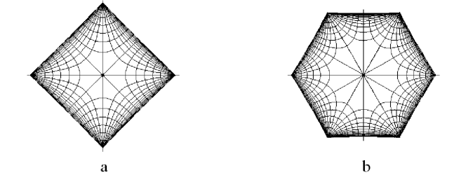
Figure 3: Born-Infeld $2^{n}$-pole configurations (inner solution): (a) $n=2$, (b) $n=3$.

The field lines $z(u,v_{o})$ can be obtained by replacing $e(w(u,v_{o}))$ in the Eq. (54). Figure 3 shows the inner field lines for the cases $n=2$ and $n=3$. To properly join this inner solution with the outer solution, we will match the positions of the charges by equalizing the points where the field is maximum. For this purpose, it will be enough to consider the solution on the positive $x$-semiaxis. There the field $e$ is real; it varies from $0$ to $-2b$, when going from the center to the vertex, and it varies from $2b$ to $0$ when going from the vertex to infinity. It is worth noticing that the evaluation of the bracket in Eq. (47) at $e=2b$ gives the same value that the evaluation of the bracket in Eq. (54) at $e=-2b$. Therefore, the inner and the outer solutions match if

$$\left(\frac{2b}{nB}\right)^{\frac{1}{n-1}}=\left(\frac{nA}{2b}\right)^{\frac{1}{n+1}}\ .$$ (56)

This relation also guarantees the continuity of the potential along the polygonal curve (cf. Eqs. (48) and (55)). Of course, the field $E$ is continuous too. In fact, the improved seeds (45) –with $\alpha=1$– and (53) have the ability of reducing the singular $e=2b$ curves to polygonal curves whose sides coincide with maximal field lines. This allows the continuity of $E$ both in direction and magnitude, whenever the Eq. (56) assures that the sizes of the inner and outer field structures fit each other. On the other hand, $D$ diverges on the $e=2b$ polygonal curve. This means that the vertexes cannot be regarded as isolated monopoles, although they are the sources of all the field lines. Actually they are strongly tied in a whole multipolar structure: as shown in Section 8, the divergence of $D$ entails an infinite force on each charge (cf. Eq. (63) with the divergent result (67)).

VII The dipole

We will rework the dipole case ($n=1$). Following the Eq. (49), the function $e(w)$ is

$$e=2b\ \tan^{2}\left[-\frac{w}{\sqrt{2bA}}\right].$$ (57)

We replace it in Eq. (25) to obtain $z=z(w,\overline{w})$ as

$$z=-\sqrt{\frac{A}{2b}}\ \left(\cot\left[\frac{w}{\sqrt{2bA}}\right]+\frac{w}{\sqrt{2bA}}-\tan\left[\frac{\overline{w}}{\sqrt{2bA}}\right]+\frac{\overline{w}}{\sqrt{2bA}}\right)\ .$$ (58)

Notice that $w/\sqrt{2bA}=\pm\,\pi/4$ implies that $e=2b$; then the charges are located at

$$z|_{e=2b}=\pm\ \sqrt{\frac{A}{2b}}\ \ \frac{\pi}{2}\ .$$ (59)

On the segment between the charges, the potential $u/\sqrt{2bA}$ varies in the range $[-\pi/4,\pi/4]$, while $v=\pm\infty$. On the rest of the $x$-axis it is $v=0$. One can easily verify that the equipotential curves $z=z(u_{o},v)$ are the circles

$$\left|\ z+\frac{u_{o}}{b}+\sqrt{\frac{A}{2b}}\ \cot\left[\frac{2\,u_{o}}{\sqrt{2bA}}\right]\right|^{2}=\frac{A}{2b}\ \cot^{2}\left[\frac{2\,u_{o}}{\sqrt{2bA}}\right]\ .$$ (60)

This is the solution studied in Section XI of Ref. Pryce1 .

The function $z=z(e,\overline{e})$ is obtained by substituting the potential $w(e)$ in the Eq. (58):

$$z=\sqrt{\frac{A}{2b}}\ \left(\left(\frac{e}{2b}\right)^{-\frac{1}{2}}+\arctan\left[\left(\frac{e}{2b}\right)^{\frac{1}{2}}\right]-\overline{\left(\frac{e}{2b}\right)^{\frac{1}{2}}}+\arctan\left[\overline{\left(\frac{e}{2b}\right)^{\frac{1}{2}}}\right]\right)\ .$$ (61)

If the field $e$ does a closed path around the origin in the $e$-plane, then $z\rightarrow-z$; so, a double turn around the origin in the $e$-plane completes a turn around the dipole in the $z$-plane. However, just one trip rounding the origin, but passing $e=-2b$, corresponds to a complete trip around a charge in the $z$-plane (passing by $e=-2b$ means crossing over the segment between the charges). The surrounded charge is infinite, since $-\infty<v<\infty$ (see Eq. (29)). This conclusion is also valid for the other multipoles.

VIII Electrostatic force

The force $\mathbf{P}$ on the charges inside a region is the flux of the stress tensor on the boundary of the region. In 2 dimensions, it is

$$P^{i}=-\oint_{\Gamma}\ T^{\,i\,j}\ n_{j}\ d\ell\ ,$$ (62)

where the normal vector $n_{x}\,d\ell=dy$, $n_{y}\,d\ell=-dx$ is exterior for a counterclockwise oriented path $\Gamma$ surrounding the charges (the flux is zero whenever no charges are surrounded). According to Eq. (7), it is

$$P\equiv P_{x}-i\,P_{y}=\frac{1}{4\pi}\oint_{\Gamma}\left[E(D_{x}\,dy-D_{y}\,dx\,)-i\,b^{2}(dx-i\,dy)\left(1-\sqrt{1-\frac{|E|^{2}}{b^{2}}}\right)\right]\ .$$ (63)

We will use Eqs. (19, 21) to replace $D_{x}\,dy-D_{y}\,dx$, and Eq. (25) to substitute $dx-i\,dy$; thus

$$P=\frac{1}{4\pi}\oint\left[E\ \frac{dw-d\overline{w}}{2\,i}-i\,b^{2}\left(\frac{d\overline{w}}{\overline{e}}+\frac{e}{4b^{2}}\,dw\right)\left(1-\sqrt{1-\frac{|E|^{2}}{b^{2}}}\right)\right]\ .$$ (64)

We can use Eq. (24) to replace $E$. In particular, it is

$$1-\sqrt{1-\frac{|\mathbf{E}|^{2}}{b^{2}}}=\frac{1}{2b^{2}}\ \frac{|e|^{2}}{1+\frac{|e|^{2}}{4\,b^{2}}}\ .$$ (65)

Then, Eq. (64) reduces to

$$P=-\frac{i}{8\pi}\ \oint\ e\ dw\ .$$ (66)

To compute the force (66) between the dipole charges, one can surround a charge by choosing $\Gamma$ as the closed path in the $z$-plane formed by the $y$-axis and a semi-circle at infinity. The field is Coulombian on the semi-circle at infinity: $|e|\sim r^{-2}$ and $|w|\sim r^{-1}$; thus, the flux at infinity vanishes. So, the force will come from the flux on the $y$-axis, where $u=0$, and $0<|v|<\infty$. By using the Eq. (57), the force (66) is written as the integral

$$P=-\frac{i}{4\pi}\ \int\limits_{-\infty}^{0}\ 2b\ \tan^{2}\left[-\frac{i\,v}{\sqrt{2bA}}\right]\ d(i\,v)=-\frac{b}{2\pi}\int\limits_{-\infty}^{0}\tanh^{2}\left[\frac{\,v}{\sqrt{2bA}}\right]\ dv\ ,$$ (67)

which diverges.

IX Electrostatic energy

The energy density $T^{00}$ of a Born-Infeld electrostatic field is (see Eq. (7))

$$T^{00}=\frac{1}{4\pi}\,\ \mathbf{E\cdot D}-\frac{b^{2}}{4\pi}\ \left(1-\sqrt{1-\frac{|\mathbf{E}|^{2}}{b^{2}}}\right)\ .$$ (68)

Born and Infeld succeeded in getting a finite self-energy for the three dimensional point-like charge because the first term in Eq. (68) diverges at the origin in a softer way than in Maxwell’s theory. This is the benefic effect of the regular behavior of $\mathbf{E}$ at the origin, even though the monopolar field $\mathbf{D}$ keeps its Coulombian form as mentioned in Section 2. This successful performance at the level of a monopole could break down for other multipoles, because the Coulombian divergence of $\mathbf{D}$ at the origin becomes more dramatic. However, the solutions obtained in Sections 3 and 4 show that Born-Infeld electrostatics spreads the multipolar sources in a set of individual charges on a polygonal curve. So, there is a hope that self-energies remain finite even for multipolar configurations. In terms of $e$, the electrostatic energy density (68) is

$$T^{00}=\frac{1}{4\pi}\,\left[\frac{|e|^{2}}{1-\frac{|e|^{4}}{16\,b^{4}}}-\frac{1}{2}\frac{|e|^{2}}{1+\frac{|e|^{2}}{4\,b^{2}}}\right]\ =\ \frac{\frac{|e|^{2}}{8\,\pi}}{1-\frac{|e|^{2}}{4b^{2}}}\ .$$ (69)

On the other hand, the volume is

$$dx\wedge dy=\frac{dz+d\overline{z}}{2}\ \wedge\ \frac{dz-d\overline{z}}{2\,i}\ =\ \frac{i}{2}\ dz\wedge d\overline{z}\ .$$ (70)

We will integrate the energy density (69) in the $z$-plane to obtain the electrostatic energy. We can also change the integration to the $w$-plane by using the Eq. (25):

$$dz\wedge d\overline{z}=\left(\frac{dw}{e}+\frac{\overline{e}}{4b^{2}}\,d\overline{w}\right)\wedge\left(\frac{d\overline{w}}{\overline{e}}+\frac{e}{4b^{2}}\,dw\right)=\frac{1}{|e|^{2}}\,\left(1-\frac{|e|^{4}}{16\,b^{4}}\right)\,dw\wedge d\overline{w}\ .$$ (71)

Therefore

$$T^{00}\ dx\wedge dy=\frac{i}{16\,\pi}\ \left(1+\frac{|e|^{2}}{4\,b^{2}}\right)\ dw\wedge d\overline{w}\ ,$$ (72)

where $(i/2)\,dw\wedge d\overline{w}$ is the volume in the $w$-plane.

We will work out the integration of the density (72) for the dipole configuration. Using the Eq.(57), it is

$$T^{00}\ dx\wedge dy=\frac{i}{16\,\pi}\ \left(1+\left|\tan\left[-\frac{w}{\sqrt{2bA}}\right]\right|^{4}\right)dw\wedge d\overline{w}\ ,$$ (73)

where $(i/2)\,dw\wedge d\overline{w}=du\,dv$. In the semi-plane $x<0$, it is $0<u<\sqrt{2bA}\pi/4$, $-\infty<v<\infty$. Then, the dipole electrostatic energy is

$$U=\int\ T^{00}\ dx\wedge dy=\frac{Ab}{2\,\pi}\ \int_{-\infty}^{\infty}dv\ \int_{0}^{\pi/4}du\ \left(1+\left|\tan\left[u+i\ v\right]\right|^{4}\right)\ .$$ (74)

The integral on the variable $v$ is divergent.

X Two opposite isolated charges

Let us now consider the Coulombian ingredients for the field of two equal but opposite charges $\lambda$, $-\lambda$ separated by a distance $d$:

$$w_{C}=\lambda\ {\rm Log}\left[\frac{z-\frac{d}{2}}{z+\frac{d}{2}}\right]\ .$$ (75)

Then

$$e_{C}=\frac{dw_{C}}{dz}=\frac{\lambda\ d}{z^{2}-\left(\frac{d}{2}\right)^{2}}\ ,$$ (76)

$$e\ \frac{dw_{C}}{de}=-\frac{\lambda\ \sqrt{e}}{\sqrt{e+\frac{4\lambda}{d}}}=-\frac{\sqrt{\lambda\ d}}{2\ \sqrt{\frac{d}{4\lambda}+\frac{1}{e}}}\ .$$ (77)

This last expression should be substituted by an improved seed accomplishing the reality condition. Additionally, one should require that the dipole field be recovered for $d\rightarrow 0$, $\lambda\rightarrow\infty$ (but $\lambda d$ remaining a constant). Even so, the answer seems not to be unique (see, however, Ref. Pryce2 and the comments included in footnote 6 and Section 11). We choose

$$e\ \frac{dw}{de}=-\ \frac{\sqrt{\frac{b\,\lambda\,d}{2}}}{\sqrt{\frac{bd}{2\lambda}+\left(\sqrt{\frac{2b}{e}}+\sqrt{\frac{e}{2b}}\right)^{2}}}\ ,$$ (78)

which has the right Coulombian limit, it goes to the Born-Infeld dipole for $d\rightarrow 0$ and $\lambda\rightarrow\infty$ (but $A=\lambda d$), and it is real on the circle $|e|=2b$. By expanding the binomial one gets

$$e\ \frac{dw}{de}=-\frac{\sqrt{\frac{b\,\lambda\,d}{2}}}{\sqrt{\frac{bd}{2\lambda}+2+\frac{2b}{e}+\frac{e}{2b}}}\ ,$$ (79)

which is the case studied in Section IX (example 3) of Ref. Pryce1 . For $d\rightarrow\infty$, one recovers the isotropic monopolar expression $e\,dw/de=-\lambda$ at every point where $e\neq 0$ (see Section 4). Instead, for finite values of $d$, $e\,dw/de$ is not isotropic in the $e$-plane even at the circle $e=2b\,\exp[i\vartheta]$ –i.e., at the charges–, where the radicand becomes $bd/(2\lambda)+2\,(1+\cos\vartheta)$. This is a characteristic feature of Born-Infeld solutions. On the contrary, the Coulombian field diverges at the charges; thus, the Coulombian expression (77) becomes monopolar-like at the charges. As it will be explained in the Conclusions, this non-isotropic behavior leads to the single-valuedness of the Born-Infeld field $e(z,\overline{z})$.

Let us review the benefits of passing from the Coulombian seed (77) to the improved seed (79) from a different point of view. One of the consequences is the splitting of the singularity at $e=-4\lambda/d$ in the Coulombian seed into two singularities $e_{1,2}$ on the negative real axis of the $e$-plane:

$$\frac{e_{1,2}}{2b}=-a\pm\sqrt{a^{2}-1}\,,\qquad a\equiv 1+\frac{bd}{4\lambda}\,.$$ (80)

Notice that it is $|e_{1}|<2b$ and $|e_{2}|>2b$: $e_{1}$ and $e_{2}$ are respectively inside and outside the circle $|e|=2b$. Actually $e_{1}$ is the value of $e$ at the center of the configuration. In fact, the symmetry of the configuration implies that $e$ is real and negative only on the $y$-axis and the segment between the charges. Besides, on the $y$-axis it is $u=0$ (like in the Coulombian case), while on the segment between the charges it is $v=$constant. So, for $e<0$, $dw$ passes from being imaginary to becoming real at $z=0$. This change of behavior happens when the radicand in the Eq. (79) changes sign, i.e. at $e=e_{1}$. So, $e_{1}$ is the value of $e$ at $z=0$ (if $b\rightarrow\infty$, then $e_{1}$ goes to the Coulombian value $-4\lambda/d$). The improved function (79),

$$e\ \frac{dw}{de}=-b\,\sqrt{\lambda\,d}\ \frac{\sqrt{e}}{\sqrt{(e-e_{1})\,(e-e_{2})}}\ ,$$ (81)

is multivalued; it has a branch cut inside the circle $|e|=2b$ between $e_{1}$ and $0$ (it has also a branch cut outside the circle between $e_{2}$ and $\infty$). This cut means that there are two different ways of surrounding $e=0$ inside the circle. If the path crosses the cut (i.e., if the path is close to $e=0$), then the function (79) will return to its initial value after two turns. This behavior is typical of a dipolar structure: far from the charges, where the field is near to zero, a path in the $z$-plane closes after two complete turns of the field; this feature is reflected by the function (81) which is directly related to the position via the Eq. (26). However, if the sources are constrained to be just isolated charges, it should be possible to surround an individual charge and find a structure similar to a monopole (no branch cuts in such case). This is the reason why the branch cut cannot reach the circle $|e|=2b$: since $2b$ is the upper bound for $|e|$, which is attained at the charge positions, then there must exist closed paths in the $e$-plane near (but inside) the circle $|e|=2b$ that do not cross any branch cut of the seed $e\,dw/de$. On the contrary, the dipole displays a branch cut that extends from $-2b$ to $0$; in such case, the only way of surrounding an individual charge is passing the $e=-2b$ point (i.e., crossing the dipole singular segment). In both cases –two opposite separated charges and dipole– the multivalued function $e\,dw/de$ has two Riemann sheets in the domain $|e|\leq 2b$, which correspond to each surroundable charge. Figure 4(a,b) shows the $e$-plane for two opposite separated charges and the dipole, respectively; it also includes a path surrounding an individual charge. We conclude that any physically meaningful Born-Infeld configuration generated by isolated charges must allow for closed paths near the circle $|e|=2b$ which do not cross any branch cut of the seed $e\,dw/de$. Nevertheless, some branch cuts inside the circle are needed to open a Riemann sheet for each individual charge. Since the functions of the form $e^{m}\,dw/de$ are well behaved in a ring including the circle $|e|=2b$, then Cauchy-Goursat theorem states that their integrals on closed paths that goes near the circle $|e|=2b$ (without crossing branch cuts) are independent of the path. So, this kind of integrals can be performed directly on the circle. As an application, let us compute the individual charges in the Born-Infeld field of two opposite separated charges. We use Eq. (29)

$$2\pi\,i\ Q=\oint_{\Gamma}dw=\oint_{\Gamma}\frac{dw}{de}\ de\ ,$$ (82)

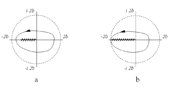
Figure 4: Branch cuts of the multivalued function $e\,dw/de$: (a) two equal but opposite charges; (b) dipole.

where $\Gamma$ is a counterclockwise path surrounding the charge in the $z$-plane. In the $e$-plane, it corresponds to a closed path near the circle; so we will integrate on the circle: $e=2b\exp[i\vartheta]$. According to the Eq. (79), it is

$$2\pi\,i\ Q=\pm\sqrt{\frac{b\lambda\ d}{2}}\int_{0}^{2\pi}\frac{i\ d\vartheta}{\sqrt{2(a+\cos{\vartheta})}}\ .$$ (83)

So, the value of $Q$ is

$$Q=\pm\frac{\lambda}{\pi}\sqrt{a-1}\ \left[\frac{K\left(\sqrt{\frac{-2}{a-1}}\right)}{\sqrt{a-1}}+\frac{K\left(\sqrt{\frac{2}{a+1}}\right)}{\sqrt{a+1}}\right]\ ,$$ (84)

where $K(k)$ is the complete elliptic integral of the first kind (here we follow the notation of Refs. Abra ; Grad ). $|Q|$ ranges from $0$, for $a\rightarrow 1_{+}$, to $\lambda$ for $a\rightarrow\infty$. Therefore, the individual charges are smaller than those suggested by the far (Coulombian) field.

We can also compute the force (66) on an individual charge by integrating on the circle $e=2b\,\exp[i\,\vartheta]$. Then, we use Eq. (79) to write the force as

$$P=\mp\frac{i}{8\pi}\oint\,e\,\frac{dw}{de}\ de=\pm\frac{i\,\lambda}{8\pi}\sqrt{2(a-1)}\int_{0}^{2\pi}\frac{2b\,i\,exp[i\,\vartheta]}{\sqrt{2(a+\cos[\vartheta])}}\ d\vartheta\ .$$ (85)

Therefore,

$$P=\mp\frac{\lambda\,b\,\sqrt{a-1}}{4\,\pi}\ \left[-\frac{2\,K\left(\sqrt{\frac{-2}{a-1}}\right)}{\sqrt{a-1}}+\frac{2\,K\left(\sqrt{\frac{2}{a+1}}\right)}{\sqrt{a+1}}+\frac{\pi\,F\left(\frac{1}{2},\frac{3}{2},2;\frac{-2}{a-1}\right)}{\sqrt{a-1}}-\frac{\pi\,F\left(\frac{1}{2},\frac{3}{2},2;\frac{2}{a+1}\right)}{\sqrt{a+1}}\right].$$ (86)

This expression goes to $\pm\lambda^{2}/(2d)$ when $a\rightarrow\infty$ (Coulombian limit). But it vanishes when $a$ goes to $1_{+}$ (i.e., when the charges approach each other). This result is consistent with the vanishing of the charges when they go together. The force reaches its maximum value at $a=1.15746$, i.e. at $d=0.63\,\lambda/b$. It is always lower than the Coulombian force; at the leading order in $b^{-1}$ it is

$$P=\pm\,\frac{\lambda^{2}}{2\,d}\,\left(1-\frac{6\,\lambda}{b\,d}\right)+{\cal O}(b^{-2})\ .$$ (87)

However, except for the Coulombian limit, $d$ does not coincide with the real distance between the charges. The distance should be computed by integrating the Eq. (26). The field $e$ on the $x$-axis is real and varies from $e_{1}$ at $x=0$ to $-2b$ at the position $x_{L}$ of the left charge. Then

$$x_{L}=\int_{e_{1}}^{-2b}\left[\frac{1}{e}\,\frac{dw}{de}+\frac{e}{4b^{2}}\,\frac{dw}{de}\right]\,de=-\frac{\lambda}{2b}\,\sqrt{2(a-1)}\,\int_{\frac{e_{1}}{2b}}^{-1}\frac{1+\varepsilon^{-2}}{\sqrt{2a+\varepsilon^{-1}+\varepsilon}}\ d\varepsilon\,,$$ (88)

where $e_{1}/(2b)=-a+\sqrt{a^{2}-1}$ (see Eq. (80)). This is an involved integral. Nevertheless, it can be verified that $x_{L}\rightarrow 0$ if $d\rightarrow 0$, and $x_{L}\rightarrow-d/2$ in the Coulombian limit.

XI Conclusions

We have displayed a method to obtain Born-Infeld electrostatic solutions in 2 dimensions, which is condensed in the paragraph after the Eq. (25). This procedure is a cleaner version of the one developed by Pryce in Section II of Ref. Pryce1 . The method starts from a holomorphic (except at some isolated points) seed $w(e)$, where $w$ is the complex potential and $e$ is a complex variable linked to the electric field $E$, to then obtain a non-holomorphic function $z(e,\overline{e})$ connecting the field with the Cartesian coordinates $z=x+i\,y$. Although any seed $w(e)$ could be employed, one should prescribe that $w(e)$ goes to the Coulombian potential $w_{C}(e)$ for $b\rightarrow\infty$, in order to reobtain the Coulombian field in the weak field region. Moreover, $e\,dw/de$ has to be real on the circle $|e|=2b$ in order that the field sources correspond just to isolated points. The way of achieving this reality condition conferred interesting symmetries to the seed $w(e)$ and the resulting function $z(e,\overline{e})$. In fact we have chosen seeds $w(e)$ such that $e\,dw/de$ does not change under the transformation $e/(2b)\rightarrow 2b/e$ (see Eqs. (45), (53) and (79)). On the circle $|e|=2b$, $e/(2b)$ and $2b/e$ are complex conjugate. So $e\,dw/de$ is real on the circle, which is the requirement to get isolated singularities. Therefore,

$$e\ \frac{dw}{de}=\frac{e}{2b}\,\frac{dw(\frac{e}{2b})}{d(\frac{e}{2b})}=\frac{2b}{e}\ \frac{dw(\frac{2b}{e})}{d(\frac{2b}{e})}=\frac{1}{e}\ \frac{dw(\frac{2b}{e})}{d(\frac{1}{e})}=-e\ \frac{dw(\frac{2b}{e})}{de}\,,$$ (89)

that it can be integrated to obtain

$$w\left(\frac{e}{2b}\right)=-w\left(\frac{2b}{e}\right)+constant.$$ (90)

The complex potentials (48) and (55) effectively possess this property since

$$\arctan[\xi]=-\arctan\left[\frac{1}{\xi}\right]+\frac{\pi}{2}\ ,\hskip 21.68121pt\xi\in\mathbb{C}.$$ (91)

On the other hand, the Coulombian monopolar potential (30) has already the property (90); so, it does not need any improvement. In Eq. (43), the symmetry in question implies that the function $z(e,\overline{e})$ has the form

$$z(e,\overline{e})=f\left(\frac{2b}{e}\right)-f\left(\frac{\overline{e}}{2b}\right)+constant.$$ (92)

where

$$f^{\prime}(\xi)=f^{\prime}\left(\frac{1}{\xi}\right).$$ (93)

Properties (92, 93) are evident in the monopolar solution (32). For the solutions (47) and (54), the properties are verified by means of the identity

$$\xi^{\frac{1}{n+1}}F\left(-\frac{1}{2n},1;1-\frac{1}{2n};-\frac{1}{\xi}\right)=\frac{\xi^{\frac{2n+1}{n+1}}}{2n+1}\,F\left(1+\frac{1}{2n},1;2+\frac{1}{2n};-\xi^{\frac{2n}{n+1}}\right)+\frac{\pi}{2n\,\sin[\frac{\pi}{2n}]}\ ,$$ (94)

where $-\pi<\arg[\xi]<\pi$.

It was also explained in Section 10 that the chosen seeds caused that those closed paths in the $e$-plane going near the circle $|e|=2b$ do not cross the branch cuts of functions $f^{\prime}$. As a consequence, those integrals surrounding individual charges can be performed directly on the circle (Cauchy-Goursat theorem). The functions $z(e,\overline{e})$ possessing all these characteristics guarantee the single-valuedness of the field $e(z,\overline{z})$. In fact, let us surround a charge and use the properties (92, 93):

$$\oint dz=\oint f^{\prime}\left(\frac{1}{\xi}\right)\,d\left(\frac{1}{\xi}\right)-\oint f^{\prime}(\overline{\xi})\,d\overline{\xi}\ ,$$ (95)

where $\xi=e/(2b)$. Both integrals in the right side are equal. In fact, since the integrands are well behaved near the circle, then the closed path can be deformed into the circle $\xi=\exp[i\,\vartheta]$, where the integrals become manifestly equal. Therefore it is $\oint dz=0$, i.e., closed paths in the $e$-plane are also closed paths in the $z$-plane, which means that the field is single-valued.

Finally, we have shown that the force between two equal but opposite charges $\pm\lambda$ reaches the maximum value at $d=0.63\,\lambda/b$, but then it decreases up to vanish when the charges approach each other ($d$, $\lambda$ are not the actual distance and charge, but their magnitudes inferred from the far (Coulombian) field). In the weak field region, the interaction force departs from its Coulombian partner at the first order in $b^{-1}$ (see Eq. (87)). As remarked in Section 5, the corrections of order lower than $2$ do not come from the Eq. (26), but originate in boundary conditions to guarantee the point-like character of the sources.

- (1) M. Born, Proc. R. Soc. (London) A 143 (1934), 410.
- (2) M. Born and L. Infeld, Nature 132 (1933), 1004.
- (3) M. Born and L. Infeld, Proc. R. Soc. (London) A 144 (1934), 425.
- (4) M. Born and L. Infeld, Proc. R. Soc. (London) A 147 (1934), 522.
- (5) E.S. Fradkin and A.A. Tseytlin, Phys. Lett. B 163 (1985), 123.
- (6) A. Abouelsaood, C. Callan, C. Nappi and S. Yost, Nucl. Phys. B 280 (1987), 599.
- (7) R.G. Leigh, Mod. Phys. Lett. A 4 (1989), 2767.
- (8) R.R. Metsaev, M.A. Rahmanov and A.A. Tseytlin, Phys. Lett. B 193 (1987), 207.
- (9) A.A. Tseytlin, Nuc. Phys. B 501 (1997), 41.
- (10) A.A. Tseytlin, in The many faces of the superworld, ed. M. Shifman, World Scientific, Singapore (2000).
- (11) J. Plebanski, Lectures on non linear electrodynamics, Nordita Lecture Notes, Copenhagen, 1968.
- (12) S. Deser and R. Puzalowski, J. Phys. A 13 (1980), 2501.
- (13) G. Boillat, J. Math. Phys. 11 (1970), 941.
- (14) M. Novello, V.A. De Lorenci, J.M. Salim and R. Klippert, Phys. Rev. D 61 (2000), 045001.
- (15) H. Salazar Ibarguen, A. García and J. Plebanski, J. Math. Phys. 30 (1989), 11.
- (16) B.M. Barbashov and N.A. Chernikov, Sov. Phys. JETP 24 (1967), 437.
- (17) R. Ferraro, Phys. Rev. Lett. 99 (2007), 230401.
- (18) M. Aiello, G.R. Bengochea and R. Ferraro, Phys. Lett. A 361 (2007), 9.
- (19) R. Ferraro, J. Phys. A: Math. Theor. 43 (2010), 195202.
- (20) G.W. Gibbons and C.A.R. Herdeiro, Phys. Rev. D 63 (2001), 064006.
- (21) M.H.L. Pryce, Proc. Cambr. Phil. Soc. 31 (1935), 50.
- (22) M.H.L. Pryce, Proc. Cambr. Phil. Soc. 31 (1935), 625.
- (23) R. Ferraro, Phys. Lett. A 325 (2004), 134.
- (24) R. Courant, Dirichlet’s principle, conformal mapping and minimal surfaces, Interscience Pub. Inc., New York (1950).
- (25) R. Ferraro and M.E. Lipchak, Phys. Rev. E 77 (2008), 046601.
- (26) M. Abramowitz and I.A. Stegun (eds.), Handbook of mathematical functions, Dover Publications, New York (1965).
- (27) I.S. Gradshteyn and I.M. Ryzhik, Table of integrals, series and products, Academic Press, New York (2007).