Predicted and Verified Deviation from Zipf’s Law in Growing Social Networks

Abstract

Zipf’s power law is a general empirical regularity found in many natural and social systems. A recently developed theory predicts that Zipf’s law corresponds to systems that are growing according to a maximally sustainable path in the presence of random proportional growth, stochastic birth and death processes. We report a detailed empirical analysis of a burgeoning network of social groups, in which all ingredients needed for Zipf’s law to apply are verifiable and verified. We estimate empirically the average growth $r$ and its standard deviation $\sigma$ as well as the death rate $h$ and predict without adjustable parameters the exponent $\mu$ of the power law distribution $P(s)$ of the group sizes $s$. The predicted value $\mu=0.75\pm 0.05$ is in excellent agreement with maximum likelihood estimations. According to theory, the deviation of $P(s)$ from Zipf’s law (i.e., $\mu<1$) constitutes a direct statistical quantitative signature of the overall non-stationary growth of the social universe.

Power law distributions,

$$p(s)\sim 1/s^{1+\mu}~{},$$ (1)

are ubiquitous characteristics of many natural and social systems. The function $p(s)$ is the density associated with the probability $P(s)={\rm Pr}\{S>s\}$ that the value $S$ of some stochastic variable, usually a size or frequency, is greater than $s$. Among power law distributions, Zipf’s law states that $\mu=1$, i.e., $P(s)\sim s^{-1}$ for large $s$. Zipf’s law has been reported for many systems Saichev et al. (2009), including word frequencies Zipf (1949), firm sizes Axtell (2001), city sizes Gabaix (1999), connections between Web pages Kong et al. (2008) and between open source software packages Maillart et al. (2008), Internet traffic characteristics Adamic and Huberman (2000), abundance of expressed genes in yeast, nematodes and human tissues Furusawa and Kaneko (2003) and so on. The apparent ubiquity and universality of Zipf’s law has triggered numerous efforts to explain its validity. Deviations from Zipf’s law provide also important informative insights in the dynamics of the corresponding systems.

Since H. Simon’s pioneering work Simon (1955, 1960); Ijri and Simon (1977), a crucial ingredient in the generating mechanism of Zipf’s law is understood to be Gibrat’s rule of proportional growth Gibrat (1931), more recently rediscovered under the name of “preferential attachment” in the context of networks Barabasi and Albert (1999). Expressed in continuous time in terms of the size $S(t)$ of a firm, a city or, more generally, a social group, Gibrat’s rule corresponds to the geometric Brownian motion

$$dS(t)=S(t)\left(r\,dt+\sigma\,dW(t)\right)~{},$$ (2)

where the stochastic growth rate $r+\sigma dW/dt$ is decomposed into its average $r$ and its fluctuation part with amplitude determined by the standard deviation $\sigma$, while $W(t)$ is a standard Wiener process. Gibrat’s rule alone cannot produce (1), since the solution of equation (2) has a log-normal distribution. Simon and many other authors invoked an addition ingredient, corresponding to various modifications of the multiplicative process when $S(t)$ becomes small. Then, under very general conditions, the distribution of $S$ becomes a power law, with an exponent $\mu$ that is a function of the distribution of the multiplicative factors Kesten (1973); Sornette (1998); Gabaix (2009).

The fact that the exponent $\mu$ is often found close to $1$ requires another crucial ingredient. One particularly intriguing proposition is that Zipf’s law corresponds to systems that are growing according to a maximally sustainable path Malevergne et al. (2010). In other words, when Zipf’s law holds, the set of stochastically growing entities $\{S_{i}(t),i=1,2,...,n,..\}$ is delicately poised at a dynamical critical growth point. Within a general framework in which (i) entities are born at random times, (ii) grow stochastically according to (2), and (iii) can disappear or die according to various stochastic processes with some hazard rate $h$, the explicit calculation of the exponent $\mu$ confirms the above optimal growth condition associated with Zipf’s law ($\mu=1$) Malevergne et al. (2010).

Here, we present an empirical test of the optimal growth condition for Zipf’s law by testing the formula for exponent $\mu$ (see below) on a unique database obtained from a Web platform of collaborative social projects (Amazee.com). In this dataset, we verify empirically that proportional growth holds, we measure the parameters $r,\sigma$, $h$ and the exponent $\mu_{\rm exp}$ of the power law distribution of project sizes. We show that the theory leading to the maximum sustainable growth principle explains remarkably well the empirical value $\mu_{\rm exp}$, with no adjustable parameters.

The theory is based on the following assumptions Saichev et al. (2009); Malevergne et al. (2010). Consider a population of social groups (firms, cities, projects, and so on), which can take different forms and can be applied in many different contexts.

1. There is a flow of group entries, i.e., a sequence of births of new groups. The times $\{t_{1}<t_{2}<...<t_{i}<...\}$ of entries of new groups follow a Poisson process with constant intensity (generalizations to a vast class of non-Poisson processes do not modify the key result Saichev et al. (2009); Malevergne et al. (2010)).

2. At time $t_{i}$, $i\in{\mathbb{N}}$, the initial size of the new entrant group $i$ is a random variable $s_{0,i}$. The sequence $\left\{s_{0,i}\right\}_{i\in{\cal N}}$ is the result of independent and identically distributed random draws from a common random variable $\tilde{s}_{0}$. All the draws are independent of the entry dates of the groups.

3. Gibrat’s rule of proportional growth holds. This means that, in the continuous time limit, the size $S_{i}(t)$ of the $i^{th}$ group at time $t\geq t_{i}$, conditional on its initial size $s_{0}^{i}$, is solution to the stochastic differential equation (2), where the drift $r$ and the volatility $\sigma$ are the same for all groups but the Wiener process $W_{i}(t)$ is specific to each project $i$.

4. Groups can exit (disappear) at random, with constant hazard rate $h\geq 0$, which is independent of the size and age of the group.

Under these conditions, the central result of Malevergne et al. (2010) reads as follows. Defining

$$\mu:=\frac{1}{2}\left[\left(1-2\cdot\frac{r}{\sigma^{2}}\right)+\sqrt{\left(1-2\cdot\frac{r}{\sigma^{2}}\right)^{2}+8\cdot\frac{h}{\sigma^{2}}}\right]~{},$$ (3)

provided that ${\rm E}\left[\tilde{s}_{0}^{\mu}\right]<\infty$, and for times larger than

$$t_{\rm transient}=\left[\left(r-\frac{\sigma^{2}}{2}\right)^{2}+2\sigma^{2}h\right]^{-1/2}~{},$$ (4)

the average distribution of project’s sizes follows an asymptotic power law with tail index $\mu$ given by (3), in the following sense: the average number of projects with size larger than $s$ is proportional to $s^{-\mu}$ as $s\to\infty$. As a corollary, the exponent $\mu$ of the distribution of sizes takes the value $1$ corresponding to Zipf’s law, if and only if $r=h$.

In order to understand the corollary, notice that $r-h$ represents the average growth rate of an incumbent group. Indeed, considering a group present at time $t$, during the next instant $dt$, it will either exit with probability $h\cdot dt$ (and therefore its size declines by a factor $-100\%$) or grow at an average rate equal to $r\cdot dt$, with probability $(1-h\cdot dt)$. The coefficient $r$ is therefore the conditional growth rate of projects, conditioned on not having died yet. Then, the unconditional expected growth rate over the small time increment $dt$ of an incumbent group is $(r-h)\cdot dt+O\left((dt^{2}\right)$. The statistically stationary regime, in the presence of a stationary population of group forming individuals, corresponds to condition $r=h$. Malevergne et al. Malevergne et al. (2010) showed that this condition can be easily generalized to the case where the population of group forming individuals grows itself with some exponential rate, as is the minimal viable group size Malevergne et al. (2010). Then, this condition translates into that for the maximum sustainable growth of the universe of groups, as mentioned above.

Our strategy is to find an empirical dataset in which (i) all ingredients of the theory can be verified explicitly, (ii) all parameters $r,\sigma$ and $h$ can be measured directly and (iii) the empirical distribution of group sizes can be compared with to prediction (1) with (3). We have found such a database, with Amazee.com, which is a Web-based platform of collaboration. Using Amazee’s Web-platform, anyone with an idea for a collaborative project can sign in and use the website to gather followers, who will together help the project owner to accomplish the project. An Amazee project can be of any type of activities, such as arts and culture, environment and nature, politics and beliefs, science and innovation, social and philanthropic, sports and leisure, and so on. Most of the projects are public, for instance, “build a strong community of Internet entrepreneurs in Switzerland to exchange information and have fun” (Web Monday Zurich), “connect all women working in the Swiss ICT industry” (Tech Girls Switzerland), “to provide fresh running water to each home in the small African village of Dixie” (Water for Dixie), and so on. Amazee.com provides a set of features covering the entire lifetime of a typical project, such as project planning, participants recruiting, fund raising, events and meetings hosting, communication, files archiving, and so on. Users join Amazee.com by either creating a new project, or participating in projects created by others. The Amazee data we analyze contains the complete recording in time of the activities of all users creating and joining all the projects in existence from February 2008 till May 2010.

Projects can be seen as proxies of many naturally occurring entities, such as social groups, firms, cities, investment vehicles, and so on, each driven by some goal, competition, and interaction within social networks. The detailed knowledge of the activity of the participants of all projects provides a remarkable opportunity to dissect and understand the dynamics of such systems. In the present study, we restrict our attention to the simplest measure of size, namely the number $S_{i}$ of members of project $i$.

Table 1: Descriptive statistics of the sizes of Amazee’s projects at different times, showing that most projects have a size of just a few individuals while a few projects have hundreds to more than one thousand members. Dates are in format day/month/year.

	07.08.2008	08.02.2009	07.08.2009	08.05.2010
Number of projects	436	1165	1562	1829
Mean size	5	10	9	8
Minimum size	1	1	1	1
Maximum size	83	1110	1114	1120
Median size	2	2	2	1

Amazee’s platform started on February, 2008. We analyze four snapshots of the database, on 7 August 2008, on 8 February 2009, on 7 August 2009 and on 8 March 2010. The first snapshot is six months after the birth of the operations on Amazee.com. With the parameter values for $r,\sigma$ and $h$ determined below, formula (4) predicts a transient of 50-400 days. Therefore, except for the first snapshot, we should observe a reasonable convergence to the expected power law distribution.

Table 1 and Fig 1 confirm that the distributions of project sizes obtained for these four snapshots are power laws (1) ($p>0.05$ of a Kolmogorov-Smirnov (K-S) test for the three last snapshots), with some significant deviation only for the earliest snapshot. This deviation can be interpreted as only a partial convergence to the stationary growth regime, confirmed by the much smaller maximum size observed in the first snapshot. K-S tests on the same data for goodness of fit using competing distributions such as the exponential distribution and the log normal distribution yield $p$-values less than $0.01$, confirming the power law as the best model.

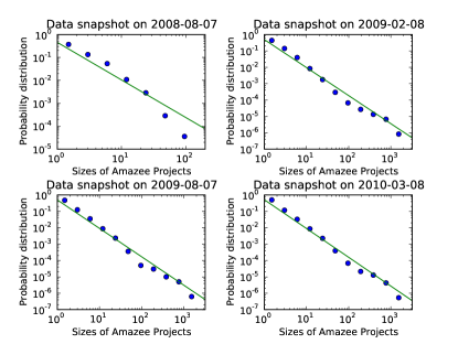
Figure 1: Blue dots: Probability distributions of Amazee project sizes measured for four snapshots on 7 August 2008, on 8 February 2009, on 7 August 2009 and on 8 March 2010. The maximum likelihood fits are shown by the green lines, with exponents $\mu$ respectively equal to $0.64$, $0.71$, $0.74$, $0.76$.

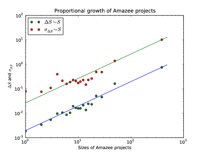
Figure 2: Test of Gibrat’s law for the proportional growth of Amazee project sizes until 8 March 2010. The slopes of the fitted straight lines are exactly $1$.

Because the numbers of project members are integers, the exponents $\mu$ corresponding to the empirical distributions shown in Fig 1 are estimated using the maximum likelihood method (ML) with the normalized discrete version of (1), $p(s)=\frac{s^{-(1+\mu)}}{\zeta(1+\mu)}$, where $\zeta(x)$ is the Riemann zeta function: $\zeta(x)=\sum_{s=1}^{\infty}s^{-x}$. The exponents are found around $0.7$, with confidence intervals clearly excluding $1$. We check the robustness of this conclusion by estimating the exponents $\mu$ for the four snapshots as a function of a lower threshold above which the MLE is performed. For the three last snapshots, we find stable estimations, with the $95\%$ confidence intervals excluding the value $1$. We can thus conclude that Zipf’s law is rejected for this dataset.

Table 2: For each of the four snapshots of the amazee database, we report the parameters $r,\sigma$ and $h$ as explained in the text. Reporting these parameters in expression (3) yields the predicted exponents $\mu$, which is compared with the empirical exponents $\mu$ estimated by maximum likelihood (MLE). For each cell value, the 95% confidence interval is obtained by bootstrapping over 10’000 realizations. Dates are in format day/month/year.

Date	07.08.2008	08.02.2009	07.08.2009	08.03.2010
$r$	0.11 [0.074, 0.20]	0.031 [0.027, 0.036]	0.027 [0.024, 0.031]	0.019 [0.017, 0.021]
$\sigma$	0.30 [0.23, 0.41]	0.18 [0.16, 0.20]	0.18 [0.16, 0.20]	0.19 [0.15, 0.24]
$h$	0.096 [0.065, 0.17]	0.021 [0.019, 0.025]	0.017 [0.015, 0.019]	0.011 [0.0099, 0.012]
$\mu$ (MLE)	0.64 [0.58, 0.70]	0.71 [0.67, 0.76]	0.73 [0.69, 0.78]	0.76 [0.72, 0.80]
$\mu$ (TH))	0.89 [0.78, 1.05]	0.78 [0.74, 0.81]	0.73 [0.70, 0.75]	0.75 [0.71, 0.79]

We now test formula (3). For this, we test if model (2) holds and proceed to estimating the parameters $r,\sigma$ and $h$. The proportional growth model posits that, for sufficiently small time intervals $\Delta t$, the mean ${\rm E}[\Delta S]$ and the standard deviation $\sigma_{\Delta S}$ of the increment of the size $S$ of a given project should both be proportional to $S$. To test this proposition, all the Amazee projects are pooled together in 100 size intervals over all four snapshots. For each of the 100 size intervals, Figure 2 plots the average daily increase of project sizes (${\rm E}[\Delta S]$) and its standard deviation $\sigma_{\Delta S}$ as a function of $S$. Linear regressions give very high $R^{2}$’s, larger than $0.995$, confirming that Gibrat’s law holds. The parameters $r$ and $\sigma$ are estimated as the mean and standard deviations of the set of daily growth rates, and are reported in Table 2. Note that $\sigma_{\Delta S}$ is much larger than $\Delta S$, i.e., the stochastic component of the proportional growth clearly dominates (an essential condition for a power law to emerge in the model Saichev et al. (2009)).

Next, we find that the rate of birth of new projects on amazee.com is approximately described by a Poisson process, such that the probability that $n$ projects are born in a given day is given by

$$Pr\{n\}=\frac{\lambda^{n}}{n!}e^{-\lambda}~{},$$ (5)

where $\lambda\approx 2.4$ is the mean number of new born projects per day.

Many projects eventually stop growing, when they have reached their goals or in the presence of operational problems. We qualify a project as “dead” at some time $t_{d}$, if it has not added any new member for the 90 days following $t_{d}$. If born at some time $t_{b}$, its lifetime $\ell$ is then calculated as $\ell:=t_{d}-t_{b}$. For projects with lifetimes of 12 days or larger, we find that the distribution of project lifetimes $\ell$ is very well approximated by the exponential law

$$Pr\{\ell\geq T\}=e^{-hT}~{},$$ (6)

where $h$ is the death hazard rate, whose maximum likelihood estimations are reported in Table 2 for the four snapshots of Amazee’s database. A Kolmogorov-Smirnov test applied to (6) gives a p-value (estimated by bootstrap) of 93.7%, confirming the exponential model (6).

Using the empirically determined values of $r,\sigma$ and $h$, we are now in position to test the theoretical prediction (3) for the exponents $\mu$ of the proportional growth model in the presence of stochastic birth and death process. As shown in Table 2, except for the first snapshot for which transient effects are present (as discussed before), the agreement is excellent, with no adjustable parameters!

The detailed empirical analysis of the burgeoning social networks on Amazee has provided a unique set-up to test predicted deviations from Zipf’s law in a system in which all ingredients needed for Zipf’s law to apply are verifiable and verified. The deviation from Zipf’s law, namely that the exponent $\mu$ is smaller than $1$, results from the fact that the average growth rate $r$ of Amazee projects is higher than their death rate $h$. Hence, the deviation from Zipf’s law is a remarkable statistical signature of the overall non-stationary growth of the Amazee universe.

After their time of fame and fashion, power law distributions have been sometimes decried as too general, perhaps too universal to really provide useful insights. Here, we have provided an example in which the value of the exponent, and in particular its size less than $1$ is a direct fingerprint of the overall growth of a social system, under the combined actions of multiplicative noise, birth and death processes. Given the generality of these ingredients, the prediction of the power law exponents provides new understandings of power law distributions, which will be insightful to many natural, economic and social systems.

Acknowledgement: We are grateful to Gregory Gerhardt, Thomas Maillart, Yannick Malevergne and Renaud Richardet for many stimulating discussions. This work has been partially supported by the Swiss Federal Innovation Promotion Agency under grant CTI 10442.2 PFES-ES entitled “Prediction and visualization of social dynamics”.

References

- Saichev et al. (2009) A. Saichev, Y. Malevergne, and D. Sornette, Theory of Zipf’s Law and Beyond, Lecture Notes in Economics and Mathematical Systems, vol. 632 (Springer, 2009).
- Zipf (1949) G. Zipf, Human behavior and the principle of least effort (Addison-Wesley Press, Cambridge, Mass., USA, 1949).
- Axtell (2001) R. Axtell, Science 293, 1818 (2001).
- Gabaix (1999) X. Gabaix, Quart. J. Econ. 114, 739 (1999).
- Kong et al. (2008) J. Kong, N. Sarshar, and V. Roychowdhury, Proc. Natl. Acad. Sci. USA 105, 13724 (2008).
- Maillart et al. (2008) T. Maillart, D. Sornette, S. Spaeth, and G. von Krogh, Phys. Rev. Lett. 101, 218701(1) (2008).
- Adamic and Huberman (2000) L. Adamic and B. Huberman, Quarterly Journal of Electronic Commerce 1, 5 (2000).
- Furusawa and Kaneko (2003) C. Furusawa and K. Kaneko, Phys. Rev. Lett. 90, 088102 (2003).
- Simon (1955) H. Simon, Biometrika 52, 425 (1955).
- Simon (1960) H. Simon, Information and Control 3, 80 (1960).
- Ijri and Simon (1977) Y. Ijri and H. A. Simon, Distributions and the Sizes of Business Firms (North-Holland, New York, 1977).
- Gibrat (1931) R. Gibrat, Les Inégalités Economiques (Librairie du Recueil Sirey, Paris, 1931).
- Barabasi and Albert (1999) A.-L. Barabasi and R. Albert, Science 286, 509 (1999).
- Kesten (1973) H. Kesten, Acta Math. 131, 207 (1973).
- Sornette (1998) D. Sornette, Phys. Rev. E 57, 4811 (1998).
- Gabaix (2009) X. Gabaix, Ann. Rev. Econ. 1, 255 (2009).
- Malevergne et al. (2010) Y. Malevergne, A. Saichev, and D. Sornette, preprint (2010), http://ssrn.com/abstract=1083962.