Bäcklund Transformations for the Kirchhoff Top

Bäcklund Transformations for the Kirchhoff Top

Orlando RAGNISCO and Federico ZULLO

O. Ragnisco and F. Zullo

Dipartimento di Fisica Universitá Roma Tre and Istituto Nazionale di Fisica Nucleare,
Sezione di Roma, I-00146 Roma, Italy

ragnisco@fis.uniroma3.it, zullo@fis.uniroma3.it

http://webusers.fis.uniroma3/~ragnisco/

Received July 20, 2010, in final form December 14, 2010; Published online January 03, 2011

We construct Bäcklund transformations (BTs) for the Kirchhoff top by taking advantage of the common algebraic Poisson structure between this system and the $sl(2)$ trigonometric Gaudin model. Our BTs are integrable maps providing an exact time-discretization of the system, inasmuch as they preserve both its Poisson structure and its invariants. Moreover, in some special cases we are able to show that these maps can be explicitly integrated in terms of the initial conditions and of the “iteration time” $n$. Encouraged by these partial results we make the conjecture that the maps are interpolated by a specific one-parameter family of hamiltonian flows, and present the corresponding solution. We enclose a few pictures where the orbits of the continuous and of the discrete flow are depicted.

Kirchhoff equations; Bäcklund transformations; integrable maps; Lax representation

37J35; 70H06; 70H15

1 Introduction

The Kirchhoff top is an integrable case of the Kirchhoff equations [2] describing the motion of a solid in an infinite incompressible fluid. In general the total kinetic energy of the system solid $+$ fluid is given by a quadratic expression both in the translational velocity $\mathbf{u}$ of the rigid body relative to a fixed frame and in its angular velocity $\boldsymbol{\omega}$ [3]. If the solid has three perpendicular planes of symmetry and is one of revolution too, say around the $z$ axis, or is a right prism whose section is any regular polygon, then the total kinetic energy reduces to the simple diagonal form [4]:

$$T=\frac{1}{2}\big{(}A_{1}(u_{1}^{2}+u_{2}^{2})+A_{3}u_{3}^{2}\big{)}+\frac{1}{2}\big{(}B_{1}(\omega_{1}^{2}+\omega_{2}^{2})+B_{3}\omega_{3}^{2}\big{)},$$ (1.1)

where the quantities $A_{1}$, $A_{3}$, $B_{1}$, $B_{3}$ are constants depending on the particular shape of the solid. The total impulse $\mathbf{p}$ and angular momentum $\mathbf{J}$ of the system, i.e. the sum of the impulse and angular momentum of the solid and those applied by the solid to the boundary of the fluid in contact with it, are given by [3]:

$$p_{i}=\frac{\partial T}{\partial u_{i}},\qquad J_{i}=\frac{\partial T}{\partial\omega_{i}}.$$

By an Hamiltonian point of view, impulse and angular momentum must obey the Lie–Poisson $e(3)$ algebra given by the following Poisson brackets:

$$\{J_{i},J_{j}\}=\epsilon_{ijk}J_{k},\qquad\{J_{i},p_{j}\}=\epsilon_{ijk}p_{k},\qquad\{p_{i},p_{j}\}=0.$$ (1.2)

where $i$, $j$, $k$ belong to the set $\{1,2,3\}$. These brackets have two Casimirs:

$$\sum_{i=1}^{3}p_{i}J_{i}\doteq C_{1},\qquad\sum_{i=1}^{3}p_{i}^{2}\doteq 2C_{2}.$$ (1.3)

Rewriting the kinetic energy (1.1) in terms of the $p_{i}$’s and $J_{i}$’s, one has two commuting integrals of motion for the Kirchhoff top:

$$T=\frac{1}{2}\left(\frac{p_{1}^{2}+p_{2}^{2}}{A_{1}}+\frac{p_{3}^{2}}{A_{3}}\right)+\frac{1}{2}\left(\frac{J_{1}^{2}+J_{2}^{2}}{B_{1}}+\frac{J_{3}^{2}}{B_{3}}\right),\qquad\textrm{and}\qquad J_{3},\qquad\{T,J_{3}\}=0.$$

The flow with respect to the Hamiltonian $T$ is given by the expressions

$$\dot{\mathbf{p}}=\{T,\mathbf{p}\},\qquad\dot{\mathbf{J}}=\{T,\mathbf{J}\}.$$ (1.4)

2 The Kirchhoff top by a contraction
of trigonometric Gaudin model

In this section we show how to obtain the Lax matrix for the Kirchhoff top, in all the cases when the relation $B_{1}^{-1}=A_{3}^{-1}-A_{1}^{-1}$ holds, by a procedure of pole-coalescence on the Lax matrix of the two-site trigonometric Gaudin model [5]. The main results are derived in [6, 7]. To this aim, let us briefly review some relevant features of the trigonometric Gaudin model. In the two-spin case the Lax matrix reads:

$$L_{\emph{G}}(\lambda)=\left(\begin{array}[]{cc}A_{\emph{G}}(\lambda)&B_{\emph{G}}(\lambda)\\ C_{\emph{G}}(\lambda)&-A_{\emph{G}}(\lambda)\end{array}\right),$$ (2.3)

$$A_{\emph{G}}(\lambda)=\sum_{j=1}^{2}\!\cot(\lambda-\lambda_{j})s^{3}_{j},\!\!\qquad B_{\emph{G}}(\lambda)=\sum_{j=1}^{2}\!\frac{s^{-}_{j}}{\sin(\lambda-\lambda_{j})},\!\!\qquad C_{\emph{G}}(\lambda)=\sum_{j=1}^{2}\!\frac{s^{+}_{j}}{\sin(\lambda-\lambda_{j})}.\!\!\!$$ (2.4)

In (2.3) and (2.4) $\lambda\in\mathbb{C}$ is the spectral parameter, $\lambda_{j}$ are the arbitrary parameters of the Gaudin model, while $\big{(}s^{+}_{j},s^{-}_{j},s^{3}_{j}\big{)}$, $j=1,\ldots,2$, are the spin variables of the system obeying to $\oplus^{2}sl(2)$ algebra, i.e.

$$\big{\{}s^{3}_{j},s^{\pm}_{k}\big{\}}=\mp i\delta_{jk}s^{\pm}_{k},\qquad\big{\{}s^{+}_{j},s^{-}_{k}\big{\}}=-2i\delta_{jk}s^{3}_{k}.$$ (2.5)

In terms of the $r$-matrix formalism, the Lax matrix (2.3) satisfies the linear $r$-matrix Poisson algebra:

$$\big{\{}L_{\emph{G}}(\lambda),L_{\emph{G}}(\mu)\big{\}}=\big{[}r_{t}(\lambda-\mu),L_{\emph{G}}(\lambda)\otimes I+I\otimes L_{\emph{G}}(\mu)\big{]},$$

where $r_{t}(\lambda)$ stands for the trigonometric $r$ matrix [8]:

$$r_{t}(\lambda)=\frac{i}{\sin(\lambda)}\left(\begin{array}[]{cccc}\cos(\lambda)&0&0&0\\ 0&0&1&0\\ 0&1&0&0\\ 0&0&0&\cos(\lambda)\end{array}\right).$$

The determinant of the Lax matrix (2.3) is a generating function of the integrals of motion. In fact we can write:

$$-\det(L_{\emph{G}}(\lambda))=\frac{C_{1\emph{G}}}{\sin(\lambda-\lambda_{1})^{2}}+\frac{C_{2\emph{G}}}{\sin(\lambda-\lambda_{2})^{2}}+\frac{H_{\emph{G}}\sin(\lambda_{1}-\lambda_{2})}{\sin(\lambda-\lambda_{1})\sin(\lambda-\lambda_{2})}-H_{0}^{2},$$

where $C_{1\emph{G}}$ and $C_{2\emph{G}}$ are the Casimirs of the algebra (2.5) given by $C_{i\emph{G}}=(s_{i}^{3})^{2}+s_{i}^{+}s_{i}^{-}$, while the two involutive integrals of motion $H_{\emph{G}}$ and $H_{0}$ are:

$$H_{G}=\frac{2\cos(\lambda_{1}-\lambda_{2})s_{1}^{3}s_{2}^{3}+s_{1}^{+}s_{2}^{-}+s_{1}^{-}s_{2}^{+}}{\sin(\lambda_{1}-\lambda_{2})},\qquad H_{0}=s_{1}^{3}+s_{2}^{3}\doteq J_{G}^{3},\qquad\{H_{G},H_{0}\}=0.\!\!\!$$

To get the Kirchhoff top we perform the pole-coalescence by introducing the contraction parameter $\epsilon$ and take in the Lax matrix (2.3) $\lambda_{1}\to\epsilon\lambda_{1}$ and $\lambda_{2}\to\epsilon\lambda_{2}$. The Lax matrix for the Kirchhoff top is recovered by setting: (the notation is $v_{i}^{\pm}=v_{i}^{1}\pm iv_{i}^{2}$, $\mathbf{v}_{i}=(v_{i}^{1},v_{i}^{2},v_{i}^{3})$ for any vector set $\mathbf{v}_{i}$):

$$\mathbf{J}\doteq\mathbf{s}_{1}+\mathbf{s}_{2},\qquad\mathbf{p}\doteq\epsilon(\lambda_{1}\mathbf{s}_{1}+\lambda_{2}\mathbf{s}_{2})$$ (2.6)

and letting $\epsilon\to 0$ in (2.3) after this identification. By using (2.5), it is readily seen that the variables $\mathbf{J}$ and $\mathbf{p}$ (2.6), obey the Lie–Poisson algebra $e(3)$ (1.2). Finally, the Lax matrix for the Kirchhoff top reads:

$$L(\lambda)=\left(\begin{array}[]{cc}A(\lambda)&B(\lambda)\\ C(\lambda)&-A(\lambda)\end{array}\right)=\left(\begin{array}[]{cc}\cot(\lambda)J^{3}+\dfrac{p^{3}}{\sin(\lambda)^{2}}&\dfrac{J^{-}}{\sin(\lambda)}+\dfrac{\cot(\lambda)p^{-}}{\sin(\lambda)}\vspace{1mm}\\ \dfrac{J^{+}}{\sin(\lambda)}+\dfrac{\cot(\lambda)p^{+}}{\sin(\lambda)}&-(\cot(\lambda)J^{3}+\dfrac{p^{3}}{\sin(\lambda)^{2}})\end{array}\right).$$ (2.11)

Again, its determinant is the generating function of the integrals of motions. Indeed we have:

$$-\det(L(\lambda))=\frac{2H_{1}}{\sin(\lambda)^{2}}+2H_{0}\cot(\lambda)^{2}+2C_{2}\frac{\cot(\lambda)^{2}}{\sin(\lambda)^{2}}+2C_{1}\frac{\cot(\lambda)}{\sin(\lambda)^{2}},$$ (2.12)

where $C_{1}$ and $C_{2}$ are the Casimirs (1.3), while $H_{0}$ and $H_{1}$ are the two commuting integrals given by:

$$H_{1}=\frac{1}{2}\big{(}J_{1}^{2}+J_{2}^{2}+p_{3}^{2}\big{)},\qquad 2H_{0}=J_{3}^{2},\qquad\{H_{1},H_{0}\}=0.$$ (2.13)

In all cases where $B_{1}^{-1}=A_{3}^{-1}-A_{1}^{-1}$, the total kinetic energy (1.1) can be rewritten in terms of the quantities (1.3), (2.13):

$$T=\frac{C_{2}}{A_{1}}+\frac{H_{0}}{B_{3}}+\frac{H_{1}}{B_{1}}.$$ (2.14)

3 Bäcklund transformations

In this section we construct a two parameter family of Bäcklund Transformations defining symplectic, integrable and explicit maps that, as we will see, provide an exact time-discretisation of our model. The approach follows that given for example in [9] and take advantage of the results derived in [10] where the Bäcklund transformations (BT) for the $N$-site trigonometric Gaudin magnet have been constructed. In fact, since the $r$-matrix structure survives the pole-coalescence and contraction procedures, the ansätze for the dressing matrix $D(\lambda)$ linking, by a similarity transformation, the old Lax matrix $L(\lambda)$ to the new Lax matrix $\tilde{L}(\lambda)$ are the same as for the trigonometric Gaudin. Thus, according to the procedure followed in [10], we write:

$$\tilde{L}(\lambda)D(\lambda)=D(\lambda)L(\lambda),$$ (3.1)

where $\tilde{L}$ has the same $\lambda$ dependence as in (2.11) but is written in terms of the updated variables ($\tilde{J}^{3},\tilde{J}^{\pm},\tilde{p}^{3},\tilde{p}^{\pm}$). The matrix $D(\lambda)$ reads [10]

$$D(\lambda)=\left(\begin{array}[]{cc}\sin(\lambda-\lambda_{0}-\mu)+PQ\cos(\lambda-\lambda_{0})&P\cos(\mu)\\ Q\sin(2\mu)-PQ^{2}\cos(\mu)&\sin(\lambda-\lambda_{0}+\mu)-PQ\cos(\lambda-\lambda_{0})\end{array}\right).$$ (3.4)

In (3.4) $\lambda_{0}$ and $\mu$ are arbitrary constants and $P$ and $Q$ are, up to now, indeterminate dynamical variables.

We remark that in the fundamental paper by V. Kuznetsov and P. Vanhaecke [11], an extensive study of BTs in the $2\times 2$ case has been performed. In fact a reformulation of our similarity transformation (3.1) having a polynomial dependence on the spectral parameter can be derived starting from their results.

Our aim is now to find an expression for $P$ and $Q$ in terms of only one set of dynamical variables, say the old ones, so that (3.1) yields the explicit map between the two sets of variables. To achieve this goal, we use the so-called spectrality property (see for example [9]).

Note that the determinant of $D(\lambda)$ is proportional to $\sin(\lambda-\lambda_{0}-\mu)\sin(\lambda-\lambda_{0}+\mu)$, so, modulo $2\pi$, it has two zeros, $\lambda_{+}=\lambda_{0}+\mu$ and $\lambda_{-}=\lambda_{0}-\mu$. $D(\lambda_{\pm})$ are clearly rank one matrices, having one dimensional kernels, say, $|K_{\pm}\rangle$. The key point is that these kernels are eigenvectors of the Lax matrix. Indeed from (3.1) it follows:

$$L(\lambda_{\pm})|K_{\pm}\rangle=\gamma_{\pm}|K_{\pm}\rangle,$$ (3.5)

where the two eigenvalues are given by:

$$\gamma_{\pm}^{2}=A^{2}(\lambda)+B(\lambda)C(\lambda)\big{|}_{\lambda=\lambda_{\pm}}$$

and $A(\lambda)$, $B(\lambda)$ and $C(\lambda)$ are defined in (2.11). The equation (3.5) gives the relations between $P$, $Q$ and the old dynamical variables. In fact, the two kernels are given by:

$$|K_{+}\rangle=\left(\begin{array}[]{c}1\\ -Q\end{array}\right),\qquad|K_{-}\rangle=\left(\begin{array}[]{c}P\\ 2\,\sin(\mu)-PQ\end{array}\right)$$

and then readily follow the expressions for $Q$ and $P$:

$$Q=Q(\lambda_{+}),\qquad\frac{1}{P}=\frac{Q(\lambda_{+})-Q(\lambda_{-})}{2\,\sin(\mu)},\qquad Q(\lambda_{\pm})=\frac{A(\lambda_{\pm})\mp\gamma(\lambda_{\pm})}{B(\lambda_{\pm})}.$$

Taking the residue of (3.1) at the pole in $\lambda=0$ and its value at $\lambda=\frac{\pi}{2}$ we obtain the explicit maps as below:

$$\tilde{p}^{-}=\frac{1}{\Delta\sin(\lambda_{+})\sin(\lambda_{-})}\big{(}a_{+}^{2}p^{-}-P^{2}\cos(\mu)^{2}p^{+}+2P\cos(\mu)a_{+}p^{3}\big{)},$$

$$\tilde{p}^{+}=\frac{1}{\Delta\sin(\lambda_{+})\sin(\lambda_{-})}\big{(}a_{-}^{2}p^{+}-Q^{2}\cos(\mu)^{2}c^{2}p^{-}-2Q\cos(\mu)ca_{-}p^{3}\big{)},$$

$$\tilde{p}^{3}=\frac{1}{\Delta\sin(\lambda_{+})\sin(\lambda_{-})}\big{(}2a_{+}a_{-}p^{3}-P\cos(\mu)a_{-}p^{+}+Q\cos(\mu)\,c\,a_{+}p^{-}\big{)}-p^{3},$$

$$\tilde{J}^{-}=\frac{1}{\Delta\cos(\lambda_{+})\cos(\lambda_{-})}\big{(}b_{+}^{2}J^{-}-P^{2}\cos(\mu)^{2}J^{+}-2P\cos(\mu)b_{+}p^{3}\big{)},$$

$$\tilde{J}^{+}=\frac{1}{\Delta\cos(\lambda_{+})\cos(\lambda_{-})}\big{(}b_{-}^{2}J^{+}-Q^{2}\cos(\mu)^{2}c^{2}J^{-}+2Q\cos(\mu)\,c\,b_{-}p^{3}\big{)},$$

$$\tilde{J}^{3}=J^{3},$$ (3.6)

where

$$a_{\pm}\doteq\sin(\lambda_{\pm})\mp PQ\cos(\lambda_{0}),\qquad b_{\pm}\doteq\cos(\lambda_{\pm})\pm PQ\cos(\lambda_{0}),$$

$$\Delta\doteq 1-2PQ\sin(\mu)+P^{2}Q^{2},\qquad c\doteq 2\sin(\mu)-PQ.$$

Thus the maps depend on two Bäcklund parameters, $\lambda_{0}$ and $\mu$ (or $\lambda_{+}$ and $\lambda_{-}$): in the next section we will show that, provided $\lambda_{0}\in\mathbb{R}$ and $\mu\in i\mathbb{R}$, this two-point transformation is actually a time discretization of a one parameter family of continuous flows having the same integrals of motion (1.3), (2.13) as the continuous dynamical system ruled by the physical Hamiltonian (2.14). With the above constraints on the parameters, the BTs become physical, mapping real variables into real variables. Furthermore these transformations are symplectic. In fact, as the $r$-matrix structure underlying the Kirchhoff top is the same as that of the ancestor trigonometric Gaudin magnet, the simplecticity of the transformations (3.6) is guaranteed along the lines given in [10].

Next, we will formulate the conjecture that, provided $\lambda_{0}\in\mathbb{R}$ and $\mu\in i\mathbb{R}$, this two-point transformation is not only a time discretization of a one parameter family of continuous flows equipped with the same integrals of motion (1.3), (2.13), but it has also the same orbits as the continuous dynamical system ruled by the physical Hamiltonian (2.14). The above conjecture will be verified to hold in a couple of special cases, where the explicit solution of the recurrences defined by the maps (3.6) will be derived, and shown to be interpolated by the solution to the evolution equations for the continuous Kirchhoff top. On one hand this confirms the Kuznetsov–Sklyanin intuition that Bäcklund transformations can be used as a tool for separation of variables (see also [11]), on the other hand, in light of [11], these results appear quite natural if one thinks that the Bäcklund transformations are translations on the invariant tori, translations that corresponds to some addition formulas for families of hyperelliptic functions.

4 Continuum limit and discrete dynamics

As shown in [10], to ensure “reality” of the maps (3.6), one has to require the Darboux matrix $D$ to be a unitary matrix (possibly up to an irrelevant scalar factor); this holds true iff $\lambda_{\pm}$ are mutually complex conjugate, i.e. iff $\lambda_{0}$ is real and $\mu$ is pure imaginary. So we set:

$$\lambda_{+}=\lambda_{0}+i\frac{\epsilon}{2},\qquad\lambda_{-}=\lambda_{0}-i\frac{\epsilon}{2}.$$

In the limit $\epsilon\to 0$ the relations (3.6) go into the identity map. Indeed $\epsilon$ plays the role of time step for the one parameter ($\lambda_{0}$) discrete dynamics defined by the Bäcklund transformations. By following [10], in order to identify the continuous limit of this discrete dynamics we take the Taylor expansion of the dressing matrix at order $\epsilon$, obtaining:

$$D(\lambda)=\sin(\lambda-\lambda_{0})\hbox{$1\hskip-1.2pt\vrule depth=0.0pt,height=6.88889pt,width=0.7pt\vrule depth=0.0pt,height=0.3pt,width=1.19995pt$}-\frac{i\epsilon}{2\gamma(\lambda_{0})}\left(\begin{array}[]{cc}A(\lambda_{0})\cos(\lambda-\lambda_{0})&B(\lambda_{0})\\ C(\lambda_{0})&-A(\lambda_{0})\cos(\lambda-\lambda_{0})\end{array}\right)+O\big{(}\epsilon^{2}\big{)},$$

where the functions $A(\lambda)$, $B(\lambda)$ and $C(\lambda)$ are given by (2.11), and $\gamma(\lambda)^{2}=A(\lambda)^{2}+B(\lambda)C(\lambda)$. By inserting this expression in the equation (3.1) we arrive at the Lax pair for the continuous flow:

$$\dot{L}(\lambda)=[L(\lambda),M(\lambda,\lambda_{0})],$$ (4.1)

where the “time derivative” is defined as $\dot{L}=\lim\limits_{\epsilon\rightarrow 0}\frac{\tilde{L}-L}{\epsilon}$.

The matrix $M(\lambda,\lambda_{0})$ takes the explicit form:

$$M(\lambda,\lambda_{0})=\frac{i}{2\gamma(\lambda_{0})}\left(\begin{array}[]{cc}A(\lambda_{0})\cot(\lambda-\lambda_{0})&\dfrac{B(\lambda_{0})}{\sin(\lambda-\lambda_{0})}\\ \dfrac{C(\lambda_{0})}{\sin(\lambda-\lambda{0})}&-A(\lambda_{0})\cot(\lambda-\lambda_{0})\end{array}\right).$$

In Hamiltonian terms, the system (4.1) reads:

$$\dot{L}_{ij}(\lambda)=\{\gamma(\lambda_{0}),L_{ij}(\lambda)\},\qquad i,j\in(1,2),$$ (4.2)

entailing that the variables $\mathbf{p}$ and $\mathbf{J}$ of the continuous flow obey the evolution equations:

$$\dot{\mathbf{p}}=\{\gamma(\lambda_{0}),\mathbf{p}\},\qquad\dot{\mathbf{J}}=\{\gamma(\lambda_{0}),\mathbf{J}\}.$$ (4.3)

It is clear that the dynamical system given by (4.3) possesses the integrals (2.13), because of (2.12). Moreover we have some evidences, that will be reported in the following, that the continuous and the discrete system share the same orbits too.

First of all we note that the direction of the continuous flow that obtains in the continuum limit from the discrete dynamics defined by the Bäcklund transformations (3.6), and that of the Kirchhoff top (1.4) with the kinetic energy $T$ given by (2.14), can be made parallel. In fact the shape of the orbits are unchanged if one takes an arbitrary $C^{1}$ function of the Hamiltonian $\gamma(\lambda_{0})$ as a new Hamiltonian in (4.2), since this operation amounts just to a time rescaling (for every fixed orbit $\gamma(\lambda_{0})$ is constant). Accordingly, we take as Hamiltonian function $\frac{w\gamma(\lambda_{0})^{2}}{2}$, where $w$ is, so far, an arbitrary constant. The expression (2.12) allows to write the explicit equations of motion for a generic function of the dynamical variables $\mathcal{F}(\mathbf{p},\mathbf{J})$:

$$\dot{\mathcal{F}}(\mathbf{p},\mathbf{J})=\left\{\frac{w\gamma(\lambda_{0})^{2}}{2},\mathcal{F}(\mathbf{p},\mathbf{J})\right\}=\left\{w\frac{H_{1}}{\sin(\lambda_{0})^{2}}+w\frac{H_{0}\cos(\lambda_{0})^{2}}{\sin(\lambda_{0})^{2}},\mathcal{F}(\mathbf{p},\mathbf{J})\right\}.$$

This has to be compared with with the equations of motion for the physical Hamiltonian (2.14):

$$\dot{\mathcal{F}}(\mathbf{p},\mathbf{J})=\left\{\frac{H_{1}}{B_{1}}+\frac{H_{0}}{B_{3}},\mathcal{F}(\mathbf{p},\mathbf{J})\right\}.$$

The two expressions coincide by identifying:

$$w=\frac{1}{B_{1}}-\frac{1}{B_{3}},\qquad\sin(\lambda_{0})^{2}=\frac{B_{3}-B_{1}}{B_{3}}.$$ (4.4)

In other words, the physical flow is the continuum limit of the discretized one. Now we make the following

Conjecture. For any fixed $\lambda_{0}$, there exist a re-parametrization of $\epsilon$, $\epsilon\to T_{\lambda_{0}}$, possibly depending by the integrals and the Casimir functions, such that $T=\epsilon+O(\epsilon^{2})$, and at all order in $T$ the continuous orbits of the physical flow interpolate the discrete orbits defined by the Bäcklund transformations, provided that $\lambda_{0}$ is chosen according to (4.4).

This is equivalent to say that, for any fixed $\lambda_{0}$, via the above reparameterization, Bäcklund transformations form a one parameter ($T$) group of transformations, obeying the linear composition law $\textrm{BT}_{T_{1}}\circ\textrm{BT}_{T_{2}}=\textrm{BT}_{T_{1}+T_{2}}$, “$\circ$” being the composition. Note also that, if the conjecture is true, then, since at first order in $\epsilon$ (and therefore in $T$) the flow is ruled by the Hamiltonian $\gamma(\lambda_{0})$, one has:

$$\tilde{x}^{n}=e^{nT\{\gamma(\lambda_{0}),\cdot\}}x=x+nT\{\gamma(\lambda_{0}),x\}+\frac{n^{2}T^{2}}{2}\{\gamma(\lambda_{0}),\{\gamma(\lambda_{0}),x\}\}+\cdots,$$

where $\tilde{x}^{n}$ means the $n$-th iteration of the Bäcklund transformations with the same parameter $T$.

In the Figs. 1 and 2 we report respectively an example of the orbit for the variables $(p^{1}(t)$, $p^{2}(t),p^{3}(t))$ for the continuous flow ruled by the Hamiltonian (2.14) as given in Appendix A and of the corresponding discrete flow obtained by iterating the Bäcklund transformations. The initial conditions are the same and the value of $\lambda_{0}$ has been chosen so to make the continuous limit of the discrete dynamics parallel to the continuous flow of the Kirchhoff top. They overlap exactly. In the next section, assuming the conjecture to hold true, we will show a way to find the parameter $T$. There, we will give as well analytic results in two particular cases, where the continuous flow is periodic, and not just quasiperiodic. Clearly, these non generic examples cannot be invoked to support our conjecture: however, we decided to include them in the paper inasmuch as they provide an explicit link between discrete and continuous dynamics.

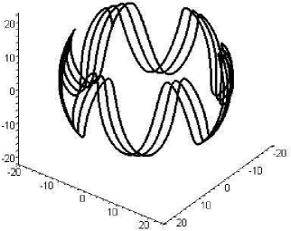
Figure 1: initial conditions: $p^{1}(0)=15$, $p^{2}(0)=-12.13$, $p^{3}(0)=-10$, $J^{1}(0)=1$, $J^{2}(0)=-4$, $J^{3}(0)=3$. Moments of inertia: $B_{1}=1$, $B_{3}=\sec(0.1)^{2}$.

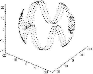
Figure 2: input parameters: $p^{1}(0)=15$, $p^{2}(0)=-12.13$, $p^{3}(0)=-10$, $J^{1}(0)=1$, $J^{2}(0)=-4$, $J^{3}(0)=3$, $\lambda_{0}=0.1$, $\epsilon=0.1$.

4.1 Integrating the Bäcklund: special examples

Let us assume to have a smooth transformation, that we indicate with $\tilde{x}=f(x,\epsilon)$, where the parameter $\epsilon$ plays the role of the time step, such that $f(x,0)=x$. By $\tilde{x}^{n}$ we denote the $n$-th iteration of the map, so that $\tilde{x}^{0}=x$, $\tilde{x}^{1}=f(x,\epsilon)$, $\tilde{x}^{2}=f(f(x,\epsilon),\epsilon)$ and so on. Solving the Bäcklund map amounts to find $\tilde{x}^{n}$ as a function of $x$, $n$ and $\epsilon$. Now we will show that, under given assumptions, there is indeed a positive answer to this question. We will follow a simple argument, well known in group theory [12].

Suppose to do a transformation from $x$ to $\tilde{x}^{1}$ with parameter $\epsilon_{1}$ and then another one from $\tilde{x}^{1}$ to $\tilde{x}^{2}$ with parameter $\epsilon_{2}$. Suppose also that there exist a parameter $\epsilon_{3}$ linking directly $x$ to $\tilde{x}^{2}$. As the Bäcklund are smooth, varying continuously $\epsilon_{1}$ or $\epsilon_{2}$ corresponds to a continuous variation in $\epsilon_{3}$: the Bäcklund transformations define $\epsilon_{3}$ as a continuous function of $\epsilon_{1}$ and $\epsilon_{2}$, say $\epsilon_{3}=\chi(\epsilon_{1},\epsilon_{2})$. Now consider infinitesimal transformations: a small change in the parameter $\epsilon$ take the point $\tilde{x}^{1}$ to a near point $\tilde{x}^{1}+d\tilde{x}^{1}$:

$$\tilde{x}^{1}+d\tilde{x}^{1}=f(x,\epsilon+d\epsilon).$$

But we can arrive at the same point by starting from $\tilde{x}^{1}$ and acting on it with a transformation near the identity, say with the small parameter $\delta\epsilon$:

$$\tilde{x}^{1}+d\tilde{x}^{1}=f(\tilde{x}^{1},\delta\epsilon).$$ (4.5)

The relation between the parameters now reads:

$$\epsilon+d\epsilon=\chi(\epsilon,\delta\epsilon).$$

Obviously $\chi(\epsilon,0)=\epsilon$, so:

$$d\epsilon=\left.\frac{\partial\chi}{\partial\delta\epsilon}\right|_{\delta\epsilon=0}\delta\epsilon\doteq\tau(\epsilon)\delta\epsilon.$$ (4.6)

The relation (4.5) tells us that:

$$d\tilde{x}^{1}=\left.\frac{\partial f(\tilde{x}^{1},\delta\epsilon)}{\partial\delta\epsilon}\right|_{\delta\epsilon=0}\delta\epsilon\doteq\zeta(\tilde{x}^{1})\delta\epsilon.$$

The last expression together with (4.6) gives:

$$\int_{x}^{\tilde{x}^{1}}\frac{dy}{\zeta(y)}=\int_{0}^{\epsilon}\frac{d\lambda}{\tau(\lambda)}\doteq T.$$ (4.7)

This means that there exists a function, say $V$, such that:

$$V(\tilde{x}^{1})=V(x)+T\quad\Longrightarrow\quad V(\tilde{x}^{n})=V(x)+nT.$$

Formally we can write this expression as $\tilde{x}^{n}=V^{-1}(V(x)+nT)$. However, for $n=1$ we must have $\tilde{x}^{1}=f(x,\epsilon(T))$, yielding $\tilde{x}^{n}=f(x,\epsilon(nT))$. The continuous flow discretized is simply given by $x(t)=f(x,\epsilon(t))$ where $x$ is the initial condition ($x(t=0)=x$).

In the following we will present two particular cases, both corresponding to periodic flows, where the Bäcklund transformations can be explicitly integrated.

Example 4.1.

Consider the invariant submanifold $\mathbf{p}=(X,0,Z)$, $\mathbf{J}=(0,Y,0)$. Since now $H_{0}=0$, the freedom to have a parameter $\lambda_{0}$ in (4.2) is just a scaling in time, so we can freely fix it: by now we pose $\lambda_{0}=\frac{\pi}{2}$. With this choice the interpolating Hamiltonian flow discretized by the maps (3.6) is given simply by $\mathcal{H}=\sqrt{Y^{2}+Z^{2}}$. So, as seen at the beginning of this section, in order to have real transformations we pose $\lambda_{1}=\frac{\pi}{2}+i\epsilon$ and $\lambda_{2}=\frac{\pi}{2}-i\epsilon$. The Bäcklund transformation can be now conveniently written in terms of a single function $R$ of $\epsilon$, $X$, $Y$ and $Z$:

$$\tilde{X}=\frac{4R\sinh(\epsilon)(R^{2}+1)}{(R^{2}-1)^{2}+4\cosh(\epsilon)^{2}R^{2}}Z+\frac{(R^{2}+1)^{2}-4R^{2}\sinh(\epsilon)^{2}}{(R^{2}-1)^{2}+4R^{2}\cosh(\epsilon)^{2}}X,$$ (4.8a)

$$\tilde{Y}=\frac{4R\cosh(\epsilon)(R^{2}-1)}{(R^{2}-1)^{2}+4\cosh(\epsilon)^{2}R^{2}}Z-\frac{(R^{2}-1)^{2}-4R^{2}\cosh(\epsilon)^{2}}{(R^{2}-1)^{2}+4R^{2}\cosh(\epsilon)^{2}}Y,$$ (4.8b)

$$\tilde{Z}=\frac{(R^{2}+1)^{2}-4R^{2}\sinh(\epsilon)^{2}}{(R^{2}-1)^{2}+4R^{2}\cosh(\epsilon)^{2}}Z-\frac{4R\sinh(\epsilon)(R^{2}+1)}{(R^{2}-1)^{2}+4\cosh(\epsilon)^{2}R^{2}}X,$$ (4.8c)

$$R\doteq\frac{Z-\sqrt{(\mathcal{H}^{2}\cosh(\epsilon)^{2}-2C_{2}\sinh(\epsilon)^{2})}}{X\sinh(\epsilon)+Y\cosh(\epsilon)}.$$

Note that the two constants under square root in the numerator of $R$ are the Hamiltonian $\mathcal{H}=\sqrt{Y^{2}+Z^{2}}$ and the Casimir function $C_{2}=\frac{X^{2}+Z^{2}}{2}$. To solve the recurrences (4.8) one has to find $\epsilon$ as a function of the parameter $T$ defined in (4.7). To this end we first note that $\left.\frac{d\tilde{Z}}{d\epsilon}\right|_{\epsilon=0}=\frac{2XY}{\mathcal{H}}$, so that by the relations (4.7) we have:

$$\int^{\tilde{Z}}_{Z}\mathcal{H}\frac{d\tilde{Z}}{2\tilde{X}\tilde{Y}}=\int_{0}^{\epsilon}\mathcal{H}\frac{1}{2\tilde{X}\tilde{Y}}\frac{d\tilde{Z}}{d\epsilon}d\epsilon=\int_{0}^{\epsilon}\mathcal{H}\frac{d\epsilon}{\sqrt{\mathcal{H}^{2}\cosh(\epsilon)^{2}-2C_{2}\sinh(\epsilon)^{2}}}=T.$$ (4.9)

All that we have to do now is to perform the integral, invert the result to find $\epsilon$ as a function of $T$, then plug the result into (4.8) and replace $T$ by $nT$: this gives the solution to the Bäcklund recurrences. After some manipulations with the Jacobian elliptic functions we arrive at the simple result:

$$\cosh(\epsilon)=\frac{1}{\textrm{cn}\big{(}T,\frac{\sqrt{2C_{2}}}{\mathcal{H}}\big{)}},\qquad\sinh(\epsilon)=\frac{\textrm{sn}\big{(}T,\frac{\sqrt{2C_{2}}}{\mathcal{H}}\big{)}}{\textrm{cn}\big{(}T,\frac{\sqrt{2C_{2}}}{\mathcal{H}}\big{)}}.$$

With this position we can write down the expressions for $\tilde{X}^{n}$, $\tilde{Y}^{n}$ and $\tilde{Z}^{n}$:

$$\tilde{X}^{n}=\frac{4R\textrm{sn}(nT)\textrm{cn}(nT)(R^{2}+1)}{(R^{2}-1)^{2}\textrm{cn}(nT)^{2}+4R^{2}}Z+\frac{(R^{2}+1)^{2}\textrm{cn}(nT)^{2}-4R^{2}\textrm{sn}(nT)^{2}}{(R^{2}-1)^{2}\textrm{cn}(nT)^{2}+4R^{2}}X,$$

$$\tilde{Y}^{n}=\frac{4R\textrm{cn}(nT)(R^{2}-1)}{(R^{2}-1)^{2}\textrm{cn}(nT)^{2}+4R^{2}}Z-\frac{(R^{2}-1)^{2}\textrm{cn}(nT)^{2}-4R^{2}}{(R^{2}-1)^{2}\textrm{cn}(nT)^{2}+4R^{2}}Y,$$

$$\tilde{Z}^{n}=\frac{(R^{2}+1)^{2}\textrm{cn}(nT)^{2}-4R^{2}\textrm{sn}(nT)^{2}}{(R^{2}-1)^{2}\textrm{cn}(nT)^{2}+4R^{2}}Z-\frac{4R\textrm{sn}(nT)\textrm{cn}(nT)(R^{2}+1)}{(R^{2}-1)^{2}\textrm{cn}(nT)^{2}+4R^{2}}X,$$

$$R=\frac{Z\textrm{cn}(nT)-\sqrt{(\mathcal{H}^{2}-2C_{2}\textrm{sn}(nT)^{2})}}{X\textrm{sn}(nT)+Y},$$

where for brevity we have omitted the elliptic modulus $\frac{\sqrt{2C_{2}}}{\mathcal{H}}$ in the Jacobian elliptic functions “sn” and “cn”. Note that if we pose in (4.9) $2T=t$, that is

$$\cosh(\epsilon)=\frac{1}{\textrm{cn}\big{(}\frac{t}{2},\frac{\sqrt{2C_{2}}}{\mathcal{H}}\big{)}},\qquad\sinh(\epsilon)=\frac{\textrm{sn}\big{(}\frac{t}{2},\frac{\sqrt{2C_{2}}}{\mathcal{H}}\big{)}}{\textrm{cn}\big{(}\frac{t}{2},\frac{\sqrt{2C_{2}}}{\mathcal{H}}\big{)}}$$

in (4.8), then we have the general solution of the dynamical system ruled by the interpolating Hamiltonian flow $\mathcal{H}=\sqrt{Z^{2}+Y^{2}}$, that is the value that takes the hamiltonian $\gamma(\lambda_{0})$ (4.3) on the invariant submanifold considered in this example for $\lambda_{0}$=$\frac{\pi}{2}$. The equations of motion are given by $\mathcal{H}\dot{X}=-YZ$, $\mathcal{H}\dot{Y}=-XZ$, $\mathcal{H}\dot{Z}=XY$.

Obviously this general solution coincide with that found by a direct integration of the previous equation of motion, i.e. with $Z=\sqrt{2C_{2}}\,\textrm{sn}(t+v)$, $X=\sqrt{2C_{2}}\,\textrm{cn}(t+v)$ and $Y=\mathcal{H}\textrm{dn}(t+v)$, where the elliptic modulus of this functions is again $\frac{\sqrt{2C_{2}}}{\mathcal{H}}$ and where $v$ is such that $\textrm{sn}(v)=\frac{Z}{\sqrt{2C_{2}}}$.

Example 4.2.

In the next example we consider the invariant submanifold $\mathbf{p}=(x,y,0)$, $\mathbf{J}=(0,0,z)$. Again, in order to have real transformations we pose $\lambda_{1}=\lambda_{0}+i\epsilon$ and $\lambda_{2}=\lambda_{0}-i\epsilon$ with $\lambda_{0}$ and $\epsilon$ real. In terms of $p^{\pm}=x\pm i\,y$, the maps (3.6) become:

$$\tilde{p}^{-}=\frac{z\sin(\lambda_{0}-i\epsilon)-\sqrt{z^{2}\sin(\lambda_{0}-i\epsilon)^{2}+p^{-}p^{+}}}{z\sin(\lambda_{0}+i\epsilon)-\sqrt{z^{2}\sin(\lambda_{0}+i\epsilon)^{2}+p^{-}p^{+}}}p^{-},$$

$$\tilde{p}^{+}=\frac{z\sin(\lambda_{0}+i\epsilon)-\sqrt{z^{2}\sin(\lambda_{0}+i\epsilon)^{2}+p^{-}p^{+}}}{z\sin(\lambda_{0}-i\epsilon)-\sqrt{z^{2}\sin(\lambda_{0}-i\epsilon)^{2}+p^{-}p^{+}}}p^{+},\qquad\tilde{z}=z.$$ (4.10)

To find the relation defining the parameter $T$ (4.7), first find the expression of $\left.\frac{d\tilde{p}^{-}}{d\epsilon}\right|_{\epsilon=0}$:

$$\left.\frac{d\tilde{p}^{-}}{d\epsilon}\right|_{\epsilon=0}=\frac{2iz\cos(\lambda_{0})p^{-}}{\sqrt{z^{2}\sin(\lambda_{0})^{2}+p^{+}p^{-}}},$$

then by using (4.7) one has:

$$\frac{\sqrt{z^{2}\sin(\lambda_{0})^{2}+p^{+}p^{-}}}{2\cos(\lambda_{0})}\int^{\tilde{p}^{-}}_{p^{-}}\frac{d\tilde{p}^{-}}{iz\tilde{p}^{-}}=T=\frac{\sqrt{z^{2}\sin(\lambda_{0})^{2}+p^{+}p^{-}}}{2\cos(\lambda_{0})}$$

$$\qquad{}\times\int_{0}^{\epsilon}\left(\frac{\cos(\lambda_{0}+i\epsilon)}{\sqrt{z^{2}\sin(\lambda_{0}+i\epsilon)^{2}+p^{+}p^{-}}}+\frac{\cos(\lambda_{0}-i\epsilon)}{\sqrt{z^{2}\sin(\lambda_{0}-i\epsilon)^{2}+p^{+}p^{-}}}\right)d\epsilon$$

or more explicitly:

$$\frac{2i\cos(\lambda_{0})T}{\sqrt{z^{2}\sin(\lambda_{0})^{2}+p^{+}p^{-}}}=\textrm{arcsinh}\left(\frac{z}{\sqrt{p^{+}p^{-}}}\sin(\lambda_{0}+i\epsilon)\right)\!-\textrm{arcsinh}\left(\frac{z}{\sqrt{p^{+}p^{-}}}\sin(\lambda_{0}-i\,\epsilon)\right)$$

$$\hphantom{\frac{2i\cos(\lambda_{0})T}{\sqrt{z^{2}\sin(\lambda_{0})^{2}+p^{+}p^{-}}}}{}=\ln\left(\frac{z\sin(\lambda_{0}-i\epsilon)-\sqrt{z^{2}\sin(\lambda_{0}-i\epsilon)^{2}+p^{-}p^{+}}}{z\sin(\lambda_{0}+i\epsilon)-\sqrt{z^{2}\sin(\lambda_{0}+i\epsilon)^{2}+p^{-}p^{+}}}\right).$$

The Bäcklund transformations (4.10) now take the simple form:

$$\tilde{p}^{-}=\exp\left(\frac{2i\cos(\lambda_{0})zT}{\sqrt{z^{2}\sin(\lambda_{0})^{2}+p^{+}p^{-}}}\right)p^{-},\qquad\tilde{p}^{+}=\exp\left(-\frac{2i\cos(\lambda_{0})zT}{\sqrt{z^{2}\sin(\lambda_{0})^{2}+p^{+}p^{-}}}\right)p^{+},$$

$$\tilde{z}=z,$$

so that again, as expected, the $n$-th iteration of the maps $(\tilde{p}^{-})^{n}$, $(\tilde{p}^{+})^{n}$, $\tilde{z}^{n}$ is found by substituting $T$ with $nT$. By posing $2T=t$ in the previous expressions and returning to the real variables $x=\frac{p^{+}+p^{-}}{2}$ and $y=\frac{p^{+}-p^{-}}{2i}$, we have the continuous flow:

$$x(t)=x\cos\left(\frac{\cos(\lambda_{0})z}{\sqrt{z^{2}\sin(\lambda_{0})^{2}+p^{+}p^{-}}}t\right)+y\sin\left(\frac{\cos(\lambda_{0})z}{\sqrt{z^{2}\sin(\lambda_{0})^{2}+p^{+}p^{-}}}t\right),$$

$$y(t)=y\cos\left(\frac{\cos(\lambda_{0})z}{\sqrt{z^{2}\sin(\lambda_{0})^{2}+p^{+}p^{-}}}t\right)-x\sin\left(\frac{\cos(\lambda_{0})z}{\sqrt{z^{2}\sin(\lambda_{0})^{2}+p^{+}p^{-}}}t\right)$$

corresponding to the general solution of the continuous system ruled by the value that takes the hamiltonian $\gamma(\lambda_{0})$ (4.3) on the invariant submanifold $\mathbf{p}=(x,y,0)$, $\mathbf{J}=(0,0,z)$ considered in this example.

Appendix A Integration of the continuous model

For the sake of completeness, we report here the solution to the evolution equations defining the Kirchhoff top. Gustav Kirchhoff in his “Vorlesungen über mathematische Physik” [2] deals with the problem of integrating equations of motion (1.4). For the physical variables $(J^{1},J^{2},J^{3})$ and $(p^{1},p^{2},p^{3})$ they are written in extended form as:

$$\dot{p}^{1}(t)=\alpha J^{3}(t)p^{2}(t)-\beta J^{2}(t)p^{3}(t),\qquad\dot{p}^{2}(t)=\beta J^{1}(t)p^{3}(t)-\alpha p^{1}(t)J^{3}(t),$$

$$\dot{p}^{3}(t)=\beta\big{(}J^{2}(t)p^{1}(t)-J^{1}(t)p^{2}(t)\big{)},$$

$$\dot{J}^{1}(t)=(\alpha-\beta)J^{2}(t)J^{3}(t)+\beta p^{2}(t)p^{3}(t),\qquad\dot{J}^{2}(t)=(\beta-\alpha)J^{1}(t)J^{3}(t)-\beta p^{1}(t)p^{3}(t),$$

$$\dot{J}^{3}(t)=0\quad\Rightarrow\quad J^{3}={\rm const}\doteq M,$$

where for simplicity we have posed $\alpha\doteq B_{3}^{-1}$ and $\beta\doteq B_{1}^{-1}$. The new variables suggested by Kirchhoff are given by $p^{1}=s\cos(f)$, $p^{2}=s\sin(f)$, $J^{1}=\sigma\cos(\psi+f)$, $J^{2}=\sigma\sin(\psi+f)$. In terms of these variables the equations of motion can be written as:

$$\dot{s}(\tau)=-\sigma(\tau)p^{3}(\tau)\sin(\psi(\tau)),\qquad\dot{\sigma}(\tau)=-s(\tau)p^{3}(\tau)\sin(\psi(\tau)),$$

$$\dot{p}^{3}(\tau)=s(\tau)\sigma(\tau)\sin(\psi(\tau)),$$

$$\dot{\psi}(\tau)=M-p^{3}(\tau)\cos(\psi(\tau))\left(\frac{\sigma(\tau)}{s(\tau)}+\frac{s(\tau)}{\sigma(\tau)}\right),\qquad\dot{f}(\tau)=\frac{\sigma(\tau)}{s(\tau)}p^{3}(\tau)\cos(\psi(\tau))-\frac{\alpha}{\beta}M,$$

where $\tau\doteq\beta t$, $(\,^{\dot{}}\,)=\frac{\partial(\,\,)}{\partial\tau}$. By using the constraints given by the Casimirs and the integral $H_{1}$, i.e. $2H_{1}=\sigma^{2}+(p^{3})^{2}$, $2C_{2}=s^{2}+(p^{3})^{2}$, $s\sigma\cos(\psi)+Mp^{3}=C_{1}$, one can readily obtains the equation for the evolution of $p^{3}$:

$$\big{(}\dot{p}^{3}\big{)}^{2}=\big{(}\big{(}p^{3}\big{)}^{2}-2C_{2}\big{)}\big{(}\big{(}p^{3}\big{)}^{2}-2H_{1}\big{)}-\big{(}Mp^{3}-C_{1}\big{)}^{2}.$$ (A.1)

At this point Kirchhoff notes that this equation is integrable and that one can obtain by the expression of $p^{3}$ those for the other variables, but soon after he passes to consider the special case $J^{1}=J^{3}=p^{2}=0$. At our knowledge the first author to integrate this system was G.E. Halphen in 1886 [13], also if some authors gives Kirchhoff as reference for the complete integration of the equation of motions. The expression for $p^{3}(t)$ of Halphen is written in terms of Weierstrass $\wp$ function; it reads as:

$$p^{3}(\tau)=\frac{1}{2}\left(\frac{\dot{\wp}\big{(}\tau+K,\Phi+3\Psi^{2},\Psi^{3}-\Psi\Phi-\Omega^{3}\big{)}-\Omega}{\wp\big{(}\tau+K,\Phi+3\Psi^{2},\Psi^{3}-\Psi\Phi-\Omega^{3}\big{)}-\Psi}\right),$$ (A.2)

where

$$\Psi=\frac{2C_{2}+2C_{1}+M^{2}}{6},\qquad\Omega=\frac{MC_{1}}{2},\qquad\Phi=4C_{2}H_{1}-C_{1}^{2}.$$

Note that the last two arguments of $\wp$ are not its periods but the elliptic invariants. In order to fit with the given initial condition $p^{3}(0)$ it is possible to show that one has to choose the value of $K$ according to the relation:

$$\wp\big{(}K,\Phi+3\Psi^{2},\Psi^{3}-\Psi\Phi-\Omega^{3}\big{)}=\frac{\big{(}p^{3}(0)\big{)}^{2}+\dot{p}^{3}|_{t=0}-\Psi}{2}.$$

By the expression (A.2) it isn’t simple to see that $p^{3}(\tau)$ is actually bounded. It is however possible to make plain this point by writing the solution in terms of the roots of (A.1). Let us clarify this statement. The key observation is that if one looks at the r.h.s. of (A.1) as an algebraic equation for $p^{3}$, so that the equation is a quartic in this variable, then it is possible to show that it has always four real roots. This allows to arrange them in order of crescent magnitude and then to infer from this fact some properties of the solution of (A.1). The Casimirs and integrals are fixed if one fixes the initial conditions, so we can assume that the dynamical variables in these quantities are specified by their initial values, say at $\tau=0$. With this in mind, by posing $p^{3}(\tau)=x$ we rewrite (A.1) as:

$$\big{(}x^{2}-2C_{2}\big{)}\big{(}x^{2}-2H_{1}\big{)}-\big{(}Mx-C_{1}\big{)}^{2}=f(x).$$ (A.3)

If we can find five distinct points where $f(x)$ changes its sign, then the l.h.s. of equation (A.3) has four real roots. These points are collected in Table 1.

Table 1: The changes in the sign of $f(x)$.

$x$	$f(x)$
$+\infty$	$>0$
$\sqrt{C_{2}+H_{1}}$	$\leq 0$
$p^{3}(0)$	$\geq 0$
$-\sqrt{C_{2}+H_{1}}$	$\leq 0$
$-\infty$	$>0$

Note that iff the initial condition are such that $J^{1}(0)=J^{2}(0)=p^{1}(0)=p^{2}(0)=0$, then $p^{3}(0)$ is equal to one of the two points $\pm\sqrt{C_{2}+H_{1}}$. But in this case the four roots are $x=p^{3}(0)$, $x=J^{3}(0)-p^{3}(0)$, $x=-J^{3}(0)-p^{3}(0)$, with $x=p^{3}(0)$ a double root, so that also in this case there are four real roots. So in general the l.h.s. of (A.3) has four real roots, with at most three equals and with at least one negative (for obvious reasons we do not consider the trivial case when all the dynamical variables are initially equal to zero). Given the reality of the roots, it is possible now to sort them in an increasing order of magnitude so that by labelling with $a$, $b$, $c$, $d$, we can assume $a\geq b\geq c\geq d$. Note also that $p^{3}(0)$ lies in the interval $(c,b)$. Equation (A.1) can be written then as:

$$(\dot{p}^{3})^{2}=(p^{3}-a)(p^{3}-b)(p^{3}-c)(p^{3}-d).$$ (A.4)

The integration of (A.4) is reduced to a standard elliptic integral of the first kind by the substitution [14] $z^{2}=\frac{(b-p^{3}(\tau))(a-c)}{(a-p^{3}(\tau))(b-c)}$. After some algebra we obtain:

$$p^{3}(\tau)=\frac{b-\mu^{2}a\,\textrm{sn}(v+\eta\tau,k)^{2}}{1-\mu^{2}\,\textrm{sn}(v+\eta\tau,k)^{2}},$$ (A.5)

where

$$\mu^{2}=\frac{b-c}{a-c},\qquad k^{2}=\frac{(a-d)(b-c)}{(a-c)(b-d)},\qquad\eta^{2}=\frac{(a-c)(b-d)}{4},$$

$$v=\textrm{sn}^{-1}\left(\sqrt{\frac{(b-p^{3}(0))(a-c)}{(a-p^{3}(0))(b-c)}},k\right).$$

The symbol “sn” denotes the Jacobi elliptic function of modulus $k$. As can be seen by the expansion of $p^{3}(\tau)$ in the neighborhood of $\tau=0$, the sign of $\eta$ has to be chosen according to the sign of $\dot{p}^{3}(0)$, i.e. $\textrm{sgn}(\eta)=-\textrm{sgn}(\dot{p}^{3}(0))=-\textrm{sgn}\big{(}J^{2}(0)p^{1}(0)-J^{1}(0)p^{2}(0)\big{)}$. Note that $p^{3}(\tau)$ is bounded in the set $(c,a)$, that is $c\leq p^{3}(\tau)\leq a$. Having (A.5) it is a simple matter to write down the expressions for the other dynamical variables:

$$s(\tau)=\sqrt{2C_{2}-(p^{3}(\tau))^{2}},\qquad\sigma(\tau)=\sqrt{2H_{1}-(p^{3}(\tau))^{2}},\qquad\cos(\psi(\tau))=\frac{C_{1}-Mp^{3}(\tau)}{s(\tau)\sigma(\tau)},$$

$$f(\tau)=f(0)+\int_{0}^{\tau}\left(\frac{s(z)}{\sigma(z)}p^{3}(z)\cos(\psi(z))-\frac{\alpha}{\beta}M\right)dz.$$

The continuous flow is in general quasi-periodic. One can ask what are the conditions under which the flow becomes periodic. Note that $p^{3}(\tau)$, $s(\tau)$, $\sigma(\tau)$ and $\cos(\psi(\tau))$ are all periodic functions with the same period (obviously we are interested only in real periods). Such period is given by

$$\mathcal{T}=\frac{2K(k)}{\eta},$$ (A.6)

and depends only on the initial conditions and not on the parameters $\alpha$ and $\beta$ of the model. In (A.6) $K(k)$ is the complete elliptic integral of first kind [14], $k$ and $\eta$ are as given in (A.5). If the function $f(\tau)$ is such that

$$f(\tau+n\mathcal{T})=f(\tau)+2m\pi,\qquad(n,m)\in\mathbb{Z}^{2}$$ (A.7)

then it isn’t difficult to see that the motion is indeed completely periodic. In this case the trajectories of the moving point ($p^{1}(\tau),p^{2}(\tau),p^{3}(\tau)$), constrained on the two-sphere with constant radius given by $r^{2}=\mathbf{p}(\tau)\cdot\mathbf{p}(\tau)$, close. The condition (A.7) is equivalent to the following constraint on the ratio of the parameters $\alpha$ and $\beta$:

$$\frac{\alpha}{\beta}=\frac{\int_{0}^{\mathcal{T}}\Big{(}\frac{s(z)}{\sigma(z)}p^{3}(z)\cos(\psi(z))\Big{)}dz-\frac{2m\pi}{n}}{M\,\mathcal{T}}.$$

Acknowledgments

We are grateful to both referees for their constructive comments and criticisms, and in particular to one of them for his crucial remarks and for having brought to our attention the article [11].

The research underlying this paper has been partially supported by the Italian MIUR, Research Project “Integrable Nonlinear Evolutions, continuous and discrete: from Water Waves downwards to Symplectic Map”, Prot. n. 20082K9KXZ/005, in the framework of the PRIN 2008: “Geometrical Methods in the Theory of Nonlinear Waves and Applications”.

References

- [1]
- [2] Kirchhoff G., Vorlesungen über mathematische Physik, Neunzenthe Vorlesung, Teubner, Leipzig, 1876, 233–250.
- [3] Milne-Thomson L.M., Theoretical hydrodynamics, Dover Publications, 1996.
- [4] Lamb H., Hydrodynamics, Cambridge University Press, Cambridge, 1993.
-
[5]
Gaudin M., Diagonalisation d’une classe d’hamiltoniens de spin,
J. Physique 37 (1976), 1087–1098.
Gaudin M., La function d’onde de Bethe, Masson, Parigi, 1983. - [6] Musso F., Petrera M., Ragnisco O., Algebraic extension of Gaudin models, J. Nonlinear Math. Phys. 12 (2005), suppl. 1, 482–498, nlin.SI/0410016.
- [7] Petrera M., Ragnisco O., From Gaudin models to integrable tops, SIGMA 3 (2007), 058, 14 pages, math-ph/0703044.
- [8] Faddeev L.D., Takhtajan L.A., Hamiltonian methods in the theory of solitons, Springer Series in Soviet Mathematics, Springer-Verlag, Berlin, 1987.
- [9] Kuznetsov V.B., Sklyanin E.K., On Bäcklund transformations for many-body systems, J. Phys. A: Math. Gen. 31 (1998), 2241–2251, solv-int/9711010.
- [10] Ragnisco O., Zullo F., Bäcklund transformation as exact integrable time-discretizations for the trigonometric Gaudin model, J. Phys. A: Math. Theor. 43 (2010), 434029, 14 pages, arXiv:1003.0389.
- [11] Kuznetsov V.B., Vanhaecke P., Bäcklund transformations for finite-dimensional integrable systems: a geometric approach, J. Geom. Phys. 44 (2002), 1–40, nlin.SI/0004003.
- [12] Hamermesh M., Group theory and its application to physical problems, Dover Publications, 1989.
- [13] Halphen G.E., Traité des fonctions elliptiques et de leurs applications, Vol. 2, Paris, Gauthier-Villars, 1886.
- [14] Armitage J.V., Eberlein W.F., Elliptic functions, London Mathematical Society Student Texts, Vol. 67, Cambridge University Press, Cambridge, 2006.