An Unstaggered Constrained Transport Method for the 3D Ideal Magnetohydrodynamic Equations

Abstract

Numerical methods for solving the ideal magnetohydrodynamic (MHD) equations in more than one space dimension must either confront the challenge of controlling errors in the discrete divergence of the magnetic field, or else be faced with nonlinear numerical instabilities. One approach for controlling the discrete divergence is through a so-called constrained transport method, which is based on first predicting a magnetic field through a standard finite volume solver, and then correcting this field through the appropriate use of a magnetic vector potential. In this work we develop a constrained transport method for the 3D ideal MHD equations that is based on a high-resolution wave propagation scheme. Our proposed scheme is the 3D extension of the 2D scheme developed by Rossmanith [SIAM J. Sci. Comp. 28, 1766 (2006)], and is based on the high-resolution wave propagation method of Langseth and LeVeque [J. Comp. Phys. 165, 126 (2000)]. In particular, in our extension we take great care to maintain the three most important properties of the 2D scheme: (1) all quantities, including all components of the magnetic field and magnetic potential, are treated as cell-centered; (2) we develop a high-resolution wave propagation scheme for evolving the magnetic potential; and (3) we develop a wave limiting approach that is applied during the vector potential evolution, which controls unphysical oscillations in the magnetic field. One of the key numerical difficulties that is novel to 3D is that the transport equation that must be solved for the magnetic vector potential is only weakly hyperbolic. In presenting our numerical algorithm we describe how to numerically handle this problem of weak hyperbolicity, as well as how to choose an appropriate gauge condition. The resulting scheme is applied to several numerical test cases.

1 Introduction

The ideal magnetohydrodynamic (MHD) equations are a common model for the macroscopic behavior of collisionless plasma [8, 19, 28]. These equations model the fluid dynamics of an interacting mixture of positively and negatively charged particles, where each species is assumed to behave as a charged ideal gas. Under the MHD assumption, this mixture is taken to be quasi-neutral, meaning that as one species moves, the other reacts instantaneously. This assumption allows one to collapse what should be two sets of evolution equation into a single set of equations for the total mass, momentum, and energy of the mixture. Furthermore, the resulting dynamics are assumed to happen on slow time scales compared to the propagation time of light waves, which yields a simplified set of Maxwell equations. Finally, the term ideal refers to the fact that we assume the ideal Ohm’s law: ${\bf E}={\bf B}\times{\bf u}$, which removes any explicit resistivity and the Hall term.

All of the above described simplifications conspire to turn the original two-fluid plasma model into a system that can be viewed as a modified version of the compressible Euler equations from gas dynamics. In particular, the ideal MHD system can be written as a system of hyperbolic conservation laws, where the conserved quantities are mass, momentum, energy, and magnetic field. Furthermore, this system is equipped, just as the compressible Euler equations are, with an entropy inequality that features a convex scalar entropy and a corresponding entropy flux. Indeed, the scalar entropy, with some help from the fact that the magnetic field is divergence-free, can be used to define entropy variables in which the MHD system is in symmetric hyperbolic form [5, 18].

As has been noted many times in the literature (e.g., Brackbill and Barnes [6], Evans and Hawley [14], and Tóth [40]), numerical methods for ideal MHD must in general satisfy (or at least control) some discrete version of the divergence-free condition on the magnetic field:

$$\nabla\cdot{\bf B}=0.$$ (1)

Failure to accomplish this generically leads to a nonlinear numerical instability, which often leads to negative pressures and/or densities. Starting with the paper of Brackbill and Barnes [6] in 1980, several approaches for controlling errors in $\nabla\cdot{\bf B}$ have been proposed. An in-depth review of many of these methods can be found in Tóth [40]. We very briefly summarize the main points below.

Projection methods.

Projection methods for ideal MHD are based on a predictor-corrector approach for the magnetic field. Some standard finite volume or finite difference method is used to solve the ideal MHD equations from time $t^{n}$ to $t^{n+1}$. The approximate magnetic field that is predicted at time $t^{n+1}$ is denoted by ${\bf B}^{\star}$. In general, ${\bf B}^{\star}$ contains both a nontrivial divergence-free subspace and a divergent subspace; one would like to extract only the divergence-free part and discard the divergent part. This can be accomplished by setting

$${\bf B}^{n+1}:={\bf B}^{\star}-\nabla\psi,$$ (2)

and forcing $\nabla\cdot{\bf B}^{n+1}=0$, which results in a Poisson equation for the scalar potential $\psi$:

$$\nabla^{2}\psi=\nabla\cdot{\bf B}^{\star}.$$ (3)

Once $\psi$ is computed, the divergence-free magnetic field at time $t^{n+1}$ is taken to be (2) (see Tóth [40] and Balsara and Kim [3] for further discussion).

This method is attractive for it allows a variety of methods to be used in the prediction step, and then only requires one Poisson solve per time-step to correct it. The clear disadvantage of this approach is that it requires a global elliptic solve on a problem, ideal MHD, that is purely hyperbolic. This could be especially computationally inefficient in the case of adaptively refined grids.

The 8-wave formulation.

The linearized ideal MHD equations support seven propagating plane-wave solutions and a stationary plane-wave solution. The stationary plane-wave solution comes directly from the fact that the (nonlinear) MHD equations preserve the divergence constraint:

$$\left(\nabla\cdot{\bf B}\right)_{,t}=0,$$ (4)

where $,t$ denotes the partial derivative with respect to time. A seemingly unrelated fact was proved by Godunov [18]: the ideal MHD can only be put in symmetric hyperbolic form if one adds to the ideal MHD equations a term that is proportional to $\nabla\cdot{\bf B}$ (in effect adding a term that, at least on the continuous level, is zero). As it turns out, this additional “source term” not only allows the equations to be put in symmetric hyperbolic form, but it also restores Galilean invariance. With the additional term the divergence wave is no longer stationary, and instead, it propagates with the fluid velocity:

$$\left(\nabla\cdot{\bf B}\right)_{,t}+\nabla\cdot\left({\bf u}\nabla\cdot{\bf B}\right)=0.$$ (5)

From the point of view of numerical methods, the difference between a stationary and a propagating divergence wave turns out to be very significant. Powell [31] and Powell et al. [32] showed that numerical methods applied to the MHD equations with the symmetrizing “source term” were much more stable than the same methods applied to the original MHD equations. The modified form of the MHD equations has come be called the 8-wave formulation, since this form of the equations supports eight propagating plane wave solutions. Although this approach has been used with some success (see Powell et al. [32]), it does have a significant drawback: the 8-wave formulation is non-conservative and difficulties with obtaining the correct weak solution have been documented in the literature (see for example Tóth [40]).

Hyperbolic divergence cleaning methods.

This method was introduced by Dedner et al. [12], and is a close cousin to the above described projection method. The basic idea is to again solve for the divergence error in the magnetic field. Instead of solving an elliptic equation, however, a damped hyperbolic equation is prescribed for the divergence error. This does not produce an exact divergence-free magnetic field; however, it allows for the divergence error to be propagated and damped away from where it originated. The main advantage of this method is that it is easy to implement and requires no elliptic solve. The main disadvantage is that this approach has two tunable parameters: the speed of propagation of the error and the rate at which the divergence error is damped.

Constrained transport methods.

The constrained transport (CT) approach for ideal MHD was introduced by Evans and Hawley [14]. The method is a modification of Yee’s method [47] for electromagnetic wave propagation, and, at least in its original formulation, introduced staggered magnetic and electric fields. Since the introduction of the CT framework, several variants and modifications have been introduced, including the work of Balsara [2], Balsara and Spicer [4], Dai and Woodward [11], Fey and Torrilhon [15], Londrillo and Del Zanna [26], Rossmanith [35], Ryu et al. [36], and De Sterck [37]. An overview of many of these approaches, as well as the introduction of a few more variants, can be found in Tóth [40]. In particular, Tóth [40] showed that a staggered magnetic field is not necessary.

The CT framework, at least several versions of it, can also be viewed as a kind of predictor-corrector approach for the magnetic field. Roughly speaking, the idea is to again compute all of the conserved quantities with a standard finite volume method. From these computed quantities one then constructs an approximation to the electric field through the ideal Ohm’s law. This electric field can then be used to update the magnetic vector potential, which in turn, can be used to compute a divergence-free magnetic field (see §3 for more details).

The main advantages of this approach are that (1) there is no elliptic solve and (2) there are no free parameters to choose such as in the hyperbolic divergence-cleaning technique.

We focus in this work on developing a constrained transport method for the 3D ideal MHD equations based on the high-resolution wave propagation scheme of LeVeque [23] and its 3D extension developed by Langseth and LeVeque [21]. Our proposed scheme is the 3D extension of the 2D constrained transport scheme developed by Rossmanith [35].

The wave propagation scheme is an unsplit finite volume method that achieves second-order accuracy and optimal stability in higher-dimensions through the use of so-called transverse Riemann solvers. These transverse Riemann solvers are based partly on the work of Colella [9] on corner transport upwind (CTU) methods. It is worth noting that there has been recent work on CTU methods in the context of MHD by Gardiner and Stone [16, 17] and Mignone and Tzeferacos [27]. Gardiner and Stone [16, 17] developed a constrained transport approach, while Mignone and Tzeferacos [27] considered the hyperbolic divergence cleaning method of [12] in the context of the CTU scheme. The method we propose in this work is therefore in the same class of methods as that of Gardiner and Stone [16, 17] (i.e., unsplit finite volume methods with constrained transport), and to a lesser extent Mignone and Tzeferacos [27] (i.e., unsplit methods for MHD), although the details of our base scheme and especially the details of how the magnetic field is updated differ greatly from these approaches.

In particular, the approach for updating the magnetic field that we propose in this work is based on a generalization of the 2D constrained transport scheme of [35], which is equipped with all of the following features:

1. All quantities, including all components of the magnetic field and magnetic potential, are treated as cell-centered;

2. The magnetic potential is evolved alongside the eight conserved MHD variables via a modified non-conservative high-resolution wave propagation scheme; and

3. Special limiters are applied in the evolution of the magnetic potential, which control unphysical oscillations in the magnetic field.

The scheme developed in this work extends all three of the above features to the 3D case. The new challenge that arises in 3D is that the magnetic potential is a vector potential (instead of a scalar as in the 2D case). Furthermore, this vector potential obeys, at least under gauge condition we advocate in this work, a non-conservative weakly hyperbolic evolution equation. We are thus faced with two important challenges:

1. Developing a wave propagation scheme for this non-conservative weakly hyperbolic evolution equation; and

2. Constructing appropriate limiters that again have the effect of limiting the magnetic potential in such a way as to produce a non-oscillatory magnetic field.

After briefly reviewing the MHD equations in §2, we describe an overview of our proposed method in §3. One important issue that arises from this approach is the gauge choice; we discuss several possible choices in §4. Under the gauge condition that we choose, the 3D transport equation that must be solved for the magnetic potential is only weakly hyperbolic. We describe in detail in §5 how to numerically handle this difficulty. The resulting scheme is applied to several numerical test cases in §6.

2 Basic equations

The ideal magnetohydrodynamic (MHD) equations are a classical model from plasma physics that describe the macroscopic evolution of a quasi-neutral two-fluid plasma system. Under the quasi-neutral assumption, the two-fluid equations can be collapsed into a single set of fluid equations for the total mass, momentum, and energy of the system. The resulting equations can be written in the following form:

$$\frac{\partial}{\partial t}\begin{bmatrix}\rho\\ \rho{\bf u}\\ {\mathcal{E}}\\ {\bf B}\end{bmatrix}+\nabla\cdot\begin{bmatrix}\rho{\bf u}\\ \rho{\bf u}{\bf u}+\left({p}+\frac{1}{2}\|{\bf B}\|^{2}\right){\mathbb{I}}-{\bf B}{\bf B}\\ {\bf u}\left({\mathcal{E}}+{p}+\frac{1}{2}\|{\bf B}\|^{2}\right)-{\bf B}\left({\bf u}\cdot{\bf B}\right)\\ {\bf u}{\bf B}-{\bf B}{\bf u}\end{bmatrix}=0,$$ (6)

$$\nabla\cdot{\bf B}=0,$$ (7)

where $\rho$, $\rho{\bf u}$, and ${\mathcal{E}}$ are the total mass, momentum, and energy densities of the plasma system, and ${\bf B}$ is the magnetic field. The thermal pressure, $p$, is related to the conserved quantities through the ideal gas law:

$$p=\left(\gamma-1\right)\left({\mathcal{E}}-\frac{1}{2}\|{\bf B}\|^{2}-\frac{1}{2}\rho\|{\bf u}\|^{2}\right),$$ (8)

where $\gamma=5/3$ is the ideal gas constant.

The equation for the magnetic field comes from Faraday’s law:

$${\bf B}_{,t}+\nabla\times{\bf E}=0,$$ (9)

where the electric field, ${\bf E}$, is approximated by Ohm’s law for a perfect conductor:

$${\bf E}={\bf B}\times{\bf u}.$$ (10)

Note that we have used in the above expression a comma followed by a subscript as short-hand notation for partial differentiation. This notation is standard in many areas of mathematics, most notably in relativity theory (e.g., [30]). We will continue to use this notation throughout this paper.

Under the Ohm’s law assumption, we can rewrite Faraday’s law in the following divergence form:

$${\bf B}_{,t}+\nabla\times\left({\bf B}\times{\bf u}\right)={\bf B}_{,t}+\nabla\cdot\left({\bf u}{\bf B}-{\bf B}{\bf u}\right)=0.$$ (11)

Since the electric field is determined entirely from Ohm’s law, we do not require an evolution equation for it; and thus, the only other piece that we need from Maxwell’s equations is the divergence-free condition on the magnetic field (7). A complete derivation and discussion of MHD system (6)-(7) can be found in several standard plasma physics textbooks (e.g., [8, 19, 28]).

2.1 $\nabla\cdot{\bf B}=0$ is an involution

We first note that system (6), along with the equation of state (8), provides a full set of equations for the time evolution of all eight state variables: $\left(\rho,\,\rho{\bf u},\,{\mathcal{E}},\,{\bf B}\right)$. These evolution equations form a hyperbolic system. In particular, the eigenvalues of the flux Jacobian in some arbitrary direction ${\bf n}$ ($\|{\bf n}\|=1$) can be written as follows:

$$\lambda^{1,8} ={\bf u}\cdot{\bf n}\mp c_{f}$$ : fast magnetosonic waves, (12)

$$\lambda^{2,7} ={\bf u}\cdot{\bf n}\mp c_{a} \acute{\text{e}}$$ : Alfvn waves, (13)

$$\lambda^{3,6} ={\bf u}\cdot{\bf n}\mp c_{s}$$ : slow magnetosonic waves, (14)

$$\lambda^{4} ={\bf u}\cdot{\bf n}$$ : entropy wave, (15)

$$\lambda^{5} ={\bf u}\cdot{\bf n}$$ : divergence wave, (16)

where

$$a \equiv\sqrt{\frac{\gamma p}{\rho}},$$ (17)

$$c_{a} \equiv\sqrt{\frac{\left({\bf B}\cdot{\bf n}\right)^{2}}{\rho}},$$ (18)

$$c_{f} \equiv\left\{\frac{1}{2}\left[a^{2}+\frac{\|{\bf B}\|^{2}}{\rho}+\sqrt{\left(a^{2}+\frac{\|{\bf B}\|^{2}}{\rho}\right)^{2}-4a^{2}\frac{\left({\bf B}\cdot{\bf n}\right)^{2}}{\rho}}\right]\right\}^{1/2},$$ (19)

$$c_{s} \equiv\left\{\frac{1}{2}\left[a^{2}+\frac{\|{\bf B}\|^{2}}{\rho}-\sqrt{\left(a^{2}+\frac{\|{\bf B}\|^{2}}{\rho}\right)^{2}-4a^{2}\frac{\left({\bf B}\cdot{\bf n}\right)^{2}}{\rho}}\right]\right\}^{1/2}\,.$$ (20)

The eigenvalues are well-ordered in the sense that

$$\lambda^{1}\leq\lambda^{2}\leq\lambda^{3}\leq\lambda^{4}\leq\lambda^{5}\leq\lambda^{6}\leq\lambda^{7}\leq\lambda^{8}\,.$$ (21)

The fast and slow magnetosonic waves are genuinely nonlinear, while the remaining waves are linearly degenerate. Note that the so-called divergence-wave has been made to travel at the speed ${\bf u}\cdot{\bf n}$ via the 8-wave formulation described in §1, thus restoring Galilean invariance [18, 31, 32]. Note that despite the fact that we use the eigenvalues and eigenvectors of the 8-wave formulation of the MHD equations, we will still solve the MHD equations in conservative form (i.e., without the Godunov-Powell “source term”).

The additional equation (7) is not needed in the time evolution of the conserved variables in the following sense:

If (7) is true at some time $t=T$, then evolution equation (6) guarantees that (7) is true for all time.

This result follows from taking the divergence of Faraday’s law, which yields:

$$\left(\nabla\cdot{\bf B}\right)_{,t}=0.$$ (22)

For this reason, (7) should not be regarded as constraint (such as the $\nabla\cdot{\bf u}=0$ constraint for the incompressible Navier-Stokes equations), but rather an involution [10].

2.2 The role of $\nabla\cdot{\bf B}=0$ in numerical discretizations

Although $\nabla\cdot{\bf B}=0$ is an involution, and therefore has no dynamic impact on the evolution of the exact MHD system, the story is more complicated for numerical discretizations of ideal MHD. Brackbill and Barnes [6] gave a physical explanation as to why $\nabla\cdot{\bf B}=0$ should be satisfied in some appropriate discrete sense:

If $\nabla\cdot{\bf B}\neq 0$, then the magnetic force,

$${\bf F}=\nabla\cdot\left\{{\bf B}{\bf B}-\frac{1}{2}\|{\bf B}\|^{2}\,{\mathbb{I}}\right\},$$ (23)

in the direction of the magnetic field, will not in general vanish:

$${\bf F}\cdot{\bf B}=\|{\bf B}\|^{2}\,\left(\nabla\cdot{\bf B}\right)\neq 0.$$ (24)

If this spurious forcing becomes too large, it can lead to numerical instabilities (see for example [6, 35, 40]).

Tóth [41] analyzed the magnetic force for central finite difference methods and develop an approach with the property that ${\bf F}\cdot{\bf B}=0$ on the discrete level. This analysis makes it clear that simply having $\nabla\cdot{\bf B}=0$ on the discrete level is not sufficient to guarantee that ${\bf F}\cdot{\bf B}=0$ is satisfied. Londrillo and Del Zanna [26] came to the same conclusion and proposed a modified approach for computing numerical fluxes. However, in [35] it is argued that by satisfying an appropriate discrete form of $\nabla\cdot{\bf B}=0$ the error in ${\bf F}\cdot{\bf B}$ is sufficiently controlled; and therefore, the additional modifications that are proposed in [26] and [41] are not found to be necessary. We omit the details here; and instead, refer the reader to [26, 35, 41].

Another explanation as to why $\nabla\cdot{\bf B}=0$ should not be ignored in numerical discretizations of MHD from a slightly different point-of-view, was offered by Barth [5]. Barth’s explanation is based on the well-known result of Godunov [18] that the MHD entropy density,

$$U(q)=-\rho\log\left(p\rho^{-\gamma}\right),$$ (25)

produces a set of entropy variables, $U_{,q}$, that do not immediately symmetrize the ideal MHD equations. Instead, a symmetric hyperbolic form of ideal MHD can only be obtained if an additional term that is proportional to the divergence of the magnetic field is included in the MHD equations:

$$\underset{\text{ideal MHD}}{\underbrace{q_{,t}+{\nabla}\cdot{\bf F}(q)}}+\underset{\text{additional term}}{\underbrace{\chi_{,q}\,{\nabla}\cdot{\bf B}}}=0,\qquad\text{where}\quad\chi(q)=\left(\gamma-1\right)\frac{\rho{\bf u}\cdot{\bf B}}{p}.$$ (26)

By looking at how the entropy behaves on the discrete level, Barth [5] was able to prove that certain discontinuous Galerkin discretizations of the ideal MHD equtions could be made to be entropy stable (see Tadmor [42]) if the discrete magnetic field where made globally divergence-free. The implication of this result is that schemes that do not control errors in the divergence of the magnetic field run the risk of becoming entropy unstable.

3 An unstaggered constrained transport framework

The constrained transport framework advocated in this work is based on using the magnetic vector potential, ${\bf A}:{{\rm l}\kern-1.49994pt{\rm R}}^{+}\times{{\rm l}\kern-1.49994pt{\rm R}}^{3}\rightarrow{{\rm l}\kern-1.49994pt{\rm R}}^{3}$, whose curl yields the magnetic field:

$${\bf B}=\nabla\times{\bf A}.$$ (27)

A key feature of the proposed method is that the magnetic vector potential is updated alongside the conserved variables: $q=(\rho,\rho{\bf u},{\mathcal{E}},{\bf B})^{T}$.

The use of the magnetic potential in computing solutions to the MHD equations goes all the way back to Wilson [46] in 1975, who considered relativistic 2D axisymmetric problems, and Dorfi [13] in 1986, who considered fully three-dimensional flow. These approaches did not use modern shock-capturing techniques; and therefore, the computed solutions exhibited strong numerical diffusion. The first direct use of the magnetic potential in the context of modern shock-capturing schemes was due to Londrillo and Del Zanna [25]. Subsequent work on using a magnetic potential with shock-capturing schemes includes De Sterck [37], Londrillo and Del Zanna [26], and Rossmanith [35].

The main focus of this work is to extend the 2D constrained transport method introduced by Rossmanith [35] to three-dimensions. We begin with an outline of our method that lists all of the key steps necessary to completely advance the solution from its current state at time $t=t^{n}$ to its new state at time $t=t^{n+1}=t^{n}+\Delta t$:

  Step 0.

Start with the current state:  $\left(\rho^{n},\,\rho{\bf u}^{n},\,{\mathcal{E}}^{n},\,{\bf B}^{n},\,{\bf A}^{n}\right)$.

  Step 1.

Update MHD variables via a standard finite volume scheme:

$$\left(\rho^{n},\,\rho{\bf u}^{n},\,{\mathcal{E}}^{n},\,{\bf B}^{n}\right)\quad\Longrightarrow\quad\left(\rho^{n+1},\,\rho{\bf u}^{n+1},\,{\mathcal{E}}^{\star},\,{\bf B}^{\star}\right),$$

where the energy and magnetic field values, ${\mathcal{E}}^{\star}$ and ${\bf B}^{\star}$, are given a $\star$ superscript instead of $n+1$ to emphasize that these values will be modified by the constrained transport algorithm before the end of the time step.

  Step 2.

Define the time-averaged velocity:  ${\bf u}^{n+\frac{1}{2}}=\frac{1}{2}\left({\bf u}^{n}+{\bf u}^{n+1}\right)$.

  Step 3.

Using the above calculated velocity, ${\bf u}^{n+\frac{1}{2}}$, solve the magnetic potential version of the induction equation:

$${\bf A}_{,t}+\left(\nabla\times{\bf A}\right)\times{\bf u}^{n+\frac{1}{2}}=-\nabla\psi.$$

This updates the vector potential: ${\bf A}^{n}\quad\Longrightarrow\quad{\bf A}^{n+1}$.

  Step 4.

Compute the new magnetic field from the curl of the vector potential (${\bf B}=\nabla\times{\bf A}$):

$$\left[B^{1}\right]^{n+1}_{ijk} =\frac{\left[{A}^{3}\right]^{n+1}_{i\,j+1\,k}-\left[{A}^{3}\right]^{n+1}_{i\,j-1\,k}}{2\Delta y}-\frac{\left[{A}^{2}\right]^{n+1}_{i\,j\,k+1}-\left[{A}^{2}\right]^{n+1}_{i\,j\,k-1}}{2\Delta z},$$ (28)

$$\left[B^{2}\right]^{n+1}_{ijk} =\frac{\left[{A}^{1}\right]^{n+1}_{i\,j\,k+1}-\left[{A}^{1}\right]^{n+1}_{i\,j\,k-1}}{2\Delta z}-\frac{\left[{A}^{3}\right]^{n+1}_{i+1\,j\,k}-\left[{A}^{3}\right]^{n+1}_{i-1\,j\,k}}{2\Delta x},$$ (29)

$$\left[B^{3}\right]^{n+1}_{ijk} =\frac{\left[{A}^{2}\right]^{n+1}_{i+1\,j\,k}-\left[{A}^{2}\right]^{n+1}_{i-1\,j\,k}}{2\Delta x}-\frac{\left[{A}^{1}\right]^{n+1}_{i\,j+1\,k}-\left[{A}^{1}\right]^{n+1}_{i\,j-1\,k}}{2\Delta y},$$ (30)

where the bracket notation, $\left[\cdot\right]^{n}_{ijk}$, is used to clearly distinguish between vector component superscripts and grid and time point superscripts and subscripts.

  Step 5.

Set the new total energy density value based on one of the following options:

  Option 1:

Conserve total energy:

$${\mathcal{E}}^{n+1}={\mathcal{E}}^{\star}.$$

  Option 2:

Keep the pressure the same before and after the constrained transport step (this sometimes helps in preventing the pressure from becoming negative, although it sacrifices energy conservation):

$${\mathcal{E}}^{n+1}={\mathcal{E}}^{\star}+\frac{1}{2}\left(\|{\bf B}^{n+1}\|^{2}-\|{\bf B}^{\star}\|^{2}\right).$$

The above described algorithm guarantees that at each time step, the following discrete divergence is identically zero:

$$\begin{split}\left[\nabla\cdot{\bf B}\right]^{n+1}_{ijk}&=\frac{\left[B^{1}\right]^{n+1}_{i+1\,j\,k}-\left[B^{1}\right]^{n+1}_{i-1\,j\,k}}{2\Delta x}+\frac{\left[B^{2}\right]^{n+1}_{i\,j+1\,k}-\left[B^{2}\right]^{n+1}_{i\,j-1\,k}}{2\Delta y}\\ &+\,\frac{\left[B^{3}\right]^{n+1}_{i\,j\,k+1}-\left[B^{3}\right]^{n+1}_{i\,j\,k-1}}{2\Delta z}=0.\end{split}$$ (31)

4 Vector potential equations and gauge conditions

The key step in the constrained transport framework as outlined in the previous section is Step 3, which requires one to solve an evolution equation for the magnetic vector potential. One question that immediately arises: what should be chosen for the gauge condition? In this section we briefly discuss several gauge conditions and their consequences on the evolution of the magnetic vector potential.

The starting point for this discussion is the induction equation:

$${\bf B}_{,t}+\nabla\times\left({\bf B}\times{\bf u}\right)=0,$$ (32)

where, for the purposes of the algorithm outlined in §3, we take the velocity, ${\bf u}$, as a given function. We set ${\bf B}=\nabla\times{\bf A}$ and rewrite (32) as

$$\nabla\times\left\{{\bf A}_{,t}+\left(\nabla\times{\bf A}\right)\times{\bf u}\right\}=0,$$ (33)

$$\Longrightarrow\quad{\bf A}_{,t}+\left(\nabla\times{\bf A}\right)\times{\bf u}=-\nabla\psi,$$ (34)

where $\psi$ is an arbitrary scalar function. Different choices of $\psi$ represent different gauge condition choices.

Before we explore various gauge conditions, however, it is worth pointing out that the situation in the pure two-dimensional case (e.g., in the $xy$-plane) is much simpler. The only component of the magnetic vector potential that influences the evolution in this case is ${A}^{3}$ (i.e., the component of the potential that is perpendicular to the evolution plane); and furthermore, all gauge choices lead to the same equation:

$${A}^{3}_{,t}+u^{1}{A}^{3}_{,x}+u^{2}{A}^{3}_{,y}=0,$$ (35)

where ${A}^{3}$ is uniquely defined up to an additive constant.

4.1 Coulomb gauge

An obvious choice for the gauge is to take the vector magnetic potential to be solenoidal:

$$\nabla\cdot{\bf A}=0,$$ (36)

resulting in the Coulomb gauge. We are now able to add $-{\bf u}\,\nabla\cdot{\bf A}$ to the left-hand side of (34) and obtain an equation for the potential that is in symmetric hyperbolic form:

$$\begin{split}\begin{bmatrix}{A}^{1}\\ {A}^{2}\\ {A}^{3}\end{bmatrix}_{,t}&+\begin{bmatrix}-u^{1}&-u^{2}&-u^{3}\\ -u^{2}&u^{1}&0\\ -u^{3}&0&u^{1}\end{bmatrix}\begin{bmatrix}{A}^{1}\\ {A}^{2}\\ {A}^{3}\end{bmatrix}_{,x}+\begin{bmatrix}u^{2}&-u^{1}&0\\ -u^{1}&-u^{2}&-u^{3}\\ 0&-u^{3}&u^{2}\end{bmatrix}\begin{bmatrix}{A}^{1}\\ {A}^{2}\\ {A}^{3}\end{bmatrix}_{,y}\\ &+\begin{bmatrix}u^{3}&0&-u^{1}\\ 0&u^{3}&-u^{2}\\ -u^{1}&-u^{2}&-u^{3}\end{bmatrix}\begin{bmatrix}{A}^{1}\\ {A}^{2}\\ {A}^{3}\end{bmatrix}_{,z}=-\begin{bmatrix}\psi_{,x}\\ \psi_{,y}\\ \psi_{,z}\end{bmatrix}.\end{split}$$ (37)

The main difficulty with this approach, however, is that at each time step one must solve a Poisson equation to determine the Lagrange multiplier $\psi$:

$$-\nabla^{2}\psi=\nabla\cdot\left[\left(\nabla\times{\bf A}\right)\times{\bf u}\right].$$ (38)

Having to solve an elliptic equation in each time step makes this approach have the same efficiency problems as the projection method.

4.2 Lorentz-like gauge

In the ideal MHD setting, since the speed of light is taken to be infinite, the Lorentz and Coulomb gauges are equivalent. However, one possibility is to introduce a fictitious wave speed, $\xi$, that is larger than all other wave speeds in the MHD system. We can then take

$$\psi_{,t}=\xi^{2}\,\nabla\cdot{\bf A},$$ (39)

which results in the following evolution equation for $({\bf A},\psi)$:

$$\begin{split}\begin{bmatrix}{A}^{1}\\ {A}^{2}\\ {A}^{3}\\ \psi\end{bmatrix}_{,t}&+\begin{bmatrix}0&-u^{2}&-u^{3}&1\\ 0&u^{1}&0&0\\ 0&0&u^{1}&0\\ \xi^{2}&0&0&0\\ \end{bmatrix}\begin{bmatrix}{A}^{1}\\ {A}^{2}\\ {A}^{3}\\ \psi\end{bmatrix}_{,x}+\begin{bmatrix}u^{2}&0&0&0\\ -u^{1}&0&-u^{3}&1\\ 0&0&u^{2}&0\\ 0&\xi^{2}&0&0\end{bmatrix}\begin{bmatrix}{A}^{1}\\ {A}^{2}\\ {A}^{3}\\ \psi\end{bmatrix}_{,y}\\ &+\begin{bmatrix}u^{3}&0&0&0\\ 0&u^{3}&0&0\\ -u^{1}&-u^{2}&0&1\\ 0&0&\xi^{2}&0\end{bmatrix}\begin{bmatrix}{A}^{1}\\ {A}^{2}\\ {A}^{3}\\ \psi\end{bmatrix}_{,z}=0.\end{split}$$ (40)

The flux Jacobian of this system in some direction ${\bf n}$ (where $\|{\bf n}\|=1$) can be written as

$$N({\bf n})=\begin{bmatrix}n^{2}u^{2}+n^{3}u^{3}&-n^{1}u^{2}&-n^{1}u^{3}&n^{1}\\ -n^{2}u^{1}&n^{1}u^{1}+n^{3}u^{3}&-n^{2}u^{3}&n^{2}\\ -n^{3}u^{1}&-n^{3}u^{2}&n^{1}u^{1}+n^{2}u^{2}&n^{3}\\ n^{1}\xi^{2}&n^{2}\xi^{2}&n^{3}\xi^{2}&0\end{bmatrix}.$$ (41)

The eigenvalues of this matrix are

$$\lambda=\Bigl{\{}-\xi,\,\xi,\,{\bf u}\cdot{\bf n},\,{\bf u}\cdot{\bf n}\Bigr{\}}.$$ (42)

If $\xi>|{\bf u}\cdot{\bf n}|$, the right-eigenvectors of $N({\bf n})$ are complete, and thus, the system is hyperbolic.

Although this seems like a potentially useful gauge choice, we found in practice that numerical solutions to system (40) did not produce accurate magnetic fields. In particular, we observed errors in the location of strong shocks, which is presumably due to the fact that on the discrete level

$$\nabla\times\nabla\psi\neq 0,$$ (43)

thus resulting in errors in ${\bf B}$.

4.3 Helicity-inspired gauge

Another gauge possibility is to directly set the scalar function, $\psi$, to something useful. One such choice is

$$\psi={\bf u}\cdot{\bf A},$$ (44)

which is inspired by the magnetic helicity: ${\bf B}\cdot{\bf A}$. This yields the system:

$${\bf A}_{,t} +u^{1}{\bf A}_{,x}+u^{2}{\bf A}_{,y}+u^{3}{\bf A}_{,z}=M{\bf A},$$ (45)

where

$$M:=-\begin{bmatrix}{u^{1}_{,x}}&u^{2}_{,x}&u^{3}_{,x}\\ \vspace{-3mm}\\ u^{1}_{,y}&u^{2}_{,y}&u^{3}_{,y}\\ \vspace{-3mm}\\ u^{1}_{,z}&u^{2}_{,z}&u^{3}_{,z}\end{bmatrix}.$$ (46)

One obvious approach for solving this equation is via operator splitting, whereby equation (45) is split into three decoupled advection equations:

$${\bf A}_{,t} +u^{1}{\bf A}_{,x}+u^{2}{\bf A}_{,y}+u^{3}{\bf A}_{,z}=0,$$ (47)

and a ‘linear’ ordinary differential equation:

$${\bf A}_{,t}=M{\bf A}.$$ (48)

The main difficulty with this approach is that the matrix $M$ in equation (48) could (and often does) have eigenvalues that have a positive real part; thereby, causing this system to be inherently unstable. For this reason, numerical tests using this gauge condition were generally not successful.

4.4 Weyl gauge

The choice that we finally settled on was the Weyl gauge:

$$\psi=0.$$ (49)

In this approach, the resulting evolution equation is simply (34) with a zero right-hand side. This gauge is the most commonly used one in the description of constrained transport methods (see for example [25, 40]).

As we will describe in detail in the next section, §5, the resulting system is only weakly hyperbolic. This is due to the fact that there are certain directions in which the matrix of right-eigenvectors of the flux Jacobian does not have full rank. This degeneracy causes some numerical difficulties, which we were able to overcome through the creation of a modified wave propagation scheme. The details of this approach are described in the next section.

5 Numerical methods

The numerical methods developed in this paper are based on the high-resolution wave propagation scheme of LeVeque [23] and its 3D extension developed by Langseth and LeVeque [21]. In §5.1 we briefly review the 3D wave propagation approach. In §5.2 we show in detail how this approach can be modified to solve the non-conservative and only weakly hyperbolic magnetic vector potential equation (62)–(63). In §5.3 we develop a limiting strategy that is applied during the magnetic potential update, but designed to control unphysical oscillations in the magnetic field. Finally, in §5.4 we briefly mention how our approach simplifies in the special case of 2.5-dimensional problems.

5.1 The wave propagation scheme of Langseth and LeVeque [21]

In Step 1 of the constrained transport method described in §3 we apply a numerical method for the three-dimensional MHD equations. Here we use a version of the three-dimensional wave propagation algorithm of Langseth and LeVeque [21], see also [24], which is based on a decomposition of flux differences at grid cell interfaces as outlined in [1]. This is a multidimensional high-resolution finite volume method that is second order accurate for smooth solutions and that leads to an accurate capturing of shock waves.

To outline the main steps of this algorithm, we consider a three-dimensional hyperbolic system of the general form

$$q_{,t}+f(q)_{,x}+g(q)_{,y}+h(q)_{,z}=0,$$ (50)

with $q:\mathbb{R}^{+}\times\mathbb{R}^{3}\rightarrow\mathbb{R}^{m}$ and $f,g,h:\mathbb{R}^{m}\rightarrow\mathbb{R}^{m}$. In quasilinear form the system reads

$$q_{,t}+{\mathcal{A}}(q)\,q_{,x}+{\mathcal{B}}(q)\,q_{,y}+{\mathcal{C}}(q)\,q_{,z}={0},$$ (51)

where ${\mathcal{A}}$, ${\mathcal{B}}$, and ${\mathcal{C}}$ are the flux-Jacobians in each of the three coordinate directions:

$${\mathcal{A}}(q):=f(q)_{,q},\quad{\mathcal{B}}(q):=g(q)_{,q},\quad\text{and}\quad{\mathcal{C}}(q):=h(q)_{,q}.$$ (52)

We construct a 3D Cartesian mesh with grid spacing $\Delta x$, $\Delta y$, and $\Delta z$ in each of the coordinate directions. We represent the solution at each discrete time level $t=t^{n}$ as piecewise constant, such that in each grid cell $(i,j,k)$ the solution is given by $Q_{ijk}^{n}$. $Q_{ijk}^{n}$ denotes the cell average of the conserved quantity $q(t^{n},x,y,z)$ in the grid cell centered at $(x_{i},y_{j},z_{k})$:

$$Q^{n}_{ijk}\approx\frac{1}{\Delta x\Delta y\Delta z}\int_{x_{i}-\frac{\Delta x}{2}}^{x_{i}+\frac{\Delta x}{2}}\int_{y_{j}-\frac{\Delta y}{2}}^{y_{j}+\frac{\Delta y}{2}}\int_{z_{k}-\frac{\Delta z}{2}}^{z_{k}+\frac{\Delta z}{2}}q\left(t^{n},\xi,\eta,\zeta\right)\,d\xi\,d\eta\,d\zeta.$$ (53)

The numerical method can be written in the form

$$\begin{split}Q_{ijk}^{n+1}=Q_{ijk}^{n}&-\frac{\Delta t}{\Delta x}\left({\cal A}^{+}\Delta Q_{i-\frac{1}{2}\,j\,k}+{\cal A}^{-}\Delta Q_{i+\frac{1}{2}\,j\,k}\right)\\ &-\frac{\Delta t}{\Delta y}\left({\cal B}^{+}\Delta Q_{i\,j-\frac{1}{2}\,k}+{\cal B}^{-}\Delta Q_{i\,j+\frac{1}{2}\,k}\right)\\ &-\frac{\Delta t}{\Delta z}\left({\cal C}^{+}\Delta Q_{i\,j\,k-\frac{1}{2}}+{\cal C}^{-}\Delta Q_{i\,j\,k+\frac{1}{2}}\right)\\ &-\frac{\Delta t}{\Delta x}\left(\tilde{F}_{i+\frac{1}{2}\,j\,k}-\tilde{F}_{i-\frac{1}{2}\,j\,k}\right)-\frac{\Delta t}{\Delta y}\left(\tilde{G}_{i\,j+\frac{1}{2}\,k}-\tilde{G}_{i\,j-\frac{1}{2}\,k}\right)\\ &-\frac{\Delta t}{\Delta z}\left(\tilde{H}_{i\,j\,k+\frac{1}{2}}-\tilde{H}_{i\,j\,k-\frac{1}{2}}\right).\end{split}$$ (54)

The first three lines in (54) describe a first order accurate update and the last two lines represent higher order correction terms. The wave propagation method is a so-called truly multidimensional scheme in the sense that no dimensional splitting is used to approximate the mixed derivative terms that are required in a second order accurate update.

At each grid cell interface in the $x$-direction, we decompose the flux differences

$$\Delta F_{i-\frac{1}{2}\,j\,k}=f(Q_{i\,j\,k}^{n})-f(Q^{n}_{i-1\,j\,k}),$$ (55)

into waves

$${\cal Z}_{i-\frac{1}{2}\,j\,k}^{p}=\left[{\ell}_{i-\frac{1}{2}\,j\,k}^{p}\cdot\Delta F_{i-\frac{1}{2}\,j\,k}\right]\,{r}_{i-\frac{1}{2}\,j\,k}^{p},$$ (56)

which are moving with speeds $s_{i-\frac{1}{2}\,j\,k}^{p}$, $p=1,\ldots,M_{w}$. For this decomposition we use the left and right eigenvectors proposed by Roe and Balsara [33] (see also Powell [32] for a discussion of these eigenvectors) for a linearized flux Jacobian matrix of the MHD equations. The fluctuations used in the first order update have the form:

$${\cal A}^{+}\Delta Q_{i-\frac{1}{2}\,j\,k} =\sum_{p:s_{i-\frac{1}{2}\,j\,k}^{p}>0}{\cal Z}_{i-\frac{1}{2}\,j\,k}^{p}+\frac{1}{2}\sum_{p:s_{i-\frac{1}{2}\,j\,k}^{p}=0}{\cal Z}_{i-\frac{1}{2}\,j\,k}^{p},$$ (57)

$${\cal A}^{-}\Delta Q_{i-\frac{1}{2}\,j\,k} =\sum_{p:s_{i-\frac{1}{2}\,j\,k}^{p}<0}{\cal Z}_{i-\frac{1}{2}\,j\,k}^{p}+\frac{1}{2}\sum_{p:s_{i-\frac{1}{2}\,j\,k}^{p}=0}{\cal Z}_{i-\frac{1}{2}\,j\,k}^{p}.$$ (58)

Analogously, we compute fluctuations in the $y-$ and $z-$directions. An advantage of the decomposition of the flux differences compared to the standard wave propagation method from [21, 23], which is based on an eigenvector decomposition of the jumps of the conserved quantities at each grid cell interface, is that the local linearization of the flux Jacobian matrix does not require Roe averages, which are quite difficult to compute for the MHD equations [7]. Here we use simple arithmetic averaging instead. See Wesenberg [45] for a discussion of how the use of arithmetic averages is equivalent to an MHD Riemann solver based on van Leer flux-vector splitting [44].

The waves and speeds are also used to compute high-resolution correction terms. For the waves in the $x$-direction, the correction fluxes have the form

$$\tilde{F}_{i-\frac{1}{2}\,j\,k}=\frac{1}{2}\sum_{p=1}^{M_{w}}\mbox{sign}\left(s_{i-\frac{1}{2}\,j\,k}^{p}\right)\left(1-\frac{\Delta t}{\Delta x}\left|s_{i-\frac{1}{2}\,j\,k}^{p}\right|\right){\cal Z}_{i-\frac{1}{2}\,j\,k}^{p}\,\phi\left(\theta^{p}_{i-\frac{1}{2}\,j\,k}\right),$$ (59)

where

$$\theta^{p}_{i-\frac{1}{2}\,j\,k}:=\frac{{\cal Z}_{i-\frac{1}{2}\,j\,k}^{p}\cdot{\cal Z}_{I-\frac{1}{2}\,j\,k}^{p}}{{\cal Z}_{i-\frac{1}{2}\,j\,k}^{p}\cdot{\cal Z}_{i-\frac{1}{2}\,j\,k}^{p}},\quad\text{where}\quad I=\begin{cases}i-1&\quad\text{if}\quad s^{p}_{i-\frac{1}{2}\,j\,k}>0,\\ i+1&\quad\text{if}\quad s^{p}_{i-\frac{1}{2}\,j\,k}<0,\end{cases}$$ (60)

is a measure of the location smoothness in the $p$-th wave family and $\phi(\theta)$ is a total variation diminishing (TVD) limiter function [20, 43, 39].

The wave propagation method is a 1-step, unsplit, second-order accurate method in both space and time (for smooth solutions); and therefore, is based on a Taylor series expansions in time:

$$\begin{split}q\left(t+\Delta t,{\bf x}\right)=q+\Delta tq_{,t}+\frac{1}{2}\Delta t^{2}q_{,tt}+{\mathcal{O}}\left(\Delta t^{3}\right)\hskip 51.21495pt\\ =q-\Delta t\Bigl{[}f_{,x}+g_{,y}+h_{,z}\Bigr{]}+\frac{1}{2}\Delta t^{2}\Bigl{\{}\left({\mathcal{A}}f_{,x}\right)_{,x}+\left({\mathcal{B}}g_{,y}\right)_{,y}+\left({\mathcal{C}}h_{,z}\right)_{,z}\hskip 11.38109pt\\ +\underset{\text{Transverse terms}}{\underbrace{\left({\mathcal{A}}g_{,y}\right)_{,x}+\left({\mathcal{A}}h_{,z}\right)_{,x}+\left({\mathcal{B}}f_{,x}\right)_{,y}+\left({\mathcal{B}}h_{,z}\right)_{,y}+\left({\mathcal{C}}f_{,x}\right)_{,z}+\left({\mathcal{C}}g_{,y}\right)_{,z}}}\Bigr{\}}+{\mathcal{O}}\left(\Delta t^{3}\right),\end{split}$$ (61)

where time derivatives have been replaced by spatial derivations through the conservation law. The wave propagation method as described so far, approximates each of the terms in the above Taylor series to second order accuracy, except those terms marked as transverse terms. The transverse terms are approximated via additional Riemann solvers known as transverse Riemann solvers. Additionally, Langseth and LeVeque [21] found that in order to achieve optimal stability bounds, additional so-called double transverse Riemann solvers are required to approximate certain mixed third-derivative terms. We omit a full discussion of the transverse and double transverse terms in this work, and instead, refer the reader to the paper of Langseth and LeVeque [21].

5.2 The evolution of the magnetic potential

We now describe a numerical method for the evolution equation of the magnetic potential using the Weyl gauge, i.e., for the discretization of (34) with zero right hand side. The equation can be written in the form

$${\bf A}_{,t}+N_{1}({\bf u})\,{\bf A}_{,x}+N_{2}({\bf u})\,{\bf A}_{,y}+N_{3}({\bf u})\,{\bf A}_{,z}=0,$$ (62)

with

$$N_{1}=\begin{bmatrix}0&-u^{2}&-u^{3}\\ 0&u^{1}&0\\ 0&0&u^{1}\end{bmatrix},\,N_{2}=\begin{bmatrix}u^{2}&0&0\\ -u^{1}&0&-u^{3}\\ 0&0&u^{2}\end{bmatrix},\,N_{3}=\begin{bmatrix}u^{3}&0&0\\ 0&u^{3}&0\\ -u^{1}&-u^{2}&0\end{bmatrix}.$$ (63)

5.2.1 Weak hyperbolicity

We recall the following definitions regarding hyperbolicity.

Definition. (Strict hyperbolicity) The quasilinear system,

$${q}_{,t}+{\mathcal{A}}({q})\,{q}_{,x}+{\mathcal{B}}({q})\,{q}_{,y}+{\mathcal{C}}({q})\,{q}_{,z}={0},$$ (64)

is strictly hyperbolic if the matrix

$$M({\bf n},q):=n^{1}\,{\mathcal{A}}(q)+n^{2}\,{\mathcal{B}}(q)+n^{3}\,{\mathcal{C}}(q)$$ (65)

is diagonalizable with distinct real eigenvalues for all $\|{\bf n}\|=1$. In other words, the $p^{\text{th}}$ eigenvalue of $M({\bf n},q)$ is real and has geometric and algebraic multiplicities of exactly one.

Definition. (Non-strict hyperbolicity) The quasilinear system (64) is non-strictly hyperbolic if the matrix (65) is diagonalizable with real but not necessarily distinct eigenvalues for all $\|{\bf n}\|=1$. In other words, the $p^{\text{th}}$ eigenvalue of $M({\bf n},q)$ is real and has the same geometric and algebraic multiplicity, but that multiplicity may be greater than one.

Definition. (Weak hyperbolicity) The quasilinear system (64) is weakly hyperbolic if the matrix (65) has real eigenvalues for all $\|{\bf n}\|=1$, but is not necessarily diagonalizable. In other words, the $p^{\text{th}}$ eigenvalue of $M({\bf n},q)$ is real but may have an algebraic multiplicity larger than its geometric multiplicity.

The flux Jacobian of system (62) in an arbitrary direction ${\bf n}\in S^{2}$ is

$$n^{1}N_{1}+n^{2}N_{2}+n^{3}N_{3}=\begin{bmatrix}n^{2}u^{2}+n^{3}u^{3}&-n^{1}u^{2}&-n^{1}u^{3}\\ -n^{2}u^{1}&n^{1}u^{1}+n^{3}u^{3}&-n^{2}u^{3}\\ -n^{3}u^{1}&-n^{3}u^{2}&n^{1}u^{1}+n^{2}u^{2}\end{bmatrix}.$$ (66)

The eigenvalues of this system are

$$\lambda=\bigl{\{}0,{\bf n}\cdot{\bf u},{\bf n}\cdot{\bf u}\bigr{\}};$$ (67)

and therefore, we always have real eigenvalues. The eigenvectors can be written in the following form:

$$R=\Biggl{[}{r}^{(1)}\,\Biggl{|}\,{r}^{(2)}\,\Biggl{|}\,{r}^{(3)}\Biggr{]}=\begin{bmatrix}n^{1}&\quad n^{2}u^{3}-n^{3}u^{2}&\quad u^{1}\left({\bf u}\cdot{\bf n}\right)-n^{1}\|{\bf u}\|^{2}\\ n^{2}&\quad n^{3}u^{1}-n^{1}u^{3}&\quad u^{2}\left({\bf u}\cdot{\bf n}\right)-n^{2}\|{\bf u}\|^{2}\\ n^{3}&\quad n^{1}u^{2}-n^{2}u^{1}&\quad u^{3}\left({\bf u}\cdot{\bf n}\right)-n^{3}\|{\bf u}\|^{2}\end{bmatrix}.$$ (68)

Assuming that $\|{\bf u}\|\neq 0$ and $\|{\bf n}\|=1$, the determinant of matrix $R$ can be written as

$$\text{det}(R)=-\|{\bf u}\|^{3}\,\cos(\alpha)\,\sin^{2}(\alpha),$$ (69)

where $\alpha$ is the angle between the vectors ${\bf n}$ and ${\bf u}$. The difficulty is that for any non-zero velocity vector, ${\bf u}$, one can always find four directions, $\alpha=0$, $\pi/2$, $\pi$, and $3\pi/2$, such that $\text{det}(R)=0$. In other words, for every $\|{\bf u}\|\neq 0$ there exists four degenerate directions in which the eigenvectors are incomplete. Therefore, system (62)–(63) is only weakly hyperbolic.

5.2.2 An example: the difficulty with weakly hyperbolic systems

Non-strict hyperbolicity is common in many standard equations (e.g., Euler equations of gas dynamics); and, although it causes some difficulties in proving long-time existence results, it generally does not cause problems for numerical discretization of such equations. Weak hyperbolicity, however, is a different story. We illustrate this point with the following simple example. Let

$$\begin{bmatrix}u\\ v\end{bmatrix}_{,t}+\begin{bmatrix}-\varepsilon&1\\ 0&\varepsilon\end{bmatrix}\begin{bmatrix}u\\ v\end{bmatrix}_{,x}=0,$$ (70)

where $\varepsilon\in{{\rm l}\kern-1.49994pt{\rm R}}$ is a constant. The eigen-decomposition of the flux Jacobian can be written as follows:

$$\begin{bmatrix}-\varepsilon&1\\ 0&\varepsilon\end{bmatrix}=R\Lambda R^{-1}=\begin{bmatrix}1&1\\ 0&2\varepsilon\end{bmatrix}\cdot\begin{bmatrix}-\varepsilon&0\\ 0&\varepsilon\end{bmatrix}\cdot\frac{1}{2\varepsilon}\begin{bmatrix}2\varepsilon&-1\\ 0&1\end{bmatrix}.$$ (71)

Since the eigenvalues are always real, this system is hyperbolic. For all $\varepsilon\neq 0$, the system is strongly hyperbolic, and for $\varepsilon=0$ the system is only weakly hyperbolic. Since we have the exact eigen-decomposition, we can write down the exact solution for the Cauchy problem for all $\varepsilon$:

$$\begin{bmatrix}u\\ v\end{bmatrix}=\begin{bmatrix}u_{0}(x+\varepsilon t)-\frac{1}{2\varepsilon}\bigl{\{}v_{0}(x+\varepsilon t)-v_{0}(x-\varepsilon t)\bigr{\}}\\ v_{0}(x-\varepsilon t)\end{bmatrix}.$$ (72)

In the weakly hyperbolic limit we obtain:

$$\lim_{\varepsilon\rightarrow 0}\begin{bmatrix}u\\ v\end{bmatrix}=\begin{bmatrix}u_{0}(x)-t\,v^{\prime}_{0}(x)\\ v_{0}(x)\end{bmatrix}.$$ (73)

The change in dynamics between the strongly and weakly hyperbolic regimes is quite dramatic: in the strongly hyperbolic case the total energy is conserved, while in the weakly hyperbolic case the amplitude of the solution grows linearly in time.

5.2.3 An operator split approach

In the case of the magnetic vector potential equation (62)–(63), the weak hyperbolicity is only an artifact of how we are evolving the magnetic potential. One should remember that the underlying equations (i.e., the ideal MHD system) are in fact hyperbolic. One way to understand all of this is to remember that the true velocity field, ${\bf u}$, depends on the magnetic potential in a nonlinear way. That is, even though there might be instantaneous growth in the vector potential due to the weak hyperbolicity in the potential equation, this growth will immediately change the velocity field in such a way that the overall system remains hyperbolic.

Numerically, however, we must construct a modified finite volume method that can handle this short-lived weak hyperbolicity. Through some experimentation with various ideas, we found that simple operator splitting techniques lead to robust numerical methods. In particular, we found that there are two obvious ways to split system (34) into sub-problems.

The first possibility is based on a decomposition of the form

$$\begin{split}\mbox{{\bf Sub-problem 1:} \hskip 14.22636pt}&{A}^{1}_{,t}+u^{2}{A}^{1}_{,y}+u^{3}{A}^{1}_{,z}=0,\\ &{A}^{2}_{,t}-u^{1}{A}^{1}_{,y}=0,\\ &{A}^{3}_{,t}-u^{1}{A}^{1}_{,z}=0,\\[14.22636pt] \end{split}$$ (74)

$$\begin{split}\mbox{{\bf Sub-problem 2:} \hskip 14.22636pt}&{A}^{1}_{,t}-u^{2}{A}^{2}_{,x}=0,\\ &{A}^{2}_{,t}+u^{1}{A}^{2}_{,x}+u^{3}{A}^{2}_{,z}=0,\\ &{A}^{3}_{,t}-u^{2}{A}^{2}_{,z}=0,\\[14.22636pt] \end{split}$$ (75)

$$\begin{split}\mbox{{\bf Sub-problem 3:} \hskip 14.22636pt}&{A}^{1}_{,t}-u^{3}{A}^{3}_{,x}=0,\\ &{A}^{2}_{,t}-u^{3}{A}^{3}_{,y}=0,\\ &{A}^{3}_{,t}+u^{1}{A}^{3}_{,y}+u^{2}{A}^{3}_{,x}=0.\end{split}$$ (76)

First, consider Sub-problem 1. The first equation can be approximated using the two-dimensional method described in [35, Section 5.3], which is a modification of LeVeque’s wave propagation method that leads to a second order accurate approximation for smooth solutions, both in the potential and the magnetic field, and a non-oscillatory solution simultaneously for both the magnetic potential and magnetic field. Once the quantity ${A}^{1}$ is updated, central finite difference approximations can be used to update ${A}^{2}$ and ${A}^{3}$. Sub-problems 2 and 3 can be approached analogously and Strang operator splitting can be used to approximate (62). We have tested this splitting and obtained very satisfying results.

A second approach to split (34) is based on dimensional splitting, i.e., we consecutively solve the problems

$$\begin{split}\mbox{{\bf Sub-problem 1:} \hskip 14.22636pt}&{A}^{1}_{,t}-u^{2}{A}^{2}_{,x}-u^{3}{A}^{3}_{,x}=0,\\ &{A}^{2}_{,t}+u^{1}{A}^{2}_{,x}=0,\\ &{A}^{3}_{,t}+u^{1}{A}^{3}_{,x}=0,\\[14.22636pt] \end{split}$$ (77)

$$\begin{split}\mbox{{\bf Sub-problem 2:} \hskip 14.22636pt}&{A}^{1}_{,t}+u^{2}{A}^{1}_{,y}=0,\\ &{A}^{2}_{,t}-u^{1}{A}^{1}_{,y}-u^{3}{A}^{3}_{,y}=0,\\ &{A}^{3}_{,t}+u^{2}{A}^{3}_{,y}=0,\\[14.22636pt] \end{split}$$ (78)

$$\begin{split}\mbox{{\bf Sub-problem 3:} \hskip 14.22636pt}&{A}^{1}_{,t}+u^{3}{A}^{1}_{,z}=0,\\ &{A}^{2}_{,t}+u^{3}{A}^{2}_{,z}=0,\\ &{A}^{3}_{,t}-u^{1}{A}^{1}_{,z}-u^{2}{A}^{2}_{,z}=0.\end{split}$$ (79)

We will now present a numerical method that is based on this second splitting. Our method should be easy to adapt by other users; and, in particular, also by those who do not base their numerical method on the wave propagation algorithm.

We denote the numerical solution operator for Sub-problem 1, 2 and 3 by $L_{1}$, $L_{2}$ and $L_{3}$, respectively. Then a Strang-type operator splitting method can be written in the form

$${\bf A}^{n+1}=L_{1}^{\Delta t/2}L_{2}^{\Delta t/2}L_{3}^{\Delta t}L_{2}^{\Delta t/2}L_{1}^{\Delta t/2}{\bf A}^{n}.$$ (80)

One time step from $t^{n}$ to $t^{n+1}$ consists in consecutively solving Sub-problem 1 over a half time step, Sub-problem 2 over a half time step, Sub-problem 3 over a full time step, Sub-problem 2 over another half time step and finally solving Sub-problem 1 over another half time step.

5.2.4 Discretization of Sub-problem 1

We now present the details for the approximation of the first Sub-problem (77) for a time step from $\tau^{n}$ to $\tau^{n+1}$. The evolution of ${A}^{2}$ and ${A}^{3}$ is described by two decoupled scalar transport equations, which have the form

$${A}^{2}_{,t}+u^{1}(\tau^{n+\frac{1}{2}},{\bf x})\,{A}^{2}_{,x} =0,$$ (81)

$${A}^{3}_{,t}+u^{1}(\tau^{n+\frac{1}{2}},{\bf x})\,{A}^{3}_{,x} =0.$$ (82)

We assume that cell average values of ${A}^{2}$ and ${A}^{3}$ are given at time $\tau^{n}$ and we wish to approximate ${A}^{2}$ and ${A}^{3}$ at time $\tau^{n+1}$. In our application, cell centered values of the advection speed $u^{1}$ are given at the intermediate time level (see Step 2 of the algorithm from §3).

The update for all $i,j,k$ and ${\ell}\in\{2,3\}$ has the form

$$\begin{split}\bigl{[}{A}^{\ell}\bigr{]}_{ijk}^{n+1}=\bigl{[}{A}^{\ell}\bigr{]}_{ijk}^{n}&-\frac{\Delta\tau}{\Delta x}\left[{\cal A}^{-}\Delta{A}^{\ell}_{i+\frac{1}{2}\,j\,k}+{\cal A}^{+}\Delta{A}^{\ell}_{i-\frac{1}{2}\,j\,k}\right]\\ &-\frac{\Delta\tau}{\Delta x}\left[\tilde{F}_{i+\frac{1}{2}\,j\,k}^{\ell-}-\tilde{F}_{i-\frac{1}{2}\,j\,k}^{\ell+}\right],\end{split}$$ (83)

with

$${\cal W}^{\ell}_{i-\frac{1}{2}\,j\,k} :=\bigl{[}{A}^{\ell}\bigr{]}_{ijk}^{n}-\bigl{[}{A}^{\ell}\bigr{]}_{i-1\,j\,k}^{n},$$ (84)

$${\cal A}^{-}\Delta{A}^{\ell}_{i-\frac{1}{2}\,j\,k} :=\min(u_{i-1\,j\,k}^{1},0)\,{\cal W}^{\ell}_{i-\frac{1}{2}\,j\,k},$$ (85)

$${\cal A}^{+}\Delta{A}^{\ell}_{i-\frac{1}{2}\,j\,k} :=\max(u_{i\,j\,k}^{1},0)\,{\cal W}^{\ell}_{i-\frac{1}{2}\,j\,k},$$ (86)

and

$$\tilde{F}_{i+\frac{1}{2}\,j\,k}^{\ell-} :=\frac{1}{2}|u_{ijk}^{1}|\left(1-\frac{\Delta\tau}{\Delta x}\frac{u_{i+\frac{1}{2}\,j\,k}^{1}}{|u_{ijk}^{1}|}\,u_{ijk}^{1}\right){\cal W}^{\ell}_{i+\frac{1}{2}\,j\,k}\,\phi\left(\theta_{ijk}^{\ell}\right),$$ (87)

$$\tilde{F}_{i-\frac{1}{2}\,j\,k}^{\ell+} :=\frac{1}{2}|u_{ijk}^{1}|\left(1-\frac{\Delta\tau}{\Delta x}\frac{u_{i-\frac{1}{2}\,j\,k}^{1}}{|u_{ijk}^{1}|}\,u_{ijk}^{1}\right){\cal W}^{\ell}_{i-\frac{1}{2}\,j\,k}\,\phi\left(\theta_{ijk}^{\ell}\right).$$ (88)

Here $u_{ijk}^{1}$ is a cell centered value and $u_{i-\frac{1}{2}jk}^{1}=\frac{1}{2}(u_{i-1jk}^{1}+u_{ijk}^{1})$ is a face centered value. The key innovation in this construction as developed in [35] is the use of a cell-based limiter, rather than the standard edge-based limiter as represented in equations (59). Furthermore, in this construction the smoothness indicator, $\theta_{ijk}^{\ell}$, is based on wave-differences rather than waves as in (60):

$$\theta_{ijk}^{\ell}=\frac{\Delta{\cal W}^{\ell}_{Ijk}}{\Delta{\cal W}^{\ell}_{ijk}},$$ (89)

where $\Delta{\cal W}^{\ell}_{ijk}={\cal W}^{\ell}_{i+\frac{1}{2}jk}-{\cal W}^{\ell}_{i-\frac{1}{2}jk}$, and the index $I$ is again chosen from the upwind direction. The reason for the use of wave-differences instead of waves is that ultimately, the physical quantity of importance is the magnetic field and not the magnetic potential. As was shown in [35], standard wave limiters do not control oscillations in derivative quantities (i.e., the magnetic field), while the wave-difference limiter approach does.

Once we have updated ${A}^{2}$ and ${A}^{3}$, we update ${A}^{1}$ by discretizing the equation

$${A}^{1}_{,t}-u^{2}{A}^{2}_{,x}-u^{3}{A}^{3}_{,x}=0.$$ (90)

For this we use a finite difference method of the form

$$\begin{split}\left[{A}^{1}\right]_{ijk}^{n+1}=\left[{A}^{1}\right]_{ijk}^{n}+\frac{\Delta\tau}{2}\biggl{\{}&\left[u^{2}\right]_{ijk}^{n+\frac{1}{2}}\left(D_{x}\left[{A}^{2}\right]_{ijk}^{n}+D_{x}\left[{A}^{2}\right]_{ijk}^{n+1}\right)\\ +&\left[u^{3}\right]_{ijk}^{n+\frac{1}{2}}\left(D_{x}\left[{A}^{3}\right]_{ijk}^{n}+D_{x}\left[{A}^{3}\right]_{ijk}^{n+1}\right)\biggr{\}},\end{split}$$ (91)

where $D_{x}$ is the standard centered finite difference operator in the $x$-direction, i.e.,

$$D_{x}\left[{A}^{2}\right]_{ijk}^{n}:=\frac{\left[{A}^{2}\right]_{i+1jk}^{n}-\left[{A}^{2}\right]_{i-1jk}^{n}}{2\Delta x}.$$ (92)

We will refer to the numerical solution of (81) and (82) as hyperbolic solves and the numerical solution of equation (90) as the weakly hyperbolic solve.

5.3 Additional limiting in the weakly hyperbolic solve

For the spatially two-dimensional case, the limiting of wave-differences eliminates unphysical oscillations in the magnetic field. In the three-dimensional case, the equation for the magnetic potential is more challenging and only weakly hyperbolic. Each sub-problem of the numerical method is a combination of one-dimensional hyperbolic solves (i.e., equations (81) and (82)) and a part that we refer to as the weakly hyperbolic solve (i.e., equation (90)). The wave-difference limiting strategy as outlined in §5.2.4 is generally insufficient in controlling unphysical oscillations in the magnetic field variables. In particular, the step that produces unphysical oscillations is the weakly hyperbolic solve as described in equation (91). Since this part of the update is quite different from standard upwind numerical methods for hyperbolic equations, there is no obvious place to introduce wave-difference limiters. Instead, we describe in this section an approach based on adding artificial diffusion to this part of the update in order to remove these unphysical oscillations.

We introduce a diffusive limiter that is inspired by the artificial viscosity method that is often used in other numerical schemes such as the discontinuous Galerkin approach (e.g., see [29]). Instead of (90), we discretize the problem with an added dissipative term

$${A}^{1}_{,t}-u^{2}A^{2}_{,x}-u^{3}A^{3}_{,x}=\varepsilon^{1}A^{1}_{,xx},$$ (93)

where the parameter $\varepsilon^{1}$ depends on the solution structure and controls the amount of artificial diffusion. We choose

$$\varepsilon^{1}=2\nu^{1}\alpha^{1}\frac{\Delta x^{2}}{\Delta t},$$ (94)

where $\nu^{1}$ is a positive constant that will be discussed below, $\alpha^{1}$ is a smoothness indicator that is close to zero in smooth regions and close to 0.5 near discontinuities. Note that we distinguish the size of the total time step:

$$\Delta t=t^{n+1}-t^{n},$$ (95)

from the time step of a particular substep of the Strang splitting:

$$\Delta\tau=\tau^{n+1}-\tau^{n}.$$ (96)

We add this additional diffusion term to each weakly hyperbolic equation in our dimensionally split algorithm in the following way:

$$\begin{split}\mbox{{\bf Sub-problem 1:} \hskip 14.22636pt}&{A}^{1}_{,t}-u^{2}{A}^{2}_{,x}-u^{3}{A}^{3}_{,x}=\varepsilon^{1}A^{1}_{,xx},\\ &{A}^{2}_{,t}+u^{1}{A}^{2}_{,x}=0,\\ &{A}^{3}_{,t}+u^{1}{A}^{3}_{,x}=0,\\[14.22636pt] \end{split}$$ (97)

$$\begin{split}\mbox{{\bf Sub-problem 2:} \hskip 14.22636pt}&{A}^{1}_{,t}+u^{2}{A}^{1}_{,y}=0,\\ &{A}^{2}_{,t}-u^{1}{A}^{1}_{,y}-u^{3}{A}^{3}_{,y}=\varepsilon^{2}A^{2}_{,yy},\\ &{A}^{3}_{,t}+u^{2}{A}^{3}_{,y}=0,\\[14.22636pt] \end{split}$$ (98)

$$\begin{split}\mbox{{\bf Sub-problem 3:} \hskip 14.22636pt}&{A}^{1}_{,t}+u^{3}{A}^{1}_{,z}=0,\\ &{A}^{2}_{,t}+u^{3}{A}^{2}_{,z}=0,\\ &{A}^{3}_{,t}-u^{1}{A}^{1}_{,z}-u^{2}{A}^{2}_{,z}=\varepsilon^{3}A^{3}_{,zz}.\end{split}$$ (99)

Note that we diffuse only in the direction of the dimensionally split solve.

Consider again only the discretization used in Sub-problem (97). The numerical update in the weakly hyperbolic solve can be written as

$$\begin{split}\left[{A}^{1}\right]_{ijk}^{n+1}&=\left[{A}^{1}\right]_{ijk}^{\star}+2\frac{\Delta\tau}{\Delta t}\nu\alpha\left(\left[{A}^{1}\right]_{i-1jk}^{n}-2\left[{A}^{1}\right]_{ijk}^{n}+\left[{A}^{1}\right]_{i+1jk}^{n}\right),\end{split}$$ (100)

where $\left[A^{1}\right]_{ijk}^{\star}$ is given from update (91). Stability requires that

$$0\leq 2\frac{\Delta\tau}{\Delta t}\nu\alpha\leq\frac{1}{2},$$ (101)

which can be achieved if we assume that $\Delta\tau\leq\Delta t$ and we take

$$0\leq\alpha\leq\frac{1}{2}\qquad\text{and}\qquad 0\leq\nu\leq\frac{1}{2}.$$ (102)

In our proposed method, $\alpha$ is a smoothness indicator and $\nu$ is a user-defined parameter (typically $\nu\ll 1$) that can be tuned to control the amount of numerical dissipation across discontinuities in the magnetic field.

The smoothness indicator $\alpha$ is computed according to the formulas

$$\alpha=\max\left(\left|\frac{a_{\text{l}}}{a_{\text{l}}+a_{\text{r}}}-\frac{1}{2}\right|,\left|\frac{a_{\text{r}}}{a_{\text{l}}+a_{\text{r}}}-\frac{1}{2}\right|\right),$$ (103)

with

$$a_{\text{l}}=\left\{{\epsilon}+\left({A}^{1}_{ijk}-{A}^{1}_{i-1jk}\right)^{2}\right\}^{-2},\ a_{\text{r}}=\left\{{\epsilon}+\left({A}^{1}_{i+1jk}-{A}^{1}_{ijk}\right)^{2}\right\}^{-2}.$$ (104)

The parameter $\epsilon$ is introduced only to avoid division theory and is in practice taken to be ${\epsilon}=10^{-8}$. The smoothness indicator is designed to distinguish between the following cases:

1. If ${A}^{1}$ is smooth for $x\in(x_{i-1},x_{i+1})$, then

   $${A}^{1}_{ijk}-{A}^{1}_{i-1jk}={\mathcal{O}}(\Delta x),\qquad\text{and}\qquad{A}^{1}_{i+1\,jk}-{A}^{1}_{ijk}={\mathcal{O}}(\Delta x).$$

   In this case one can show that

   $$\lim_{\Delta x\rightarrow 0}\lim_{\epsilon\rightarrow 0}\alpha=\left|\frac{A^{1}_{,xx}}{A^{1}_{,x}}\right|\Delta x={\mathcal{O}}(\Delta x),$$

   which shows that the overall numerical method still retains ${\mathcal{O}}(\Delta t^{2},\Delta x^{2})$ accuracy.

2. If ${A}^{1}$ is non-smooth in $(x_{i-1},x_{i})$ and smooth in $(x_{i},x_{i+1})$, then $a_{\text{r}}\gg a_{\text{l}}$ and $\alpha\approx\frac{1}{2}$.

3. If ${A}^{1}$ is non-smooth in $(x_{i},x_{i+1})$ and smooth in $(x_{i-1},x_{i})$, then $a_{\text{l}}\gg a_{\text{r}}$ and $\alpha\approx\frac{1}{2}$.

In all cases $\alpha\leq 1/2$, which guarantees that the numerical update will be stable up to CFL number one.

5.4 Discretization of the 2.5-dimensional problem

In order to construct and analyze methods for the three-dimensional MHD equations, it is instructive to also look at the so-called 2.5-dimensional case. In this case we assume that ${\bf u}$ and ${\bf B}$ are three-dimensional vectors, but all conserved quantities $[\rho,\rho{\bf u},{\cal E},{\bf B}]^{T}$ are functions of only two spatial variables, say ${\bf x}=(x,y)^{T}$.

Since $B^{3}_{,z}=0$, we can obtain a divergence free magnetic field by employing a constrained transport algorithm that only updates $B^{1}$ and $B^{2}$, and which treats $B^{3}$ as just another conserved variable in the base scheme. In other words, one could simply update the transport equation for $A^{3}$,

$${A}^{3}_{,t}+u^{1}{A}^{3}_{,x}+u^{2}{A}^{3}_{,y}=0,$$ (105)

via the method of [35], then compute the first two components of the magnetic field from discrete analogs of $B^{1}=A^{3}_{,y}$ and $B^{2}=-A^{3}_{,x}$, and let the base scheme update $B^{3}$ since it doesn’t enter into the 2.5D divergence constraint:

$$B^{1}_{,x}+B^{2}_{,y}=0.$$

An alternative approach to handling the 2.5D case, one that will allow us to test the important features of the proposed 3D scheme, is to consider the full magnetic vector potential evolution equation in the $xy$-plane:

$${A}^{1}_{,t}-u^{2}{A}^{2}_{,x}-u^{3}{A}^{3}_{,x}+u^{2}{A}^{1}_{,y} =0,$$ (106)

$${A}^{2}_{,t}+u^{1}{A}^{2}_{,x}-u^{1}{A}^{1}_{,y}-u^{3}{A}^{3}_{,y} =0,$$ (107)

$${A}^{3}_{,t}+u^{1}{A}^{3}_{,x}+u^{2}{A}^{3}_{,y} =0.$$ (108)

Approximate solutions to these equations can be computed via the method outlined in §5.2 and §5.3. The magnetic field can be obtained via discrete analogs of

$$B^{1}={A}^{3}_{,y},\quad B^{2}=-{A}^{3}_{,x},\quad\text{and}\quad B^{3}={A}^{2}_{,x}-{A}^{1}_{,y}.$$

Because the numerical update based on the scheme presented in §5.2 and §5.3 is not equivalent to the method of [35] in 2.5D, we expect to see some differences in the solution of the magnetic field. However, since the two methods are very closely related, we expect to obtain similar results. Numerical examples for the 2.5D case comparing the 2D constrained transport method of [35] and the proposed 3D method are discussed in §6.1.1 and §6.1.2.

6 Numerical experiments

We present several numerical experiments in this section. All the numerical tests are carried out in the clawpack software package [22], which can be freely downloaded from the web. In particular, the current work has been incorporated into the mhdclaw extension of clawpack, which was originally developed by Rossmanith [34]. This extension can also be freely downloaded from the web.

6.1 Test cases in 2.5D

We begin by presenting numerical results for two problems in 2.5 dimensions (i.e., the solution depends only on the independent variables $(x,y,t)$, but all three components of the velocity and magnetic field vectors are non-zero). The two examples that are considered are:

1. Smooth Alfv$\acute{\text{e}}$n wave; and

2. Cloud-shock interaction.

The first example involves an infinitely smooth exact solution of the ideal MHD system. The second example involves the interaction of a high-pressure shock with a high-density bubble (i.e., a discontinuous example).

6.1.1 Smooth Alfvén wave problem

We first verify the order of convergence of the constrained transport method for a smooth circular polarized Alfvén wave that propagates in direction ${\bf n}=(\cos\phi,\sin\phi,0)^{T}$ towards the origin. This problem has been considered by several authors (e.g., [35, 40]), and is a special case ($\theta=0$) of the 3D problem described in detail in §6.2.1. Here we take $\phi=\tan^{-1}(0.5)$ and solve on the domain:

$$(x,y)\in\left[0,\frac{1}{\cos\phi}\right]\times\left[0,\frac{1}{\sin\phi}\right].$$ (109)

The solution consists of a sinusoidal wave propagating at constant speed without changing shape, thus making it a prime candidate to verify order of accuracy.

In Table 1, we show the convergence rates for the 2.5D test problem. Here all three components of the magnetic field have been updated in the constrained transport method and the magnetic potential was approximated using a dimensional split method for (106)–(108). The table clearly shows that the proposed method is second-order accurate in all of the magnetic field components, as well as the magnetic potential components. The reported errors are of the same magnitude as those reported in Table 7.1 of [35] (page 1786).

Mesh	$L_{\infty}$ Error in $B^{1}$	$L_{\infty}$ Error in $B^{2}$	$L_{\infty}$ Error in $B^{3}$
$64\times 128$	$6.778\times 10^{-4}$	$2.393\times 10^{-3}$	$1.284\times 10^{-2}$
$128\times 256$	$1.690\times 10^{-4}$	$5.969\times 10^{-4}$	$3.203\times 10^{-3}$
$256\times 512$	$4.221\times 10^{-5}$	$1.492\times 10^{-4}$	$8.004\times 10^{-4}$
$512\times 1024$	$1.057\times 10^{-5}$	$3.741\times 10^{-5}$	$2.000\times 10^{-4}$
Order	2.001	2.003	2.005

Mesh	$L_{\infty}$ Error in ${A}^{1}$	$L_{\infty}$ Error in ${A}^{2}$	$L_{\infty}$ Error in ${A}^{3}$
$64\times 128$	$1.302\times 10^{-2}$	$1.288\times 10^{-2}$	$1.453\times 10^{-2}$
$128\times 256$	$3.260\times 10^{-3}$	$3.217\times 10^{-3}$	$3.633\times 10^{-3}$
$256\times 512$	$8.213\times 10^{-4}$	$8.025\times 10^{-4}$	$9.081\times 10^{-4}$
$512\times 1024$	$2.089\times 10^{-4}$	$1.997\times 10^{-4}$	$2.270\times 10^{-4}$
Order	1.987	2.004	2.001

Table 1: Error tables for the 2.5D Alfv$\acute{\text{e}}$n problem at time $t=1.5$ using proposed dimensional split scheme. This table shows that all components of the magnetic field and all components of the magnetic potential converge at second order accuracy.

6.1.2 Cloud-shock interaction problem

Next we consider a problem with a strong shock interacting with a relatively large density jump in the form of a high-density bubble that is at rest with its background before the shock-interaction. This problem has also been considered by several authors (e.g., [35, 40]), however, in previous work a solution was always obtained by treating $B^{3}$ as a standard conserved variable. Here we compare such an approach in the form of the method described in [35], against the method that is proposed in the current work. In our new method all three components of the magnetic field are computed from derivatives of the magnetic vector potential. The details of the initial conditions are written in §6.3.2.

In Figure 1 we show numerical results for the 2.5 dimensional problem. For the newly proposed method we take $\nu=0.02$ as our artificial diffusion parameter. We compare the scheme from [35] that only updates $B^{1}$ and $B^{2}$ using the scalar evolution equation for the vector potential (105) with the new constrained transport method that updates all components of the magnetic field. Although these methods compute $B^{3}$ in very different ways, using very different limiters, these plots show that they nonetheless produce similar solutions. This result gives us confidence that the proposed method is able to accurately resolve strong shocks despite the somewhat unusual approach for approximating the magnetic field.

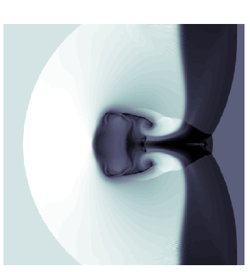
(a) (b)

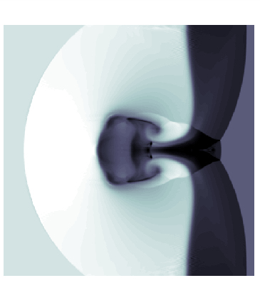
Figure 1: The 2.5D cloud-shock interaction problem. Shown here are the out-of-plane magnetic field at time $t=0.06$ as calculated on a 512$\times$512 mesh using (a) the scheme of [35] that only uses ${A}^{3}$, and (b) the proposed scheme using the full vector potential ${A}$.

6.2 Test cases in 3D

We present numerical results for three-dimensional versions of three classical MHD test problems:

1. Smooth Alfvén wave;

2. Rotated shock tube problem;

3. Orszag-Tang vortex; and

4. Cloud-shock interaction.

Two-dimensional versions of these problems have been studied by many authors, see for instance [35, 40].

Our test calculations will all be based on the splitting (77)–(79). We also carried out several tests with (74)–(76); however, we will not report those here. The two methods produced comparable results.

6.2.1 Smooth Alfvén wave problem

We first verify the order of convergence of the constrained transport method for a smooth circular polarized Alfvén wave that propagates in direction ${\bf n}=(\cos\phi\cos\theta,\sin\phi\cos\theta,\sin\theta)^{T}$ towards the origin. Here $\phi$ is an angle with respect to the $x$-axis in the $xy$-plane and $\theta$ is an angle with respect to the $xz$-plane. Initial values for the velocity and the magnetic field are specified in the direction ${\bf n}$ as well as the orthonormal directions ${\bf t}=(-\sin\phi,\cos\phi,0)^{T}$ and ${\bf r}=(-\cos\phi\sin\theta,-\sin\phi\sin\theta,\cos\theta)^{T}$:

$${\bf u}(0,{\bf x}) =u^{n}\,{\bf n}+u^{t}\,{\bf t}+u^{r}\,{\bf r},$$ (110)

$${\bf B}(0,{\bf x}) =B^{n}\,{\bf n}+B^{t}\,{\bf t}+B^{r}\,{\bf r},$$ (111)

where

$$u^{n} =0,\quad B^{n}=1,$$ (112)

$$u^{t} =B^{t}=0.1\sin(2\pi\,{\bf n}\cdot{\bf x}),$$ (113)

$$u^{r} =B^{r}=0.1\cos(2\pi\,{\bf n}\cdot{\bf x}).$$ (114)

The initial density and pressure are constant and set to

$$\rho(0,{\bf x})=1\qquad\text{and}\qquad p(0,{\bf x})=0.1,$$ (115)

respectively. This choice guarantees that the Alfvén wave speed is $|v_{A}|=B_{n}/\sqrt{\rho}=1$, which means that the flow agrees with the initial state whenever the time is an integer value. The computational domain is taken to be

$$\Omega=\left[0,\frac{1}{\cos\phi\cos\theta}\right]\times\left[0,\frac{1}{\sin\phi\cos\theta}\right]\times\left[0,\frac{1}{\sin\theta}\right],$$ (116)

with periodic boundary conditions imposed on the conserved variables in all three coordinate directions: $\left(\rho,\,\rho{\bf u},\,{\mathcal{E}},\,{\bf B}\right)$.

Our initial condition for the magnetic potential is

$${A}^{1}(0,{\bf x}) =z\left<B^{2}\right>-\frac{1}{20\pi}\sin\phi\sin(2\pi\,{\bf n}\cdot{\bf x}),$$ (117)

$${A}^{2}(0,{\bf x}) =x\left<B^{3}\right>+\frac{1}{20\pi}\cos\phi\sin(2\pi\,{\bf n}\cdot{\bf x}),$$ (118)

$${A}^{3}(0,{\bf x}) =y\left<B^{1}\right>+\frac{1}{20\pi\cos\theta}\cos(2\pi\,{\bf n}\cdot{\bf x}),$$ (119)

where $\left<{\bf B}\right>$ denotes the average magnetic field over the computational domain:

$$\left<{\bf B}\right>:=\frac{1}{|\Omega|}\iiint_{\Omega}{\bf B}(t,x,y,z)\,dx\,dy\,dz=\left(\cos\phi\cos\theta,\,\sin\phi\cos\theta,\,\sin\theta\right)^{T}.$$ (120)

We note that even though the magnetic field is time-dependent, its average, $\left<{\bf B}\right>$, is time-independent. Therefore, the magnetic potential consists of a linear (time-independent) and a periodic (time-dependent) part. Boundary conditions for the magnetic potential are handled by applying periodic boundary conditions on the periodic part and linear extrapolation for the linear part (linear extrapolation is exact in this case).

In Table 2 we show the results of a numerical convergence study in the three-dimensional case with $\theta=\phi=\tan^{-1}(0.5)\approx 26.5651^{\circ}$. These results confirm that our method is second order accurate.

Mesh	$L_{\infty}$ Error in $B^{1}$	$L_{\infty}$ Error in $B^{2}$	$L_{\infty}$ Error in $B^{3}$
$16\times 32\times 32$	$1.022\times 10^{-2}$	$2.787\times 10^{-2}$	$2.382\times 10^{-2}$
$32\times 64\times 64$	$2.577\times 10^{-3}$	$7.075\times 10^{-3}$	$6.101\times 10^{-3}$
$64\times 128\times 128$	$6.487\times 10^{-4}$	$1.782\times 10^{-3}$	$1.549\times 10^{-3}$
Order	1.990	1.989	1.978

Mesh	$L_{\infty}$ Error in ${A}^{1}$	$L_{\infty}$ Error in ${A}^{2}$	$L_{\infty}$ Error in ${A}^{3}$
$16\times 32\times 32$	$1.902\times 10^{-1}$	$1.460\times 10^{-1}$	$1.187\times 10^{-1}$
$32\times 64\times 64$	$4.816\times 10^{-2}$	$3.747\times 10^{-2}$	$2.995\times 10^{-2}$
$64\times 128\times 128$	$1.220\times 10^{-2}$	$9.528\times 10^{-3}$	$7.564\times 10^{-3}$
Order	1.981	1.975	1.985

Table 2: Error tables for the 3D Alfv$\acute{\text{e}}$n problem at time $t=1$. This table shows that all components of the magnetic field and all components of the magnetic potential converge at second order accuracy. The approximate order of accuracy is computed by taking the $\log_{2}$ of the ratio of the error on the $32\times 64\times 64$ mesh to the error on the $64\times 128\times 128$ mesh.

6.3 Rotated shock tube problem

We now consider the shock tube problem described in [27, 38]. In this test case a one-dimensional shock tube problem is computed in a three-dimensional domain. In order to define the problem, we consider a coordinate transformation of the form

$$\begin{bmatrix}\xi\\ \eta\\ \zeta\end{bmatrix}=\begin{bmatrix}\cos(\alpha)\cos(\beta)&\cos(\alpha)\sin(\beta)&\sin(\alpha)\\ -\sin(\beta)&\cos(\beta)&0\\ -\sin(\alpha)\cos(\beta)&-\sin(\alpha)\sin(\beta)&\cos(\alpha)\end{bmatrix}\begin{bmatrix}x\\ y\\ z\end{bmatrix},$$ (121)

which maps the Cartesian coordinates $(x,y,z)^{T}$ to the rotated coordinate system $(\xi,\eta,\zeta)^{T}$. Vectors transform as follows

$$\begin{bmatrix}B^{x}\\ B^{y}\\ B^{z}\end{bmatrix}=\begin{bmatrix}\cos(\alpha)\cos(\beta)&-\sin(\beta)&-\sin(\alpha)\cos(\beta)\\ \cos(\alpha)\sin(\beta)&\cos(\beta)&-\sin(\alpha)\sin(\beta)\\ \sin(\alpha)&0&\cos(\alpha)\end{bmatrix}\begin{bmatrix}B^{\xi}\\ B^{\eta}\\ B^{\zeta}\end{bmatrix}.$$ (122)

The Riemann initial data is taken to be

$$\begin{split}&\left(\rho,\,u^{\xi},\,u^{\eta},\,u^{\zeta},\,p,\,B^{\xi},\,B^{\eta},\,B^{\zeta}\right)(0,{\bf x})\\ &=\left\{\begin{array}[]{l c c}\Bigl{(}1.08,\,1.2,\,0.01,\,0.5,\,0.95,\,\frac{2}{\sqrt{4\pi}},\,\frac{3.6}{\sqrt{4\pi}},\,\frac{2}{\sqrt{4\pi}}\Bigr{)}&\text{if}&\xi<0,\\ \Bigl{(}1,\,0,\,0,\,0,\,1,\,\frac{2}{\sqrt{4\pi}},\,\frac{4}{\sqrt{4\pi}},\,\frac{2}{\sqrt{4\pi}}\Bigr{)}&\text{if}&\xi\geq 0,\end{array}\right.\end{split}$$ (123)

where the velocity vector and the magnetic field are given in the rotated coordinate frame. As the initial condition for the magnetic potential (in the rotated coordinate frame) we use

$$\left({{A}}^{\xi},\,{{A}}^{\eta},\,{{A}}^{\zeta}\right)(0,{\bf x})=\left(0,\,\xi B^{\zeta},\,\eta B^{\xi}-\xi B^{\eta}\right).$$ (124)

The solution of the Riemann problem at later times remains a function of $\xi$. This fact is used to extend the computed values to ghost cell values. The computational domain is $\Omega=[-0.75,0.75]\times[0,0.015625]\times[0,0.015625]$, which is discretized using $768\times 8\times 8$ grid cells. By using $\alpha=\tan^{-1}(0.5)$ and $\beta=\tan^{-1}(0.25\cos\alpha)$, we obtain simple formulas for the extension of the numerical solution to the ghost cells.To define ghost cell values in the Cartesian $y$-direction, we can for instance use the relation $q(i,j,k)=q(i+1,j-2,k)$. In the $z$-direction we can use $q(i,j,k)=q(i+1,j,k-4)$. The ghost cell values in the $x$-direction were computed via extrapolation. We present numerical results at time $t=0.2$ as scatter plots of the three-dimensional solution plotted as a function of $\xi$.

As already documented by other authors, we also observe some oscillations in particular in the $B^{\xi}$ component of the magnetic field. These oscillations do not appear if the shock tube initial data are aligned with the mesh. In Figure 2 we show approximations of the solution at time $t=0.2$. These plots are scatterplots, where the output of the three-dimensional computation is plotted as a function of $\xi$. The solid line in these plots is obtained by computing solutions of the one-dimensional Riemann problem on a very fine mesh (using $10^{4}$ grid cells). The computation was performed using the minmod limiter and the diffusive limiter with $\nu=0.05$. As expected, with a less diffusive limiter the amplitude of the oscillations becomes stronger, by increasing $\nu$, the amplitude of the oscillations becomes weaker.

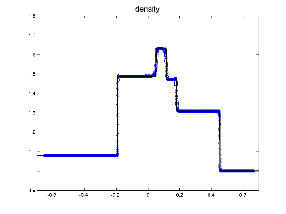
(a) (b)

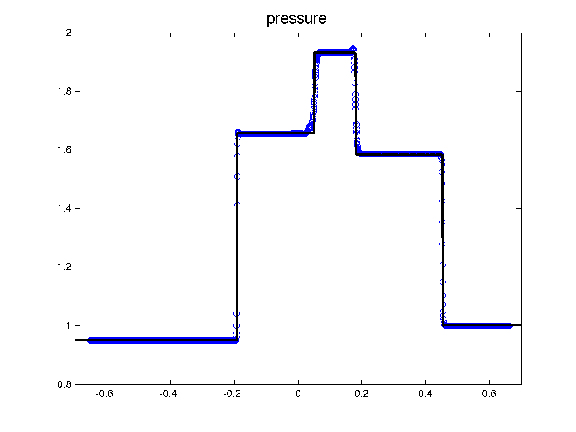
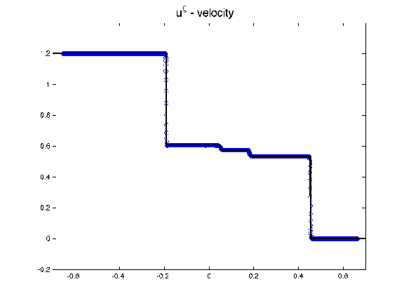
(c) (d)

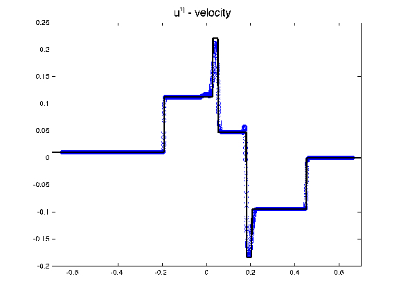
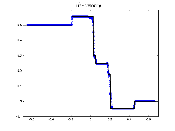
(e) (f)

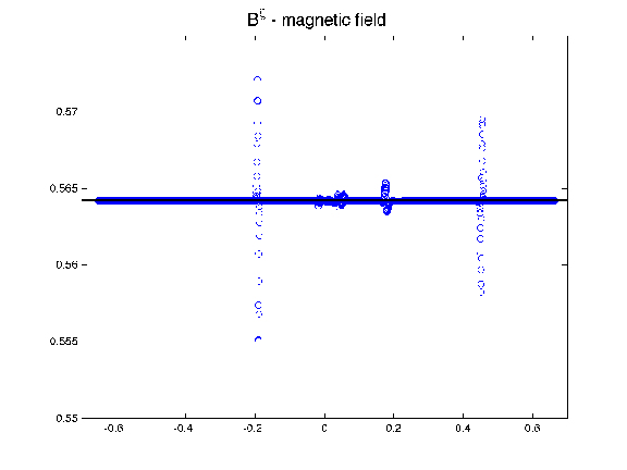
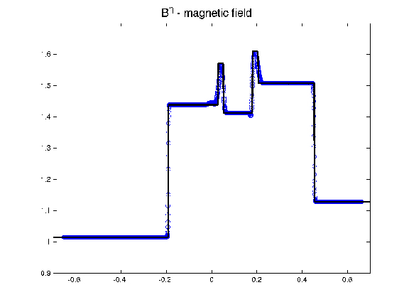
(g) (h)

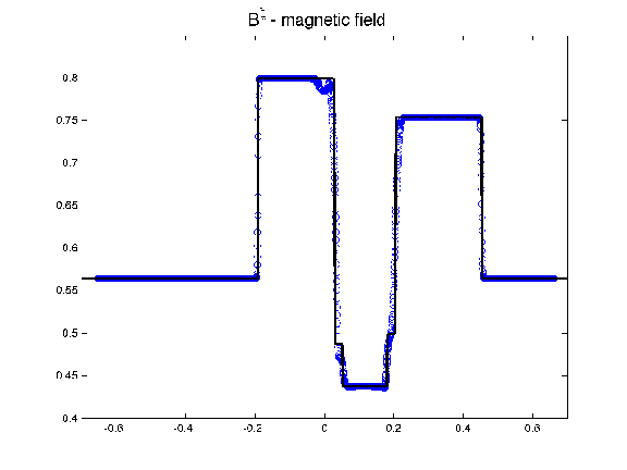
Figure 2: The rotated Riemann problem. Scatterplots of various components of solution at time $t=0.2$ using the constrained transport algorithm. The solid line in each panel is a highly-resolved 1D simulation.

6.3.1 Orszag-Tang vortex

Our next test problem is the Orszag-Tang vortex problem. This is a standard test case for the two-dimensional MHD equations. Here we add a small perturbation to the initial velocity field that depends on the vertical direction.

The initial condition is

$$\rho(0,{\bf x}) =\gamma^{2},\quad p(0,{\bf x})=\gamma,$$ (125)

$${\bf u}(0,{\bf x}) =\Bigl{(}-(1+\varepsilon\sin z)\sin y,\,(1+\varepsilon\sin z)\sin x,\,\varepsilon\sin(z)\Bigr{)}^{T},$$ (126)

$${\bf B}(0,{\bf x}) =\Bigl{(}-\sin y,\,\sin(2x),\,0\Bigr{)}^{T}.$$ (127)

Here we used $\varepsilon=0.2$. The initial condition for the magnetic potential is

$${\bf A}(0,{\bf x})=\Bigl{(}0,\,0,\,\cos y+\cos(2x)\Bigr{)}^{T}.$$ (128)

The computational domain is a cube with side length $2\pi$. Periodicity is imposed in all three directions.

In Figures 3-6 we show a sequence of schlieren plots of the pressure for several slices of data in the $xy$-plane for $z=\pi/2,\,\pi,\,3\pi/2$. Those computations have been performed with the high-resolution constrained transport method with monotonized central limiter and the diffusive limiter using $\nu=0.05$. In Figures 7, 8 we show schlieren plots of pressure in the $xy$-plane for $z=\pi$ at different times.

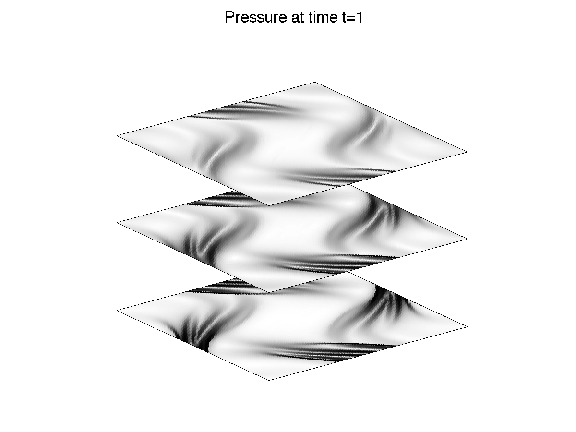
Figure 3: The 3D Orszag-Tang problem. Shown in this figure are schlieren slices of pressure at time $t=1$ and at various $z$ values ($z=\pi/2,\,\pi,\,3\pi/2$). This solution was computed on a mesh with $150\times 150\times 150$ grid cells.

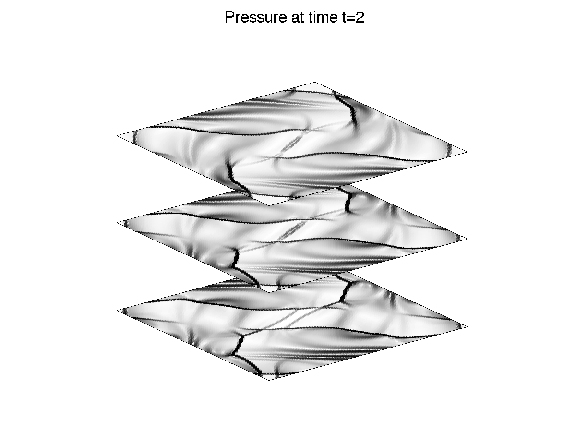
Figure 4: The 3D Orszag-Tang problem. Shown in this figure are schlieren slices of pressure at time $t=2$ and at various $z$ values ($z=\pi/2,\,\pi,\,3\pi/2$). This solution was computed on a mesh with $150\times 150\times 150$ grid cells.

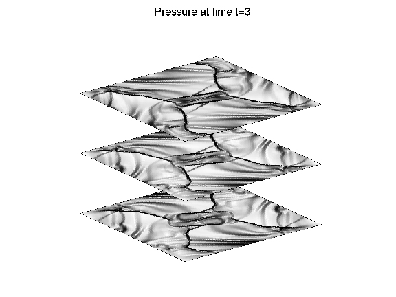
Figure 5: The 3D Orszag-Tang problem. Shown in this figure are schlieren slices of pressure at time $t=3$ and at various $z$ values ($z=\pi/2,\,\pi,\,3\pi/2$). This solution was computed on a mesh with $150\times 150\times 150$ grid cells.

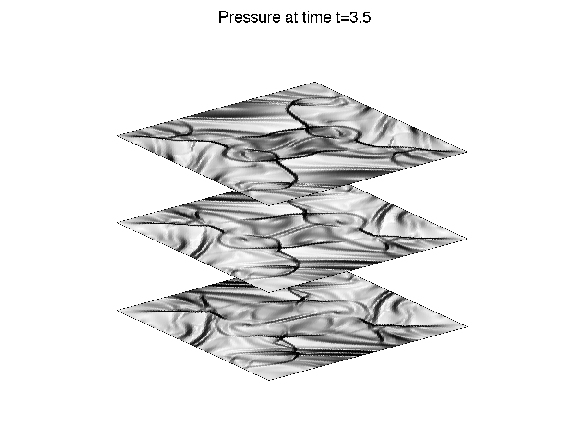
Figure 6: The 3D Orszag-Tang problem. Shown in this figure are schlieren slices of pressure at time $t=3.5$ and at various $z$ values ($z=\pi/2,\,\pi,\,3\pi/2$). This solution was computed on a mesh with $150\times 150\times 150$ grid cells.

(a)

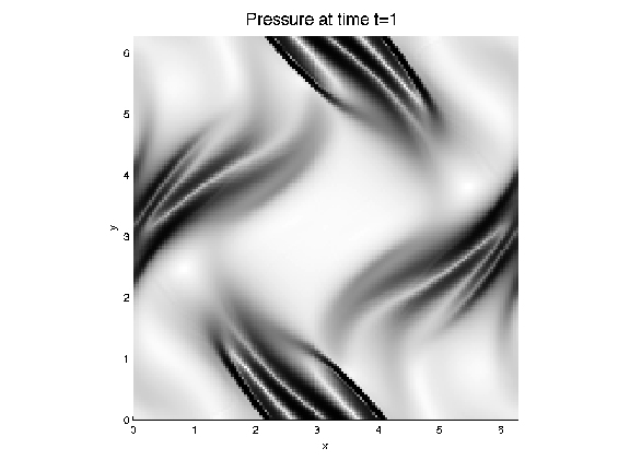
(b)

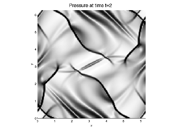
Figure 7: The 3D Orszag-Tang problem. Schlieren plots of pressure at time (a) $t=1$ and (b) $t=2$ computed on a mesh with $150\times 150\times 150$ grid cells. Slices of the solution at $z=\pi$ in the $xy$-plane are shown.

(a)

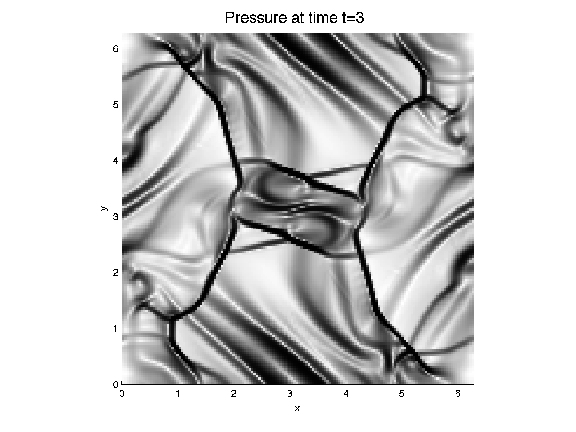
(b)

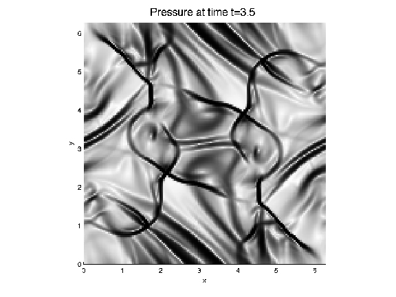
Figure 8: The 3D Orszag-Tang vortex problem. Shown in these panels are schlieren plots of pressure in the $xy$-plane at (a) time $t=3$ and $z=\pi$ and (b) $t=3.5$ and $z=\pi$. These solutions were computed on a mesh with $150\times 150\times 150$ grid cells.

6.3.2 Cloud-shock interaction problem

Finally we consider the cloud-shock interaction problem. The initial conditions consist of a shock that is initially located at $x=0.05$:

$$\begin{split}&\left(\rho,\,u^{1},\,u^{2},\,u^{3},\,p,\,B^{1},\,B^{2},\,B^{3}\right)(0,{\bf x})\\ &=\biggl{\{}\begin{array}[]{l c c}\left(3.86859,\,11.2536,\,0,\,0,\,167.345,\,0,\,2.1826182,\,-2.1826182\right)&\text{if}&x<0.05,\\ \left(1,\,0,\,0,\,0,\,1,\,0,\,0.56418958,\,0.56418958\right)&\text{if}&x\geq 0.05,\end{array}\end{split}$$ (129)

and a spherical cloud of density $\rho=10$ with radius $r=0.15$ and centered at $(0.25,0.5,0.5)$. The cloud is in hydrostatic equilibrium with the fluid to the right of the shock. The initial condition for the magnetic potential is

$${\bf A}(0,{\bf x})=\left\{\begin{array}[]{l c c}\left(2.1826182\,y,\,0,\,-2.1826182\,(x-0.05)\right)^{T}&\text{if}&x<0.05,\\ \left(-0.56418958\,y,\,0,\,0.56418956\,(x-0.05)\right)^{T}&\text{if}&x\geq 0.05.\end{array}\right.$$ (130)

This test problem can be computed on the unit cube with inflow boundary conditions on the left side and outflow conditions on all other sides. Instead we make use of the symmetry of the problem and compute the problem only in a quarter of the full domain, i.e. in $[0,1]\times[0.5,1]\times[0.5,1]$ and impose reflecting boundary conditions at the lower boundary in the $y$ and $z$-directions. For the conserved quantities, the reflecting boundary condition is implemented in the standard way, i.e., by copying the values of the conserved quantities from the first grid cells of the flow domain to the ghost cells. The normal momentum component in the ghost cells is negated. The components of the magnetic potential are linearly extrapolated to the ghost cells.

In Figures 9 and 10, we show a sequence of schlieren plots of the density in the $xy$-plane for $z=0.5$ and the $xz$-plane for $y=0.5$. The three-dimensional radial symmetric solution structure compares well with previously shown two-dimensional computations. In Figures 11 and 12 we show the schlieren plots of density in the $xz$-plane. Here the diffusive limiter described in §5.2 was used with $\nu=0.02$.

(a)

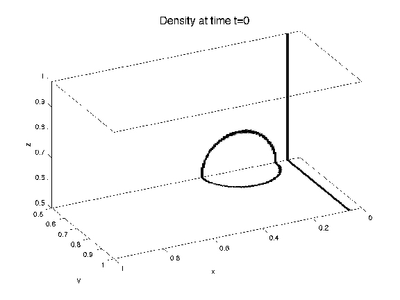
(b)

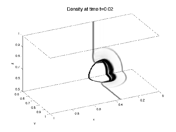
Figure 9: The 3D cloud-shock interaction problem. Schlieren plots of density for the problem using a mesh with $200\times 100\times 100$ grid cells at time (a) $t=0$ and (b) $t=0.02$. Shown here is the solution in two selected orthogonal planes.

(a)

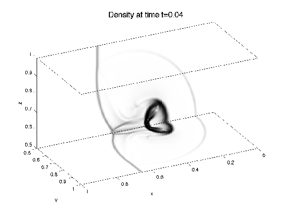
(b)

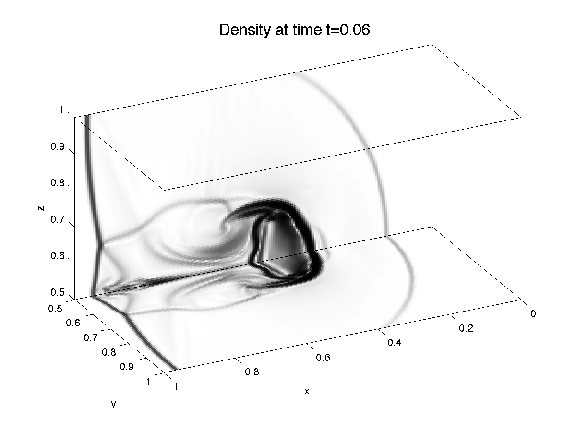
Figure 10: The 3D cloud-shock interaction problem. Schlieren plots of density using a mesh with $200\times 100\times 100$ grid cells at time (a) $t=0.04$ and (b) $t=0.06$. Shown here is the solution in two selected orthogonal planes.

(a)

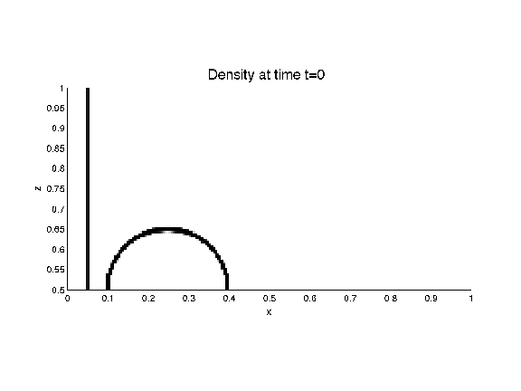
(b)

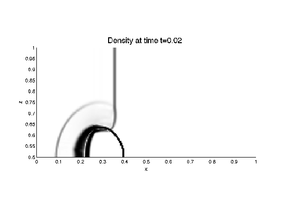
Figure 11: The 3D cloud-shock interaction problem. Sequence of schlieren plots of density in the $xz$-plane for $y=0.5$ at time (a) $t=0$ and (b) $t=0.02$.

(a)

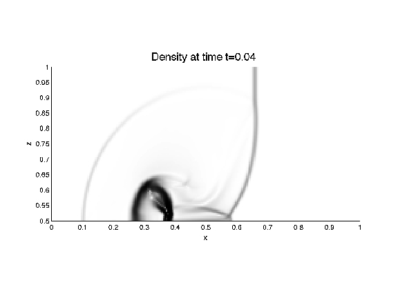
(b)

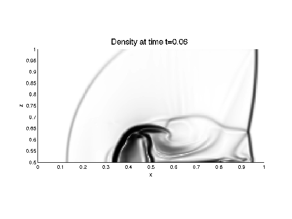
Figure 12: The 3D cloud-shock interaction problem. Sequence of schlieren plots of density in the $xz$-plane for $y=0.5$ at time (a) $t=0.04$ and (b) $t=0.06$.

7 Conclusions

We have presented a new constrained transport method for the three-dimensional MHD equations. Depending on the gauge condition, we discussed different possible evolution equations for the magnetic potential. All of these gauge conditions implicate some difficulties for the discretization. The condition used here leads to a weakly hyperbolic system for the evolution of the magnetic potential. We discretized this system with a splitting approach. For the MHD equations we used a wave propagation method. Several numerical tests confirm the robustness and accuracy of the resulting constrained transport scheme.

Our method is fully explicit, as well as fully unstaggered, and therefore well-suited for adaptive mesh refinement and parallelization. These generalizations will be the focus of future work.

Acknowledgements. The authors would like to thank Prof. Dr. Rainer Grauer from the Ruhr-Universität-Bochum for several useful discussions, as well as the anonymous reviewers for their valuable comments. This work was supported in part by NSF grants DMS-0711885 and DMS-1016202 and by the DFG through FOR1048.

References

- [1] D.S. Bale, R.J. LeVeque, S. Mitran, and J.A. Rossmanith. A wave propagation method for conservation laws and balance laws with spatially varying flux functions. SIAM J. Sci. Comp., 24:955–978, 2003.
- [2] D.S. Balsara. Second-order-accurate schemes for magnetohydrodynamics with divergence-free reconstruction. Astrophys. J. Suppl., 151:149–184, 2004.
- [3] D.S. Balsara and J. Kim. A comparison between divergence-cleaning and staggered-mesh formulations for numerical magnetohydrodynamics. Astrophys. J., 602:1079—1090, 2004.
- [4] D.S. Balsara and D. Spicer. A staggered mesh algorithm using high order Godunov fluxes to ensure solenoidal magnetic fields in magnetohydrodynamic simulations. J. Comp. Phys., 149(2):270–292, 1999.
- [5] T.J. Barth. On the role of involutions in the discontinuous Galerkin discretization of Maxwell and magnetohydrodynamic systems. In IMA Volume on Compatible Spatial Discretizations, volume 142. Springer-Verlag, 2005.
- [6] J.U. Brackbill and D.C. Barnes. The effect of nonzero on the numerical solution of the magnetohydrodynamic equations. J. Comp. Phys., 35:426–430, 1980.
- [7] P. Cargo and G. Gallice. Roe matrices for ideal MHD and systematic construction of Roe matrices for systems of conservation laws. J. Comp. Phys., 136:446–466, 1997.
- [8] F.F. Chen. Introduction to Plasma Physics and Controlled Fusion. Plenum Press, 1984.
- [9] P. Colella. Multidimensional upwind methods for hyperbolic conservation laws. J. Comp. Phys., 87:171–200, 1990.
- [10] C. Dafermos. Hyperbolic Conservation Laws in Continuum Physics. Springer, 2010.
- [11] W. Dai and P.R. Woodward. A simple finite difference scheme for multidimensional magnetohydrodynamic equations. J. Comp. Phys., 142(2):331–369, 1998.
- [12] A. Dedner, F. Kemm, D. Kröner, C.-D. Munz, T. Schnitzer, and M. Wesenberg. Hyperbolic divergence cleaning for the MHD equations. J. Comp. Phys., 175:645–673, 2002.
- [13] E.A. Dorfi. Numerical methods for astrophysical plasmas. Comp. Phys. Comm., 43:1–15, 1986.
- [14] C. Evans and J.F. Hawley. Simulation of magnetohydrodynamic flow: A constrained transport method. Astrophys. J., 332:659–677, 1988.
- [15] M. Fey and M. Torrilhon. A constrained transport upwind scheme for divergence-free advection. In T.Y. Hou and E. Tadmor, editors, Hyperbolic Problems: Theory, Numerics, and Applications, pages 529–538. Springer, 2003.
- [16] T.A. Gardiner and J.M. Stone. An unsplit Godunov method for ideal MHD via constrained transport. J. Comp. Phys., 205:509–539, 2005.
- [17] T.A. Gardiner and J.M. Stone. An unsplit Godunov method for ideal MHD via constrained transport in three dimensions. J. Comp. Phys., 227:4123–4141, 2008.
- [18] S.K. Godunov. Symmetric form of the magnetohydrodynamic equations. Numerical Methods for Mechanics of Continuum Medium, 1:26–34, 1972.
- [19] T.I. Gombosi. Physics of the Space Environment. Cambridge University Press, 1998.
- [20] A. Harten. High resolution schemes for hyperbolic conservation laws. J. Comp. Phys., 49:357–393, 1983.
- [21] J.O. Langseth and R.J. LeVeque. A wave propagation method for three-dimensional hyperbolic conservation laws. J. Comp. Phys., 165:126–166, 2000.
-
[22]
R.J. LeVeque.
The clawpack software package.
Available from
http://www.amath.washington.edu/claw. - [23] R.J. LeVeque. Wave propagation algorithms for multi-dimensional hyperbolic systems. J. Comp. Phys., 131:327–335, 1997.
- [24] R.J. LeVeque. Finite Volume Methods for Hyperbolic Problems. Cambridge University Press, 2002.
- [25] P. Londrillo and L. Del Zanna. High-order upwind schemes for multidimensional magnetohydrodynamics. Astrophys. J., 530:508–524, 2000.
- [26] P. Londrillo and L. Del Zanna. On the divergence-free condition in godunov-type schemes for ideal magnetohydrodynamics: the upwind constrained transport method. J. Comp. Phys., 195:17–48, 2004.
- [27] A. Mignone and P. Tzeferacos. A second-order unsplit Godunov scheme for cell-centered MHD: The CTU-GLM scheme. J. Comp. Phys., 229:2117–2138, 2010.
- [28] G.K. Parks. Physics of Space Plasmas: An Introduction. Addison-Wesley, 1991.
- [29] P.-O. Persson and J. Perraire. Sub-cell shock capturing for discontinuous Galerkin methods. AIAA, 2006.
- [30] E. Poisson. A Relativist’s Toolkit: The Mathematics of Black-Hole Mechanics. Cambridge University Press, 2004.
- [31] K.G. Powell. An approximate Riemann solver for magnetohydrodynamics (that works in more than one dimension). Technical Report 94-24, ICASE, Langley, VA, 1994.
- [32] K.G. Powell, P.L. Roe, T.J. Linde, T.I. Gombosi, and D.L. De Zeeuw. A solution-adaptive upwind scheme for ideal magnetohydrodynamics. J. Comp. Phys., 154:284–309, 1999.
- [33] P.L. Roe and D. Balsara. Notes on the eigensystem of magnetohydrodynamics. SIAM Appl. Math., 56:57–67, 1996.
-
[34]
J.A. Rossmanith.
The mhdclaw software package.
Available from
http://www.math.wisc.edu/rossmani/MHDCLAW. - [35] J.A. Rossmanith. An unstaggered, high-resolution constrained transport method for magnetohydrodynamic flows. SIAM J. Sci. Comp., 28:1766–1797, 2006.
- [36] D.S. Ryu, F. Miniati, T.W. Jones, and A. Frank. A divergence-free upwind code for multidimensional magnetohydrodynamic flows. Astrophys. J., 509(1):244–255, 1998.
- [37] H. De Sterck. Multi-dimensional upwind constrained transport on unstructured grids for “shallow water” magnetohydrodynamics. In Proceedings of the 15th AIAA Computational Fluid Dynamics Conference, Anaheim, California, page 2623. AIAA, 2001.
- [38] J.M. Stone and T. Gardiner. A simple unsplit Godunov method for multidimensional MHD. New Astronomy, 14:139–148, 2009.
- [39] P.K. Sweby. High resolution schemes using flux limiters for hyperbolic conservation laws. SIAM J. Num. Anal., 21:995–1011, 1984.
- [40] G. Tth. The constraint in shock-capturing magnetohydrodynamics codes. J. Comp. Phys., 161:605–652, 2000.
- [41] G. Tth. Conservative and orthogonal discretization for the Lorentz force. J. Comp. Phys., 182:346–354, 2002.
- [42] E. Tadmor. Entropy stability theory for difference approximations of nonlinear conservation laws and related time-dependent problems. Acta Numerica, 12:451–512, 2003.
- [43] B. van Leer. Towards the ultimate conservative difference scheme II. Monotonicity and conservation combined in a second order scheme. J. Comp. Phys., 14:361–370, 1974.
- [44] B. van Leer. Flux-vector splitting for the Euler equations. In E. Krause, editor, Lecture Notes in Physics, volume 170. Springer-Verlag, 1982.
- [45] M. Wesenberg. Efficient MHD Riemann solvers for simulations on unstructured triangular grids. J. Numer. Math., 10:37–71, 2002.
- [46] J.R. Wilson. Some magnetic effects in stellar collapse and accretion. Ann. N.Y. Acad. Sci., 262:123–132, 1975.
- [47] K. Yee. Numerical solutions of initial boundary value problems involving Maxwell’s equations in isotropic media. IEEE Transactions on Antennas and Propagation, AP-14:302–307, 1966.