The next-to-leading-order QCD correction to inclusive $J/\psi(\Upsilon)$ production in Z⁰ decay

Abstract

In this paper, we study the $J/\psi(\Upsilon)$ production in Z boson decay in color-singlet model(CSM). We calculate the next-to-leading-order (NLO) QCD correction to $Z\to Quarkonium+Q\bar{Q}$, the dominant contribution in the CSM, with the vector and axial-vector parts in $ZQ\bar{Q}$ vertex being treated separately. The results show that the vector and axial-vector parts have the same K factor (the ratio of NLO result to leading-order result) 1.13 with the renormalization scale $\mu$=2$m_{c}$ and $m_{c}=1.5GeV$, and the K factor falls to 0.918 when applying the Brodsky, Lepage, and Mackenzie(BLM) renormalization scale scheme with obtained $\mu_{BLM}=2.28GeV$ and $m_{c}=1.5$GeV. By including the contributions from the next-dominant ones, the photon and gluon fragmentation processes, the branching ratio for $Z\to J/\psi_{prompt}+X$ is $(7.3\sim 10.0)\times 10^{-5}$ with the uncertainty consideration for the renormalization scale and Charm quark mass. The results are about half of the central value of the experimental measurement 2.1$\times 10^{-4}$. Furthermore, the $J/\psi$ energy distribution in our calculation is not well consistent with the experimental data. Therefore, even at QCD NLO, the contribution to $Z\to J/\psi_{prompt}+X$ from the CSM can not fully account for the experimental measurement. And there should be contributions from other mechanisms, such as the color-octet(COM) contributions. We define $R_{c\bar{c}}=\frac{\Gamma(Z\to J/\psi c\bar{c}X)}{\Gamma(Z\to J/\psi X)}$ and obtain $R_{cc}=0.84$ for only CSM contribution and $R_{cc}=0.49$ for COM and CSM contributions together. Then $R_{cc}$ measurement could be used to clarify the COM contributions.

I I. Introduction

Heavy Quarkonium is an ideal system being used to study the perturbative and non-perturbative aspects of QCD. Firstly, the heavy quark mass sets a large scale for perturbative calculation. Secondly, the dileptonic decay of heavy quarkonium makes the identification and measurement efficient. In 1995, the non-relativistic QCD(NRQCD), a rigorous effective theory in describing the production and decay of heavy quarkonium, was proposed Bodwin:1994jh , and it makes the color-singlet model(CSM) Einhorn:1975ua be its leading-order approximation in $v$ (the velocity between heavy quark and anti-quark in the meson rest frame). More details on NRQCD and heavy quarkonium physics can be found in reference Brambilla:2004wf .

In recent years, there are many works on the next-to-leading-order(NLO) QCD correction for heavy quarkonium productions. To explain the experimental measurement Abe:2001za ; Aubert:2005tj of $J/\psi$ production at the B factories, a series of calculations Zhang:2005cha ; Gong:2009ng have been performed and revealed that the NLO QCD corrections can change the leading-order(LO) theoretical predictions considerably and the NLO results in CSM give the main contribution to the related processes. Together with the relativistic correction Bodwin:2006ke , it seems that all the experimental data for $J/\psi$ production at the B factories could be understood. For $J/\psi$ production in the hadron colliders, there are obviously progress in the theoretical calculation. The NLO QCD correction to the CSM processesCampbell:2007ws ; Gong:2008sn greatly enhanced the $p_{t}$ (transverse momentum of $J/\psi$) distribution of $J/\psi$ production at large $p_{t}$ region, and the $p_{t}$ distribution of $J/\psi$ polarization is drastically changed from mostly transverse polarization at LO into mostly longitudinal polarization at NLO Gong:2008sn . It is found that the NLO QCD correction to $J/\psi$ production for color-octet (COM) parts is quite small, about 10 percent Gong:2008ft . Even including all these progresses, we still can not obtain an satisfactory explanation on both the $p_{t}$ distribution of the production and polarization for $J/\psi$ hadroproduction. The partial next-to-next-to-leading-order(NNLO) calculations for $\Upsilon$ and $J/\psi$ hadroproduction show that the uncertainty form QCD higher order correction Artoisenet:2008fc is much bigger, but still can not cover the $J/\psi$ or $\Upsilon$ polarization measurement. Recent studies reveal that the NLO QCD correction also plays an important role on $J/\psi$ production at RHIC Brodsky:2009cf and the hadroproduction of $\chi_{c}$ Ma:2010vd . The $J/\psi$ photoproduction once was considered as an positive example with the $p_{t}$ and $z$ distribution well described by the NLO calculations in CSM Kramer:1995nb . But either the $p_{t}$ distribution of the production or polarization for $J/\psi$ can not be well described by the recent NLO calculations in CSM Artoisenet:2009xh . It seems that the complete calculation at NLO in COM  Butenschoen:2009zy can account for the experimental measurements on the $p_{t}$ distribution. But the complete calculation on $J/\psi$ polarization at NLO in COM is a real challenge.

With both the successful and unsuccessful aspects for theoretical progress in heavy quarkonium production, it is worthwhile to study more cases in detail. Such as $J/\psi$ production associated with photon Li:2008ym , QED contributions in $J/\psi$ hadroproduction He:2009cq , inclusive $J/\psi$ production from $\Upsilon$ decay He:2009by and $J/\psi$ production from $Z$ decay. Heavy quarkonium production in Z decay has been widely studied in the CSM and COM at LO Guberina:1980dc ; Cheung:1995ka ; Baek:1996kq ; Fleming:1993fq , and the measurement at the LEP by L3 Collaboration gives the branching ratio as Acciarri:1998iy

$$Br(Z\to J/\psi_{prompt}+X)$$

$$=(2.1\pm 0.6(stat.)\pm 0.4(sys.)^{+0.4}_{-0.2}(theo.))\times 10^{-4},$$ (1)

$$Br(Z\to\Upsilon(1S)+X)<4.4\times 10^{-5}.$$ (2)

Theoretical investigation on this process indicates that even the dominant channel $Z\to J/\psi+c+\bar{c}$ in all the CSM ones at LO only gives the 1/3 prediction to the total branching ratio of the experimental measurement. Including the contribution of gluon fragmentation process in the COM can enhance the theoretical results about 3 times Cheung:1995ka . This once is an evidence for the effect of the COM. It also have been studied in color-evaporation model(CEM) in reference Gregores:1996ek and obtained consistent results with the experimental data. But the CEM always gives unpolarized $J/\psi$ in conflict with experimental measurements. By resuming the large logarithm from the large difference of $J/\psi$ and Z mass, the COM prediction on $J/\psi$ energy distribution($d\Gamma/dz$ with $z$=2$E_{J/\psi}/M_{z}$) is roughly consist with the data Boyd:1998km . Considering the larger impact of the NLO QCD corrections to the production of heavy quarkonium, it is necessary to investigate the NLO QCD correction to $Z\to J/\psi+c\bar{c}+X$. In this paper, we calculate the NLO QCD correction to $Z\to J/\psi+c\bar{c}+X$, and also include the contributions from the gluon and photon fragmentation processes as well with only the CSM in consideration. The study could provide more insight to the effect of color-octet mechanism and put more constrains on the value of color-octet matrix elements.

This paper is organized as follows. In Sec. II, we study the NLO QCD correction to the heavy quark association process with different schemes on the choice of renormalization scale. In Sec. III, we investigated dominant fragmentation processes and give the total results on prompt $J/\psi$ production in Z decay. In Sec. IV, the summary and conclusion are presented.

II II. The heavy quark association process

For the calculation on $Z\to J/\psi+c\bar{c}+X$ at NLO, there are virtual and real  correction parts as

$$Z\to J/\psi+c+\bar{c}$$ (3)

$$Z\to J/\psi+c+\bar{c}+g.$$ (4)

There are vector and axial-vector parts in the coupling of Z boson to fermions, but the interference between them does not contribute in our calculation. Therefore, we study them separately. There are 4 Feynman diagrams for both parts at LO, 80 for the vector part and 76 for the axial-vector part at NLO. The typical diagrams are presented in Fig. 1.

Figure 1: Typical Feynman diagrams for $J/\psi+c\bar{c}+X$ production in Z decay. B is the Born diagram. CV1$\sim$CV5 represent the counterterm diagrams and corresponding loop diagrams. V1$\sim$V7 represent the box and the anomalous triangle diagrams. R1 and R2 are the real parts.

The dimensional regularization is used to regulate the the ultraviolet (UV) and infrared (IR) divergence, and the Coulomb singularity is regulated by introducing a small relative velocity between quark pair in the quarkonium and absorbed into the wave function of quarkonium. In calculating the axial-vector part, we have to face the $\gamma_{5}$ problem. The structure of all the amplitude squared diagrams could be classified into four cases shown in Fig. 2.

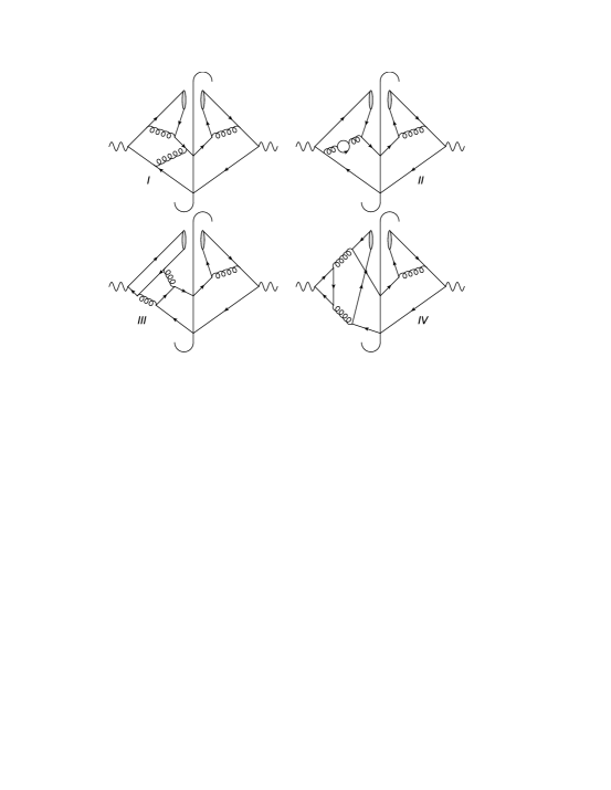
Figure 2: The typical amplitude squared diagrams for $J/\psi+c\bar{c}+X$ production in Z decay.

Case 1. There are only one fermion-loop and two $\gamma_{5}$ matrices appear in it. Then $\gamma_{5}$s can be moved together and give an identity matrix by $\gamma^{2}_{5}=1$.

Case 2. There are two fermion-loops and the two $\gamma_{5}$ matrices appear in one of them. It is the same as case 1.

Case 3. There are two fermion-loops. Each of them has a $\gamma_{5}$. Because there are no UV and IR divergences in the loops, the dimension can be set as 4 safely.

Case 4. The only special case are the two triangle anomalous diagrams. In this case we use the scheme described in reference Korner:1991sx to handle it, which fixes the starting point to write down all the amplitude and abandon the cyclicity in calculating the trace of the fermion-loop with odd number of $\gamma_{5}$. This two triangle anomalous diagrams will not contribute at all according to Yang’s theorem Yang:1950rg when the two gluon lines are on mass-shell, but will contribute in our case since the two connected gluons are off mass-shell.

The on-mass-shell (OS) scheme is used to define the renormalization constants $Z_{m}$, $Z_{2}$ and $Z_{3}$, which correspond to charm quark mass $m_{c}$, charm field $\psi_{c}$, and gluon field $A^{a}_{\mu}$ while $Z_{g}$ for the QCD gauge coupling $\alpha_{s}$ is defined in the modified-minimal-subtraction($\overline{\mathrm{MS}}$) scheme:

$$\delta Z_{m}^{\mathrm{OS}} = -3C_{F}\dfrac{\alpha_{s}}{4\pi}[\dfrac{1}{\epsilon_{UV}}-\gamma_{E}+\ln\dfrac{4\pi\mu^{2}}{m_{c}^{2}}+\frac{4}{3}],$$

$$\delta Z_{2}^{\mathrm{OS}} = -C_{F}\dfrac{\alpha_{s}}{4\pi}\biggl{[}\dfrac{1}{\epsilon_{UV}}+\dfrac{2}{\epsilon_{IR}}-3\gamma_{E}+3\ln\dfrac{4\pi\mu^{2}}{m_{c}^{2}}+4\biggr{]},$$

$$\delta Z_{3}^{\mathrm{OS}} = \dfrac{\alpha_{s}}{4\pi}\biggl{[}(\beta^{\prime}_{0}-2C_{A})(\dfrac{1}{\epsilon_{UV}}-\dfrac{1}{\epsilon_{IR}})$$

$$-\dfrac{4}{3}T_{F}(\dfrac{1}{\epsilon_{UV}}-\gamma_{E}+\ln\dfrac{4\pi\mu^{2}}{m_{c}^{2}})\biggr{]},$$

$$\delta Z_{g}^{\overline{\mathrm{MS}}} = -\dfrac{\beta_{0}}{2}\dfrac{\alpha_{s}}{4\pi}[\dfrac{1}{\epsilon_{UV}}-\gamma_{E}+\ln(4\pi)].$$ (5)

where $\mu$ is the renormalization scale, $\gamma_{E}$ is Euler’s constant, $\beta_{0}=\frac{11}{3}C_{A}-\frac{4}{3}T_{F}n_{f}$ is the one-loop coefficient of the QCD beta function and $n_{f}$ is the number of active quark flavors. There are three massless light quarks $u,d,s$, and heavy quark $c$, so $n_{f}$=4. In $SU(3)_{c}$, color factors are given by $T_{F}=\frac{1}{2},C_{F}=\frac{4}{3},C_{A}=3$. And $\beta^{\prime}_{0}\equiv\beta_{0}+(4/3)T_{F}=(11/3)C_{A}-(4/3)T_{F}n_{lf}$ where $n_{lf}\equiv n_{f}-1=3$ is the number of light quarks flavors. Actually in the NLO total amplitude level, the terms proportion to $\delta{Z_{3}}^{\mathrm{OS}}$ cancel each other, thus the result is independent of renormalization scheme of the gluon field. The above renormalization scheme and constant are similar to those in reference Gong:2007db . The bottom quark should be considered for the calculation of $\Upsilon$ production.

We use the Feynman Diagram Calculation(FDC) package Wang:2004du to generate Feynman diagram and amplitude, to do the tensor reduction and scalar integration, and to give the FORTRAN code for numerical calculation finally. Because there are some large numbers generated in the program, the quadruple precision FORTRAN source is used.

The leptonic width of $J/\psi(\Upsilon)$ is used to extract their wave functions at origin $R_{s}^{J/\psi(\Upsilon)}$, which is

$$\Gamma_{ee}=(1-\frac{16\alpha_{s}}{3\pi})\frac{4\alpha^{2}e_{c(b)}^{2}}{M_{J/\psi(\Upsilon)}^{2}}|R_{s}^{J/\psi(\Upsilon)}|^{2}.$$

Here the values of the parameters are chosen as $\Gamma_{ee}^{J/\psi}=5.55$keV, $\Gamma_{ee}^{\Upsilon}=1.34$keV Amsler:2008zz , $\alpha$=1/137 and $\alpha_{s}=\alpha_{s}^{2loop}(2m_{Q})$. The one-loop and two-loop running program of CTEQ6 are used to fix the LO and NLO values of $\alpha_{s}$. The LO wave functions of heavy quarkonium are used to obtain the LO results in Fig. 3, 4, 5 and  6. In the following calculation, $\alpha=1/128$ is used, and the central value of heavy quark mass is chosen as $m_{c}$=1.5GeV ($m_{b}$=4.75GeV). We also use $m_{c}$=1.4,1.6 GeV ($m_{b}$=4.65, 4.85 GeV) for uncertainty estimate. The default choice of renormalization scale is 2$m_{c}$(2$m_{b}$) for $J/\psi$ ($\Upsilon$).

The LO and NLO partial decay width of $Z\to J/\psi+c\bar{c}+X$ are presented in Table  1. The difference between our LO results and the other LO results in literature is mainly due to the different choice of the wave functions at origin. The QCD correction enhance the partial decay width about 13$\%$ for both the vector part and the axial-vector part when the same wave function at origin is used. This may provide a hint that the picture of heavy quark fragmentation into quarkonium works at these energy scale at NLO. It can also be seen that the K factors are insensitive to the variance of the quark mass.

$m_{c}$(GeV)	$\alpha_{s}(\mu)$	$\Gamma_{V}^{(0)}$(keV)	$\Gamma_{V}^{(1)}$(keV)	$\Gamma_{V}^{(1)}$/$\Gamma_{V}^{(0)}$	$\Gamma_{AV}^{(0)}$(keV)	$\Gamma_{AV}^{(1)}$(keV)	$\Gamma_{AV}^{(1)}$/$\Gamma_{AV}^{(0)}$	$\Gamma_{tot}^{(1)}$/$\Gamma_{tot}^{(0)}$
1.4	0.266	19.6	22.2	1.13	120	136	1.13	1.13
1.5	0.259	16.9	19.1	1.13	103	117	1.13	1.13
1.6	0.252	14.8	16.7	1.13	90.0	102	1.13	1.13

Table 1: The partial decay width for $J/\psi$ with the renormalization scale $\mu=2m_{c}$ and different charm quark mass $m_{c}$.

For the $\Upsilon$ production the similar results are presented in Table  2. And it is easy to find that there is very small difference in K factors between the vector part and the axial-vector part. It could be thought as that the large bottom quark mass makes the fragmentation picture less effective than that in the $J/\psi$ production process.

$m_{b}$(GeV)	$\alpha_{s}(\mu)$	$\Gamma_{V}^{(0)}$(keV)	$\Gamma_{V}^{(1)}$(keV)	$\Gamma_{V}^{(1)}$/$\Gamma_{V}^{(0)}$	$\Gamma_{AV}^{(0)}$(keV)	$\Gamma_{AV}^{(1)}$(keV)	$\Gamma_{AV}^{(1)}$/$\Gamma_{AV}^{(0)}$	$\Gamma_{tot}^{(1)}$/$\Gamma_{tot}^{(0)}$
4.65	0.184	5.50	6.88	1.24	8.95	11.1	1.25	1.24
4.75	0.183	5.33	6.68	1.24	8.61	10.7	1.25	1.25
4.85	0.182	5.17	6.49	1.24	8.29	10.3	1.26	1.25

Table 2: The partial decay width for $\Upsilon$ with the renormalization scale $\mu=2m_{b}$ and different bottom quark mass $m_{b}$.

The renormalization scale dependence of the partial decay widths for $J/\psi$ and $\Upsilon$ are shown in Fig. 3 and Fig. 4. The QCD correction improve the scale dependence in small $\mu$ region and there are similar behavior for LO and NLO results in other region.

Figure 3: The $\mu$ dependence of the partial decay width for $Z\rightarrow J/\psi c\bar{c}+X$ with $m_{c}=1.5$GeV and $\mu_{0}=2m_{c}$. Here the LO results are calculated with the wave function at origin at LO and the $\alpha_{s}$ are fixed by one-loop running, and these choices are also applied for the LO plots in Fig. 4,  5 and 6. In all the figures, V presents the vector part result, A-V presents the axial-vector part and total presents the sum of these two parts.

Figure 4: The $\mu$ dependence of the partial decay width for $Z\rightarrow\Upsilon b\bar{b}+X$ with $m_{b}=4.75$GeV and $\mu_{0}=2M_{b}$.

In Fig. 5 and  6, the energy distribution of $J/\psi$ and $\Upsilon$ are shown with $z$ defined as $2E_{J/\psi(\Upsilon)}/M_{Z}$. The NLO QCD correction shifts the maximum point of $J/\psi$ energy distribution from the large $z$ region to the middle $z$ region. But for $\Upsilon$, the shifts is not manifest.

Figure 5: The $J/\psi$ energy distribution in $Z\rightarrow J/\psi c\bar{c}$ with $m_{c}=1.5$GeV and $\mu=2M_{c}$.

Figure 6: The $\Upsilon$ energy distribution in $Z\rightarrow\Upsilon b\bar{b}$ with $m_{b}=4.75$GeV and $\mu=2M_{b}$.

To study the uncertainty from different choices of the renormalization scale, in addition to our default choice $2m_{c}(m_{b})$ for $J/\psi(\Upsilon)$ in the calculation, we use other two schemes to fix the renormalization scale. At first, the decay width could be expressed as

$$\Gamma^{NLO}(\mu)=\Gamma^{LO}(\mu)[1+\frac{\alpha_{s}(\mu)}{\pi}(A+\beta^{\prime}_{0}ln\frac{\mu}{2m_{Q}}+Bn_{f})].$$ (6)

Here the LO results depend on the renormalization scale through the running of the coupling constant. A and B are independent of the scale and $\beta^{\prime}_{0}=11-2n_{lf}/3$. We extract the parameters in Eq. 6 and present them in Table 3.

$m_{c}$(GeV)	$\Gamma_{J/\psi}^{LO}$(keV)	A	B
1.40	176	2.08	-0.178
1.50	151	2.12	-0.182
1.60	131	2.16	-0.186
$m_{b}$(GeV)	$\Gamma_{\Upsilon}^{LO}$(keV)
4.65	17.8	4.97	-0.273
4.75	17.2	5.05	-0.275
4.85	16.6	5.12	-0.278

Table 3: The extracted parameters for Eq. 6

Scheme I: From Fig. 3 and Fig. 4, it can be seen that there are the $\mu$ points where the partial decay widths reach their maximum values. By using the Eq. 6, the values of $\mu$ and partial decay widths can be obtained and presented in Table 4.

$m_{c}$(GeV)	$\mu$(GeV)	$\Gamma_{J/\psi}^{NLO}$(keV)
1.40	2.26	162
1.50	2.42	139
1.60	2.58	120
$m_{b}$(GeV)		$\Gamma_{\Upsilon}^{NLO}$(keV)
4.65	6.48	18.4
4.75	6.57	17.8
4.85	6.66	17.2

Table 4: The maximum partial decay width for $Z\to J/\psi(\Upsilon)+c\bar{c}(b\bar{b})+X$ in the scheme I.

Scheme II: In Brodsky, Lepage, and Mackenzie(BLM) scheme Brodsky:1982gc , the $n_{lf}$(light quark flavor) dependence of the QCD correction is absorbed into the running of $\alpha_{s}$ by shifting the renormalization scale. An improved result on process $e^{+}e^{-}\rightarrow J/\psi c\bar{c}$ has been obtained in reference Gong:2009ng . So we also try this scheme in our calculation and the results are presented in Table 5 and 6.

$m_{c}$(GeV)	$\mu^{*}$(GeV)	$\alpha_{s}(\mu^{*})$	$\Gamma^{(0)}$(keV)	$\Gamma^{(1)}$(keV)	$\Gamma^{(1)}$/$\Gamma^{(0)}$
1.4	2.14	0.298	176	162	0.919
1.5	2.28	0.290	151	139	0.918
1.6	2.42	0.282	131	120	0.918

Table 5: The partial decay width with different charm quark mass $m_{c}$ and renormalization scale $\mu=\mu^{*}$ in BLM scheme.

$m_{b}$(GeV)	$\mu^{*}$(GeV)	$\alpha_{s}(\mu^{*})$	$\Gamma^{(0)}$(keV)	$\Gamma^{(1)}$(keV)	$\Gamma^{(1)}$/$\Gamma^{(0)}$
4.65	6.18	0.204	17.8	18.3	1.03
4.75	6.29	0.203	17.2	17.7	1.03
4.85	6.39	0.202	16.6	17.1	1.03

Table 6: The partial decay width with different bottom quark mass $m_{b}$ and renormalization scale $\mu=\mu^{*}$ in BLM scheme.

It can be seen that the convergences of the perturbative expansions are all improved and the K factor is even lower than 1 for the $J/\psi$ production.

The above two schemes give almost the same results for both $J/\psi$ and $\Upsilon$ process. In the following discussion we will adopt the results from the BLM scheme.

III III. Photon and gluon fragmentation processes and the total results

There are some QED processes which can give contributions comparable to that of the QCD ones in heavy quarkonium production Liu:2003zr . The contribution from the photon fragmentation processes was investigated in reference Fleming:1993fq and it gives non-ignorable contribution to the inclusive $J/\psi$ production in Z boson decay. Therefore, we further investigate the QCD correction to this photon fragmentation processes. At leading order, the following processes must be included,

$$Z\to J/\psi+l^{+}+l^{-}$$ (7)

$$Z\to J/\psi+q+\bar{q}.$$ (8)

Here $l(q)$ is the lepton(quark) and the final results must be summed over $e$, $\mu$ and $\tau$($u,d,c,s,b$). We only pick out the photon fragmentation diagrams to calculate. These diagrams form a gauge invariance subgroup. All the typical Feynman diagrams at LO and NLO are shown in Fig. 7.

Figure 7: The typical Feynman diagrams for the fragmentation processes on $Z\to J/\psi+X$. B is the Born diagram. Cl1, Cq1$\sim$Cq3 are the counterterm diagrams with it’s corresponding loop diagrams for $J/\psi+l^{+}l^{-}+X$ and $J/\psi+q\bar{q}+X$ separately, V is the box diagram, R is the diagram for the real correction, and F is the gluon fragmentation process.

There are also the gluon fragmentation processes in CSM,

$$Z\to J/\psi+q+\bar{q}+g+g.$$ (9)

Here the $q\bar{q}$ in the final states will be summed over $u,d,c,s,b$. Although they are at order $\alpha\alpha_{s}^{4}$, the contribution of them is not too small Cheung:1995ka ; Baek:1996kq . The typical Feynman diagrams are shown in Fig. 7.

In evaluating these fragmentation processes, we set the renormalization scale as $2m_{c}(2m_{b})$. The NLO $\alpha_{s}$ and wave function for quarkonium are also used. Taking all the above processes in to account, we get the full results on the partial widths in Table  7 and the energy distribution in Fig. 8.

$m_{c}$(GeV)	$\Gamma^{BLM}_{J/\psi+c\bar{c}}$	$\Gamma_{QCD}^{gluon}$	$\Gamma_{QED}^{e,\mu,\tau}$	$\Gamma_{QED}^{u,d,s}$	$\Gamma_{QED}^{c}$
1.4	162	9.21	10.5	6.26	4.36
1.6	120	5.41	8.12	4.91	3.43

Table 7: The mass of charm quark is chosen as 1.4 GeV and 1.6 GeV, $\mu=\mu_{BLM}$ for $J/\psi+c\bar{c}$ and $\mu=2m_{c}$ for other processes. $\Gamma_{QCD}^{gluon}$ and $\Gamma_{QED}$ present the contributions of the photon and gluon fragmentation processes respectively. (unit of decay widths: KeV)

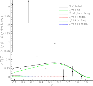
Figure 8: The $J/\psi$ energy distribution in $Z\rightarrow J/\psi+X$ with $m_{c}=1.4$ GeV, and $\mu=\mu_{BLM}$ for $J/\psi+c\bar{c}$ and $\mu=2m_{c}$ for other processes.

Combining all the above results together and timing a factor of 1.29 to include the contribution from the $\psi^{\prime}$ feed-down, we obtain the branching ratio of $J/\psi$ production in Z decay as following:

$$Br_{NLO}^{J/\psi+c\bar{c}+X}=(6.20\sim 8.38)\times 10^{-5},$$ (10)

$$Br^{frag.pro.}=(1.13\sim 1.57)\times 10^{-5},$$ (11)

$$Br^{total}=(7.33\sim 9.95)\times 10^{-5}.$$ (12)

Here we give the range of the branching ratio with the charm mass changing from 1.4 to 1.6 GeV. The total theoretical result is almost the half of the central value of the experimental measurement in Eq.(1). It is shown in Fig. 8 that the photon and gluon fragmentation processes contribute more in the lower energy region and the energy distribution can not fit the experimental data.

Furthermore, we defined a ratio as

$$R_{c\bar{c}}=\frac{\Gamma(Z\to J/\psi+c\bar{c}+X)}{\Gamma(Z\to J/\psi+X)}.$$ (13)

Using the theoretical results obtained in the CSM, the ratio is about $R^{CSM}_{c\bar{c}}=0.84~{}(0.85)$ with $m_{c}=1.4~{}(1.6)$ GeV. If we assume that the deriviation of the theoretical prediction from the central value of the experimental results is from gluon fragmentation processes in the COM that was investigated in reference Cheung:1995ka ; Baek:1996kq , the ratio can be modified as

$$R_{c\bar{c}}=\frac{1}{\Gamma_{EX}(Z\to J/\psi+X)}\{\Gamma_{CSM}(Z\to J/\psi+c\bar{c})$$

$$+R_{c\bar{c}}^{o}[\Gamma_{EX}(Z\to J/\psi X)-\Gamma_{CSM}(Z\to J/\psi X)]\},$$ (14)

where $R_{c\bar{c}}^{o}$ from gluon fragmentation processes in the COM is defined as

$$R_{c\bar{c}}^{o}=\frac{\Gamma^{g\to^{3}S_{1}(8)}(Z\to c\bar{c}+J/\psi+X)}{\sum\limits_{q}\Gamma^{g\to^{3}S_{1}(8)}(Z\to q\bar{q}+J/\psi+X)},$$ (15)

and the $q\bar{q}$ in the denominator are summed over u, d, c, s, b, and $R_{c\bar{c}}^{o}$=0.17 is obtained from reference Baek:1996kq . Then we obtain $R^{CSM+COM}_{c\bar{c}}=0.49~{}(0.41)$ for $m_{c}=1.4~{}(1.6)$GeV. The above analysis indicate that $R_{cc}$ can be used to clarify the COM contribution.

IV IV. Summary and conclusion

We have investigated all the processes that give main contributions to $J/\psi$ inclusive production in Z boson decay in the CSM. The results with NLO QCD correction are obtained. For the $Z\to J/\psi+c\bar{c}$ process, the NLO results only change the leading order results lightly, and the K factor is 1.13 with $\mu$=2$m_{c}$ and insensitive to the charm quark mass. We also use two methods to estimate the dependence of the results on the choice of renormalization scale, and these two methods give almost the same partial decay width. The K factor even fall to 0.918 by using the BLM scheme. We also include the contributions of main fragmentation processes. The total branching ratio for $Z\to J/\psi+X$ in CSM is $(7.3\sim 10.0)\times 10^{-5}$, about half of the central value of the experimental data 2.1$\times 10^{-4}$. We define $R_{c\bar{c}}=\frac{\Gamma(Z\to J/\psi c\bar{c}X)}{\Gamma(Z\to J/\psi X)}$ and obtain $R_{cc}=0.84$ for only CSM contribution and $R_{cc}=0.49$ for COM and CSM contribution together. Then $R_{cc}$ measurement could be used to clarify the COM contributions. In addition the $J/\psi$ energy distribution is inconsistent with the experimental data too. But there are large uncertainties in the experiment results on the inclusive production of $J/\psi$ in Z decay, not only the total branching ratio but also the $J/\psi$ energy distribution. Further experimental measurement with more sample data is needed to clarify the situation. Maybe in the future Z factory these processes could obtain a detailed investigation. In the calculation, the K factor for vector and axial-vector parts of $Z\to J/\psi+c\bar{c}+X$ are almost same. It may indicate that the mechanism of heavy quark fragmentation into quarkonium is dominant in this process even at NLO.

V Acknowledgments

We would like to thank Bin Gong and Hong-Fei Zhang for helpful discussion. This work is supported by the National Natural Science Foundation of China (No.10475083, 10979056 and 10935012) and by the Chinese Academy of Science under Project No. INFO-115-B01, and by the China Postdoctoral Science foundation (20090460525).

References

- (1) G. T. Bodwin, E. Braaten and G. P. Lepage, Phys. Rev. D 51, 1125 (1995) [Erratum-ibid. D 55, 5853 (1997)] [arXiv:hep-ph/9407339].
- (2) M. B. Einhorn and S. D. Ellis, Phys. Rev. D 12, 2007 (1975); S. D. Ellis, M. B. Einhorn and C. Quigg, Phys. Rev. Lett. 36, 1263 (1976); C. H. Chang, Nucl. Phys. B 172, 425 (1980); E. L. Berger and D. L. Jones, Phys. Rev. D 23, 1521 (1981); R. Baier and R. Ruckl, Nucl. Phys. B 201, 1 (1982).
- (3) N. Brambilla et al. [Quarkonium Working Group], arXiv:hep-ph/0412158; M. Kramer, Prog. Part. Nucl. Phys. 47, 141 (2001); J. P. Lansberg, Int. J. Mod. Phys. A 21, 3857 (2006).
- (4) K. Abe et al. [BELLE Collaboration], Phys. Rev. Lett. 88, 052001 (2002); K. Abe et al. [Belle Collaboration], Phys. Rev. Lett. 89, 142001 (2002); K. Abe et al. [Belle Collaboration], Phys. Rev. D 70, 071102 (2004); P. Pakhlov et al. [Belle Collaboration], Phys. Rev. D 79, 071101 (2009).
- (5) B. Aubert et al. [BABAR Collaboration], Phys. Rev. D 72, 031101 (2005).
- (6) Y. J. Zhang, Y. j. Gao and K. T. Chao, Phys. Rev. Lett. 96, 092001 (2006); Y. J. Zhang and K. T. Chao, Phys. Rev. Lett. 98, 092003 (2007); Y. J. Zhang, Y. Q. Ma and K. T. Chao, Phys. Rev. D 78, 054006 (2008); Y. Q. Ma, Y. J. Zhang and K. T. Chao, Phys. Rev. Lett. 102, 162002 (2009); B. Gong and J. X. Wang, Phys. Rev. D 77, 054028 (2008); B. Gong and J. X. Wang, Phys. Rev. Lett. 100, 181803 (2008); B. Gong and J. X. Wang, Phys. Rev. Lett. 102, 162003 (2009); W. L. Sang and Y. Q. Chen, arXiv:0910.4071 [hep-ph]; D. Li, Z. G. He and K. T. Chao, Phys. Rev. D 80, 114014 (2009); Y. J. Zhang, Y. Q. Ma, K. Wang and K. T. Chao, Phys. Rev. D 81, 034015 (2010).
- (7) B. Gong and J. X. Wang, Phys. Rev. D 80, 054015 (2009).
- (8) G. T. Bodwin, D. Kang, T. Kim, J. Lee and C. Yu, AIP Conf. Proc. 892, 315 (2007); Z. G. He, Y. Fan and K. T. Chao, Phys. Rev. D 75, 074011 (2007); G. T. Bodwin, J. Lee and C. Yu, Phys. Rev. D 77, 094018 (2008); Z. G. He, Y. Fan and K. T. Chao, Phys. Rev. D 81, 054036 (2010); Y. Jia, arXiv:0912.5498 [hep-ph].
- (9) J. M. Campbell, F. Maltoni and F. Tramontano, Phys. Rev. Lett. 98, 252002 (2007).
- (10) B. Gong and J. X. Wang, Phys. Rev. Lett. 100, 232001 (2008); B. Gong and J. X. Wang, Phys. Rev. D 78, 074011 (2008).
- (11) B. Gong, X. Q. Li and J. X. Wang, Phys. Lett. B 673, 197 (2009).
- (12) P. Artoisenet, J. M. Campbell, J. P. Lansberg, F. Maltoni and F. Tramontano, Phys. Rev. Lett. 101, 152001 (2008).
- (13) S. J. Brodsky and J. P. Lansberg, Phys. Rev. D 81, 051502 (2010); J. P. Lansberg, arXiv:1003.4319 [hep-ph].
- (14) Y. Q. Ma, K. Wang and K. T. Chao, arXiv:1002.3987 [hep-ph].
- (15) M. 1. Kramer, Nucl. Phys. B 459, 3 (1996).
- (16) P. Artoisenet, J. M. Campbell, F. Maltoni and F. Tramontano, Phys. Rev. Lett. 102, 142001 (2009); C. H. Chang, R. Li and J. X. Wang, Phys. Rev. D 80, 034020 (2009).
- (17) M. Butenschoen and B. A. Kniehl, Phys. Rev. Lett. 104, 072001 (2010).
- (18) R. Li and J. X. Wang, Phys. Lett. B 672, 51 (2009); J. P. Lansberg, Phys. Lett. B 679, 340 (2009).
- (19) Z. G. He, R. Li and J. X. Wang, arXiv:0904.1477 [hep-ph]; Z. G. He, R. Li and J. X. Wang, Phys. Rev. D 79, 094003 (2009).
- (20) Z. G. He and J. X. Wang, Phys. Rev. D 81, 054030 (2010).
- (21) B. Guberina, J. H. Kuhn, R. D. Peccei and R. Ruckl, Nucl. Phys. B 174, 317 (1980); W. Y. Keung, Phys. Rev. D 23, 2072 (1981); K. J. Abraham, Z. Phys. C 44, 467 (1989); V. D. Barger, K. m. Cheung and W. Y. Keung, Phys. Rev. D 41, 1541 (1990); K. Hagiwara, A. D. Martin and W. J. Stirling, Phys. Lett. B 267, 527 (1991) [Erratum-ibid. B 316, 631 (1993)]; E. Braaten, K. m. Cheung and T. C. Yuan, Phys. Rev. D 48, 4230 (1993); J. Jalilian-Marian, arXiv:hep-ph/9401229; P. Ernstrom, L. Lonnblad and M. Vanttinen, Z. Phys. C 76, 515 (1997); G. A. Schuler, Int. J. Mod. Phys. A 12, 3951 (1997).
- (22) K. m. Cheung, W. Y. Keung and T. C. Yuan, Phys. Rev. Lett. 76, 877 (1996); P. L. Cho, Phys. Lett. B 368, 171 (1996);
- (23) S. Baek, P. Ko, J. Lee and H. S. Song, Phys. Lett. B 389, 609 (1996);
- (24) S. Fleming, Phys. Rev. D 48, 1914 (1993).
- (25) M. Acciarri et al. [L3 Collaboration], Phys. Lett. B 453, 94 (1999).
- (26) E. M. Gregores, F. Halzen and O. J. P. Eboli, Phys. Lett. B 395, 113 (1997).
- (27) C. G. Boyd, A. K. Leibovich and I. Z. Rothstein, Phys. Rev. D 59, 054016 (1999).
- (28) J. G. Korner, D. Kreimer and K. Schilcher, Z. Phys. C 54, 503 (1992).
- (29) C. N. Yang, Phys. Rev. 77, 242 (1950).
- (30) B. Gong and J. X. Wang, Phys. Rev. D 77, 054028 (2008).
- (31) J. X. Wang, Nucl. Instrum. Meth. A 534, 241 (2004).
- (32) C. Amsler et al. [Particle Data Group], Phys. Lett. B 667, 1 (2008).
- (33) S. J. Brodsky, G. P. Lepage and P. B. Mackenzie, Phys. Rev. D 28, 228 (1983).
- (34) K. Y. Liu, Z. G. He and K. T. Chao, Phys. Rev. D 68, 031501 (2003).