Exact and approximate symmetries for light
propagation equations with higher order nonlinearity
Martin E. Garcia¹, Vladimir F. Kovalev², Larisa L. Tatarinova^1,3
1)Theoretical Physics, University of Kassel, Heinrich-Plett-Str. 40, 34132 Kassel, Germany
2) Institute for mathematical modelling RAS, Miusskaya Pl., 4-A, 125047 Moscow, Russia
3) Theoretical Physics, University of Fribourg, Chemin du Museé 3, 1700 Fribourg, Switzerland.

Abstract
For the first time exact analytical solutions to the eikonal equations in (1+1) dimensions with a refractive index being a saturated function of intensity are constructed. It is demonstrated that the solutions exhibit collapse; an explicit analytical expression for the self-focusing position, where the intensity tends to infinity, is found. Based on an approximated Lie symmetry group, solutions to the eikonal equations with arbitrary nonlinear refractive index are constructed. Comparison between exact and approximate solutions is presented. Approximate solutions to the nonlinear Schrödinger equation in (1+2) dimensions with arbitrary refractive index and initial intensity distribution are obtained. A particular case of refractive index consisting of Kerr refraction and multiphoton ionization is considered. It is demonstrated that the beam collapse can take place not only at the beam axis but also in an off-axis ring region around it. An analytical condition distinguishing these two cases is obtained and explicit formula for the self-focusing position is presented.
Keywords: Self-focusing, nonlinear Schrödinger equation, eikonal equation, symmetry group, Lie-Bäcklund symmetry.

1 Introduction

The Lie symmetry analysis of differential equations finds a great number of applications in mathematical modeling of physical problems nowadays (see, e.g. Refs. [1, 2, 3]). ). Nonlinear optics certainly occupies a particular place among these.

In 1960-ies it became evident that for an adequate mathematical description of the process of highly intense light propagation the refractive index has to depend on the intensity of applied electric field $n=n(I)$. For moderate intensities achievable at that time it was sufficient to use the so-called Kerr form of the refractive index $n=n_{0}+n_{2}I$ with $n_{0}$ being of the order of unity and $n_{2}$ varying from $10^{-19}$ to $10^{-16}$ in $({\rm W/cm^{2}})^{-1}$ depending on the material. The basic mathematical model for the propagation of intense monochromatic light that is successfully applied for a long time (see, e.g. classical monographs [4, Chapt.17] and [5], or [6, 7, 8, 9] for recent achievements) is the nonlinear Schrödinger equation (NLSE) or its approximation in the limit of geometrical optics, the eikonal equation.

For the first time, exact analytical solutions to the eikonal equations with Kerr-type refractive index in (1+1) and (1+2) dimensions were constructed by Akhmanov et al. in Ref. [10, 5]. The authors demonstrated that in both cases the solutions exhibit singularities at certain points and found explicit analytical expressions for them. Later in Ref. [11, 12] it was demonstrated that these solutions can be derived in a regular manner using the Lie-Bäcklund symmetry group admitted by the eikonal equation with Kerr refractive index.

Lie symmetry group analysis of NLSE has been performed by many authors (see, e.g. [1, Chap.16]). In particular, L. Gagnon and P. Winternitz in Ref. [13, 14, 15] found exact solutions in (1+2) dimensions, however, these solution did not correspond to localized (symmetric) intensity distributions typical for usual experimental conditions. A set of two coupled NLSE was analyzed by means of Lie group technique and the general Lie group of point symmetries, its Lie algebra, and a group of adjoint representations that corresponds to the Lie algebra were identified in Ref [16].

For the initial conditions actual for typical experiments, analytical solutions to the eikonal equation in (1+1) dimensions based on the symmetry group approach were obtained in Ref. [12]. In this paper approximate solutions for various initial intensity distributions and Kerr-type media were constructed. Later, using the similar group analysis technique approximate solutions in (1+2) dimensions for arbitrary initial intensity profile and the same form of the refractive index were found in Refs. [17, 18]. Based of the obtained solutions, the authors proceeded to investigate a global behavior of the solutions and to get explicit analytical expressions for the nonlinear self-focusing position and the value of critical power required for beam collapse.

On the other hand, modern experimental facilities allow one to achieve very intense laser beams leading to highly nonlinear media response. In such situations the Kerr approximation to the refractive index ceases to be sufficient and higher order terms with respect to power of the light intensity must be taken into account.

In the present paper we study the problem of light propagation in media with highly nonlinear response. Based on Lie symmetry group analysis, we constructed an exact solution to the eikonal equation in (1+1) dimensions for a special higher-order form of the refractive index, and also approximate analytical solutions to the problem in both (1+1) and (1+2) dimensions with the refractive index being an arbitrary function of the intensity.

The paper is organized as follows. First, after describing the model equations, we consider the problem of light propagation in (1+1) dimensions under an approximation of geometrical optics. Based of the formalism of Ref. [11] we construct the Lie-Bäcklund symmetry group admitted by the eikonal equation and consider such a superposition of the symmetry operators that yields a localized initial light intensity distribution. The use of this combination of operators gives us an exact solution of the eikonal equation with the refractive index being a saturated function of the intensity of the applied electric field. The solution exhibits a singularity: the on-axial intensity asymptotically tends to infinity at a certain propagation distance.

In the next section we construct an approximate analytical solution to the eikonal equation in (1+1) dimensions with arbitrary nonlinear media response. This solution is obtained on the basis of the approximate Lie-Bäcklund symmetry group. In order to test the applicability of used approximation the solutions obtained on the basis of exact and approximate Lie symmetry groups under the same initial conditions are compared.

The last section is devoted to the construction of approximate analytical solutions of the Schrödinger equation in (1+2) dimensions when both the refractive index and the initial intensity distributions are arbitrary. The final result is a system of algebraic equations which has to be resolved for every particular initial condition and nonlinear media response. The most typical situation in modern experiments (see e.g. [8, 9]) is the propagation of the Gaussian beam in an ionizing media, with the refractive index being a polynomial function of the light intensity. Therefore, we consider this problem as a particular application of the obtained results. Influence of the higher order nonlinear term in the refractive index on the beam collapse is considered and result is compared with the previous one obtained in Refs. [17, 18].

2 Model equations

Let us start from the NLSE:

$$i{\cal E}_{z}+{1\over 2k_{0}}\nabla_{\bot}^{2}{\cal E}+k_{0}n(|{\cal E}|^{2}){\cal E}=0\,.$$ (2.1)

Here ${\cal E}$ is the slowly-varying envelope of the electric field, $z$ is the propagation length, $k_{0}$ is the wave number $k_{0}=n_{0}\omega_{0}/c$, $\omega_{0}$ is the carrier frequency of the laser irradiation, $c$ is the velocity of light and $n=n(|{\cal E}|^{2})$ is a nonlinear refractive index in a general form (see e.g. [6, 8, 9]). Due to high intensities of light available in modern experiments the refractive index becomes highly nonlinear $n=n(|{\cal E}|^{2})$. The Laplace operator $\nabla_{\bot}^{2}$ is usually responsible for light diffraction. Explicitly, $\nabla_{\bot}^{2}=\partial_{xx}$ or $\partial_{xx}+\partial_{yy}$ for (1+1) or (1+2) dimensional cases correspondingly.

Let us now represent electric field ${\cal E}$ in the eikonal form: ${\cal E}=\sqrt{I}\exp(ik_{0}Q)$. Then, starting from Eq. (2.1), after some algebraic manipulations we obtain

$$Q_{z}=-{1\over 2}(Q_{x})^{2}+n(I)+\frac{1}{2k_{0}^{2}}\left({x^{1-\nu}\over\sqrt{I}}\partial_{x}(x^{\nu-1}\partial_{x}\sqrt{I})\right),$$ (2.2)

$$I_{z}=-\partial_{x}(IQ_{x})-(\nu-1){IQ_{x}\over{x}},$$ (2.3)

where $\nu=1$ and $\nu=2$ correspond to the (1+1) and (1+2) dimensional cases, and $x$ denotes the transverse spatial variable.

Let us differentiate the first equation with respect to $x$ and introduce a new variable $v\equiv Q_{x}$. For the sake of convenience, we introduce dimensionless variables $\tilde{I}\equiv I/I_{0}$, $\tilde{x}\equiv x/w_{\rm in}$, $\tilde{z}\equiv z/w_{\rm in}$, where $I_{0}$ is an initial peak intensity of the light beam and $w_{\rm in}$ is an initial beam radius. In what follows the dimensionless parameters shall always be used, omitting the tilde for simplicity. Moreover, let us introduce new dimensionless variables $\alpha=n_{2}I_{0}$, $\theta=(2k_{0}^{2}w_{\rm in}^{2})^{-1}$ in diffractive case. Thus, finally we get the following equations:

$$v_{z}+vv_{x}-\alpha\varphi I_{x}-\theta\partial_{x}\left({{x}^{1-\nu}\over\sqrt{I}}\partial_{x}\left(x^{\nu-1}\partial_{x}\sqrt{I}\right)\right)=0,$$ (2.4)

$$I_{z}+vI_{x}+Iv_{x}+(\nu-1){vI\over x}=0,\quad\varphi=\partial_{I}n\,.$$ (2.5)

Evidently, Eqs. (2.4), (2.5) must be supplemented with a boundary conditions. In case of collimated beam these read

$$v(0,x)=0,\hskip 56.9055ptI(0,x)=I_{0}(x),$$ (2.6)

In several cases the term with higher order derivatives can also be neglected Refs. [19] and equations (2.4), (2.5) acquire a rather simple form:

$$v_{z}+vv_{x}-\alpha\varphi I_{x}=0\,,\quad I_{z}+vI_{x}+Iv_{x}+(\nu-1){Iv\over x}=0.$$ (2.7)

Further simplification of these equations can be performed in (1+1) dimensions if one notices that in this case the system (2.7) is linear with respect to the first order derivatives. Therefore, it is convenient to use the hodograph transformation in order to transform it into a linear system of partial differential equations. In doing so, in (1+1) dimensions one obtains

$$\alpha\tau_{v}-{I\over\varphi(I)}\chi_{I}=0,\qquad\chi_{v}+\tau_{I}=0\,.$$ (2.8)

In (1+$\nu$) dimensions the Eqs. (2.7) read

$$\alpha\tau_{v}-{I\over\varphi(I)}\chi_{I}=0\,,$$ (2.9)

$$\chi_{v}+\tau_{I}+\frac{(\nu-1)v}{\chi I+\tau v}\left[\chi_{v}\left(I\tau_{I}-\tau\right)+\tau\tau_{I}-\frac{\tau^{2}}{I}-\chi_{I}^{2}\frac{I^{2}}{\varphi(I)}\right]=0\,.$$

The boundary conditions are transformed as follows: for $v=0$

$$\tau=0\,,\qquad\chi=H(I)\,,$$ (2.10)

where $H(I)$ is a function inverse to a smooth initial intensity distribution $I_{0}=I_{0}(x)$. Evidently, for example, in case of a Gaussian beam we have $\chi=\sqrt{\ln(1/I)}$.

3 An exact solution to the eikonal equations in (1+1) dimensions

Let us now construct a new exact analytical solution to Eqs. (2.8). In the present paper, for the first time, we consider a special form of the nonlinear media response with the refractive index being a saturated function of intensity. Let us rewrite Eqs. (2.8) as follows:

$$\tau_{v}-\psi(I)\chi_{I}=0,\hskip 28.45274pt\chi_{v}+\tau_{I}=0,$$ (3.11)

where $\psi=I/(\alpha\varphi)$. As a boundary condition, we take a collimated continuous wave beam with a localized symmetric intensity distribution at the entry plane of a nonlinear media

$$\tau(I,0)=0,\hskip 28.45274pt\chi(I,0)=\chi_{0}(I).$$ (3.12)

Our goal is now to construct an exact analytical solution to the system of equations (3.11) with a nonlinear function $\psi(I)$ that corresponds to a saturating dependence of the refractive index on the intensity. For this goal, $\psi$ is taken in the form ${\rm e}^{bI/I_{0}}/n_{2}I_{0}$. The refractive index corresponding to this choice of $\psi$ is presented in Fig. 1.

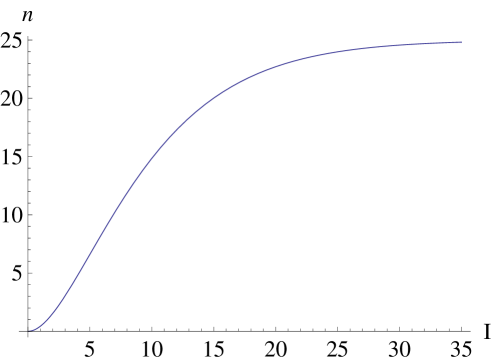
Figure 1: Nonlinear refractive index corresponding to $\psi={\rm e}^{bI}/\alpha$ as a function of the normalized intensity $I$.

Let us first sketch the broad outlines of our solution: first, we construct a Lie symmetry group admitted by Eqs. (3.11). Second, following a formal scheme reported in Refs. [20], the obtained group shall be restricted to the surface of boundary conditions: $v=0$, $\tau=0$. All derivatives of $\tau$ with respect to $I$ have to vanish too. Third, based on the requirement of vanishing of canonical coordinates of the group generators on the boundary, we shall construct such a linear superposition of them, which provides a localized beam intensity distribution. Finally, the integration of the constructed superposition shall yield a desired solution to Eqs. (3.11).

3.1 Recursion operators and Lie-Bäcklund symmetries of the second order

We start from the search for the Lie-Bäcklund symmetry group admissible by Eqs. (3.11). It is generated by the canonical infinitesimal operators [1]

$$X=f^{s}\partial_{\tau}+g^{s}\partial_{\chi}\,,$$ (3.13)

with coordinates $f^{s}$ and $g^{s}$. For the Lie-Bäcklund symmetry of arbitrary order $s>1$ the coordinates $f^{s}$ and $g^{s}$ depend on $v$, $I$, $\tau$, $\chi$ and corresponding derivatives of $\tau$ and $\chi$ up to the $s$-th order with respect to $I$

$$f^{s}=f^{s}(v,I,\tau,\chi,...,\tau_{I}^{s},\chi_{I}^{s}),\quad g^{s}=g^{s}(v,I,\tau,\chi,...,\tau_{I}^{s},\chi_{I}^{s})\,.$$

Here, the index $s$ stands for the order of the derivatives: $\tau_{I}^{s}\equiv\partial^{s}\tau/\partial I^{s}$, etc. The coordinates $f^{s}$ and $g^{s}$ are found from the determining equations that in the case of Eqs. (3.11) read [11]:

$$D_{v}(f^{s})-\psi D_{I}(g^{s})=0,\qquad D_{v}(g^{s})+D_{I}(f^{s})=0\,,$$ (3.14)

where $D_{I}$ and $D_{v}$ are operators of the total differentiation with respect to $I$ and $v$:

$$D_{I}=\partial_{I}+\sum_{s=0}^{\infty}\left(\tau_{I}^{s+1}\partial_{\tau_{I}^{s}}+\chi_{I}^{s+1}\partial_{\chi_{I}^{s}}\right),$$ (3.15)

$$D_{v}=\partial_{v}+\sum_{s=0}^{\infty}\left[\left(\psi\chi_{I}\right)_{I^{s}}\partial_{\tau_{I}^{s}}-\tau_{I}^{s+1}\partial_{\chi_{I}^{s}}\right]\,.$$

In order to solve the Eqs. (3.14), it appears more convenient to use a recursion operator [11]. The latter is defined as $2\times 2$ matrix operator transforming any linear solution of the determining equation (3.14) of the order $s$ to the solution of these equations of higher order $(s+1)$

$$L\left(\begin{array}[]{c}f^{s}\\ g^{s}\end{array}\right)=\left(\begin{array}[]{c}f^{s+1}\\ g^{s+1}\end{array}\right),\hskip 28.45274ptL=\left(\begin{array}[]{cc}L^{11}&L^{12}\\ L^{21}&L^{22}\end{array}\right),$$ (3.22)

Substitution of Eq. (3.22) into the determining equation (3.14) yields the following system of equations for the elements of $L$

$$(D_{v}L^{11}-\psi D_{I}L^{21})f^{s}+(D_{v}L^{12}-\psi D_{I}L^{22})g^{s}=0\,,$$ (3.23)

$$(D_{I}L^{11}+D_{v}L^{21})f^{s}+(D_{I}L^{12}+D_{v}L^{22})g^{s}=0,$$

which should be valid for any solutions $f^{s}$ and $g^{s}$.

Explicit formulae for the components $L^{ij}$ $(i,j=1...3)$ of recursion operators (3.22) are given in Ref. [11]

$$L_{1} = \left(\begin{array}[]{cc}0&-\psi D_{I}/\alpha\\ D_{I}&0\end{array}\right),\quad L_{2}\,\,=\,\,\left(\begin{array}[]{cc}2\sigma D_{I}-1&-\psi(1-2\sigma_{I})vD_{I}\\ (1-2\sigma_{I})vD_{I}&2\sigma D_{I}\end{array}\right),$$ (3.31)

$$\qquad\qquad L_{3}\,\,=\,\,\left(\begin{array}[]{cc}2\sigma vD_{I}-(1-\sigma_{I})v&-\psi qD_{I}-\sigma\\ qD_{I}+\psi_{I}^{-1}&2\sigma vD_{I}+v\sigma_{I}\end{array}\right),$$

where $\sigma\equiv\psi/\psi_{I}$ and $q\equiv(1-2\sigma_{I})v^{2}/2+2\int\psi_{I}^{-1}dI$. The formula for the recursion operator $L_{1}$ is valid for arbitrary nonlinearity function $\psi(I)$, while operators $L_{2}$ and $L_{3}$ arise for those functions $\psi(I)$ that fulfill the condition Ref. [11]:

$$\left({\psi\over\psi_{I}}\right)_{II}=0.$$ (3.32)

It has been just this requirement which has defined our particular choice of the function $\psi(I)$ in initial statement of the problem. For this form of $\psi$ we have:

$$\varphi=I{\rm e}^{-bI},\hskip 28.45274pt\sigma=b^{-1},\hskip 28.45274ptq=v^{2}/2-2\alpha{\rm e}^{-bI}/b^{2}.$$

In this particular case, the recursion operators read:

$$L_{1} = \left(\begin{array}[]{cc}0&-{\rm e}^{bI}D_{I}/\alpha\\ D_{I}&0\end{array}\right),\quad L_{2}\,=\,\left(\begin{array}[]{cc}2D_{I}/b-1&-{\rm e}^{bI}vD_{I}/\alpha\\ vD_{I}&2D_{I}/b\end{array}\right),$$ (3.37)

$$L_{3} = \left(\begin{array}[]{cc}2vD_{I}/b-v&\\ \left(v^{2}/2-2\alpha{\rm e}^{-bI}/b^{2}\right)D_{I}+{\rm e}^{-bI}\alpha/b&\end{array}\right.$$ (3.43)

$$\left.\begin{array}[]{cc}&\hskip 85.35826pt-{\rm e}^{bI}\left(v^{2}/2-2\alpha{\rm e}^{-bI}/b^{2}\right)D_{I}/\alpha-1/b\\ &2vD_{I}/b\end{array}\right).$$

Let us now proceed with constructing the Lie-point symmetry group admitted by Eqs. (3.11) on the basis of these operators.

An evident solution of the determining equation (3.14) is

$$f_{0}^{0}=\tau,\qquad g_{0}^{0}=\chi\,.$$ (3.44)

The action of three recursion operators $L_{i},\hskip 5.69046pti=1,2,3$ on the vector with coordinates given by Eq. (3.44) in accordance with Eq. (3.22) generates the symmetry group given by

$$f_{1}^{1}=-{\rm e}^{bI}\chi_{I}/\alpha\,,\quad f_{2}^{1}=\frac{2\tau_{I}}{b}-\tau-\frac{{\rm e}^{bI}v\chi_{I}}{\alpha}\,,$$ (3.45)

$$f_{3}^{1}=\frac{2v\tau_{I}}{b}-v\tau-\frac{{\rm e}^{bI}}{\alpha}\left(\frac{v^{2}}{2}-\frac{2\alpha{\rm e}^{-bI}}{b^{2}}\right)\chi_{I}-\frac{\chi}{b},$$

$$g_{1}^{1}=\tau_{I}\,,\quad g_{2}^{1}=v\tau_{I}+2\chi_{I}/b\,,$$

$$g_{3}^{1}=\left(\frac{v^{2}}{2}-\frac{2\alpha{\rm e}^{-bI}}{b^{2}}\right)\tau_{I}+\frac{\alpha{\rm e}^{-bI}\tau}{b}+\frac{2v\chi_{I}}{b}\,.$$

Admissible for arbitrary nonlinearity $\psi(I)$, the symmetries $f_{0}^{0}$, $g_{0}^{0}$ describe the dilatation of $\tau$ and $\chi$, whilst $f_{1}^{1}$ and $g_{1}^{1}$ generate translations along $v$-axis.

As it was formulated in Refs. [11, 20], an invariant solution to the boundary value problem, in particular the one given by Eqs. (3.11), must be found from the constructed Lie-Bäcklund symmetries under the invariance conditions

$$f=0,\qquad g=0\,,$$ (3.46)

supplemented by the original Eqs (3.11). In Eqs. (3.46) the functions $f$ and $g$ are arbitrary linear combinations of coordinates $f_{i}^{s}$ and $g_{i}^{s}$ of the group generators Eqs. (3.45) and must be chosen to satisfy the boundary conditions what in the actual case provides a localized intensity distribution.

Unfortunately, the Lie point group generators (3.45) with $s=0$ and $s=1$ are not sufficient in order to determine a linear superposition able to satisfy a smooth localized (symmetric in $\chi$) intensity distribution at the boundary. Therefore, we shall continue using the discussed approach with operators $L_{i}$ given by Eqs. (3.22) and the vectors with coordinates of Eq. (3.45) in order to find the Lie-Bäcklund symmetries of the higher order with $s>1$. However, since the further calculations are quite cumbersome, it is convenient first to find the symmetry coordinates at the boundary where they have the simplest form. Afterwards, we completely reconstruct only those that will be included into the chosen linear superposition.

Thus, at the boundary $\tau=0$, $v=0$ the recursion operators read

$$L_{1}=\left(\begin{array}[]{cc}0&-{\rm e}^{bI}D_{I}/\alpha\\ D_{I}&0\end{array}\right),\hskip 28.45274ptL_{2}=\left(\begin{array}[]{cc}2D_{I}/b-1&0\\ 0&2D_{I}/b\end{array}\right),$$ (3.51)

$$L_{3}=\left(\begin{array}[]{cc}0&2/b^{2}D_{I}-1/b\\ -2\alpha{\rm e}^{-bI}/b^{2}D_{I}+{\rm e}^{-bI}\alpha/b&0\end{array}\right),$$ (3.54)

Action of these operators on Eqs. (3.44) gives 9 symmetry operators $X_{i}$ whose coordinates $f_{i}^{s}$, $g_{i}^{s}$ are listed in the Table 1.

Table 1: Coordinates of the symmetry operators at the boundary.

	$f_{i}$	$g_{i}$
$i=0$	$0$	$\chi$
$i=1$	$-{\rm e}^{bI}\chi_{I}/\alpha$	$0$
$i=2$	$0$	$2\chi_{I}/b$
$i=3$	$2\chi_{I}/b^{2}-\chi/b$	$0$
$i=4$	$-2{\rm e}^{bI}\chi_{II}/\alpha b$	$0$
$i=5$	$0$	$-b{\rm e}^{bI}\chi_{I}/\alpha-{\rm e}^{bI}\chi_{II}/\alpha$
$i=6$	$0$	$2\chi_{II}/b^{2}-\chi_{I}/b$
$i=7$	$0$	$4\chi_{II}/b^{2}$
$i=8$	$-2{\rm e}^{bI}\chi_{II}/\alpha b-{\rm e}^{bI}\chi_{I}/\alpha$	$0$
$i=9$	$4\chi_{II}/b^{3}-4\chi_{I}/b^{2}+\chi/b$	$0$
$i=10$	$4\chi_{II}/b^{3}-2\chi_{I}/b^{2}$	$0$
$i=11$	$0$	$2\chi_{II}/b^{2}+\chi_{I}/b$
$i=12$	$0$	$-4\alpha{\rm e}^{-bI}\chi_{II}/b^{4}+4\alpha{\rm e}^{-bI}\chi_{I}/b^{3}-\alpha\chi{\rm e}^{-bI}/b^{2}$

Based on the operators presented in the Table 1, one can construct a linear superposition providing a localized intensity distribution. For instance, the equation

$$(2-{\rm e}^{bI-1})\chi_{II}+b(1-{\rm e}^{bI-1})\chi_{I}=0$$ (3.55)

has a particular solution $\chi=\sqrt{2{\rm e}^{-bI+1}-1}$. Resolving $I$ as a function of $\chi$, we get a convex symmetric on $x$ intensity distribution

$$I_{0}(\chi)=\frac{1}{b}\left(1-\ln\left(\frac{\chi^{2}+1}{2}\right)\right)\,,$$ (3.56)

which is represented by a red curve in Fig. 2.

From the Table 1 one can see that Eq. (3.55) corresponds to the following superposition of symmetry operators of the first and the second order

$$\frac{\alpha}{{\rm e}}g_{5}^{2}+\frac{b^{2}}{2}g_{7}^{2}+\frac{b^{2}}{2}g_{2}^{1}=0,$$ (3.57)

which, evidently, shall be supplemented by the equation:

$${\alpha\over{\rm e}}f_{5}^{2}+{b^{2}\over 2}f_{7}^{2}+{b^{2}\over 2}f_{2}^{1}=0.$$ (3.58)

It is easy to see that in order to find an invariant solution satisfying Eqs. (3.11) and the boundary conditions of Eq. (3.56), we have to reconstruct a complete form of the symmetry coordinates $f_{5}^{2}$, $g_{5}^{2}$ and $f_{7}^{2}$, $g_{7}^{2}$. Acting by the operator $L_{1}$ on the couple $f_{1}^{1}$, $g_{1}^{1}$, we get

$$f_{5}^{2}=-{\rm e}^{bI}\tau_{II}/\alpha\,,$$ (3.59)

$$g_{5}^{2}=-b{\rm e}^{bI}(\chi_{II}+b\chi_{I})/\alpha\,.$$

The similar procedure applied to the operator $L_{2}$ and coordinates $f_{2}^{1}$, $g_{2}^{1}$ yields:

$$f_{7}^{2}=(4\alpha-{\rm e}^{bI}v^{2}b^{2})\tau_{II}/\alpha b^{2}-4\tau_{I}/b-{\rm e}^{bI}v\chi_{I}/\alpha-4{\rm e}^{bI}v\chi_{II}/\alpha b+\tau\,,$$ (3.60)

$$g_{7}^{2}=4v\tau_{II}/b-v\tau_{I}-{\rm e}^{bI}bv^{2}\chi_{I}/\alpha+(4\alpha-{\rm e}^{bI}v^{2}b^{2})\chi_{II}/\alpha b^{2}\,.$$

These equations together with Eq. (3.45) represent the list of symmetry operators required for construction of analytical solutions.

3.2 Invariant solutions

Let us now find the desired analytical solutions. Equations (3.57)-(3.58) with expressions substituted from Eq. (3.59), (3.60) represent a system of partial differential equations

$$2bv\tau_{II}+\left(2-{\rm e}^{bI-1}-{v^{2}b^{2}{\rm e}^{bI}\over 2\alpha}\right)\chi_{II}+b\left(1-{\rm e}^{bI-1}-{v^{2}b^{2}{\rm e}^{bI}\over 2\alpha}\right)\chi_{I}=0\,,$$ (3.61)

$$-{2vb{\rm e}^{bI}\over\alpha}\chi_{II}-{vb^{2}{\rm e}^{bI}\over\alpha}\chi_{I}+\left(2-{\rm e}^{bI-1}-{v^{2}b^{2}{\rm e}^{bI}\over 2\alpha}\right)\tau_{II}-b\tau_{I}=0\,.$$ (3.62)

The first integral to the equation (3.61) can be easily found:

$$2bv\tau_{I}+\left(2-{\rm e}^{bI-1}-{v^{2}b^{2}{\rm e}^{bI}\over 2\alpha}\right)\chi_{I}+b\chi=J(v).$$ (3.63)

$J(v)$ in the above formula should be found from the comparison with Eq. (3.62). Differentiating Eq. (3.63) with respect to $v$, taking Eqs. (3.11) into account and comparing obtained expression with Eq. (3.62), one can see that $J(v)$ should be a constant. In view of a symmetric initial intensity distribution with respect to $x\to-x$ reflections we are bound to choose $J=0$. Then, substituting $\tau_{I}=-\chi_{v}$ into Eq. (3.63), we arrive at the following first order partial differential equation

$$-2bv\chi_{v}+\left(2-{\rm e}^{bI-1}-{v^{2}b^{2}{\rm e}^{bI}\over 2\alpha}\right)\chi_{I}+b\chi=0,$$ (3.64)

which can be integrated with a standard technique.

Integration of Eq. (3.64) gives two first integrals,

$$J^{1}=\frac{-\chi^{2}}{v},\hskip 28.45274pt\quad J^{2}=\frac{-1}{v}\left(2{\rm e}^{1-bI}-1+\frac{b^{2}{\rm e}}{2\alpha}v^{2}\right).$$ (3.65)

Here and in what follows one has to keep in mind that a negative value of $v$ corresponds to the focusing beam for the positive values of $x$.

Now we are in a position to find a particular solution $\chi(v,I)$ for the Eqs. (3.11) satisfying the boundary conditions Eq. (3.56). Let us first notice that from the system of equations (3.11) a linear second order partial differential equation

$$\alpha\chi_{vv}+({\rm e}^{bI}\chi_{I})_{I}=0,$$ (3.66)

can be derived. Based on the result obtained in Eqs. (3.65), one can search for the solution to Eq. (3.66) based on the following Ansatz

$$\chi^{2}=-vQ^{2}(J^{2}),$$ (3.67)

Substituting Eq. (3.67) into Eq. (3.66) after some calculations we get:

$$Q_{\mu\mu}-Q/4=0,$$ (3.68)

where $\mu={\rm arcsinh}(J^{2}/\sqrt{2b^{2}{\rm e}/\alpha})$. Equation (3.68) has an evident general solution

$$Q=C_{1}{\rm e}^{-\mu/2}+C_{2}{\rm e}^{\mu/2},$$

where $C_{1}$ and $C_{2}$ are constants which should be found from the boundary conditions.

Taking the Eq. (3.67) into account we obtain the expression for $\chi$:

$$\chi=(-v)^{1/2}\left[C_{1}{\rm e}^{-\mu/2}+C_{2}{\rm e}^{\mu/2}\right]\,,$$ (3.69)

where ${\rm e}^{\mu/2}$ is to be found from the equation:

$$\quad\sinh\mu = \sqrt{\frac{\alpha}{2b^{2}{\rm e}}}\frac{-1}{v}\left(2{\rm e}^{1-bI}-1+\frac{b^{2}{\rm e}}{2\alpha}v^{2}\right)\,.$$ (3.70)

Now we can express ${\rm e}^{\mu}$ from Eq. (3.70)

$${\rm e}^{\mu}=K/2\pm\sqrt{K^{2}/4+1}\,,$$ (3.71)

where

$$K\equiv\sqrt{\frac{2\alpha}{b^{2}{\rm e}}}\frac{-1}{v}\left(2{\rm e}^{1-bI}-1+\frac{b^{2}{\rm e}}{2\alpha}v^{2}\right).$$

Summarizing, the following solutions to the system of equations (3.11) is obtained:

$$\chi={1\over\sqrt{2}}\sqrt{\left(2{\rm e}^{1-bI}-1+{b^{2}{\rm e}v^{2}\over 2\alpha}\right)+\sqrt{\left(2{\rm e}^{1-bI}-1+{b^{2}{\rm e}v^{2}\over 2\alpha}\right)^{2}+{2b^{2}{\rm e}v^{2}\over\alpha}}}.$$ (3.72)

In order to find the second function $\tau(I,v)$, we shall integrate the original equation (3.11) keeping the result (3.72) in mind. From Eqs. (3.11) we have

$$\tau=\frac{1}{\alpha}\int\limits_{0}^{v}{\rm d}v{\rm e}^{bI}\chi_{I}\,.$$ (3.73)

For the sake of convenience, let us introduce a new variable $\xi$:

$$\cosh(\xi)\equiv{2{\rm e}^{1-bI}+{b^{2}{\rm e}v^{2}\over 2\alpha}+1\over\sqrt{8{\rm e}^{1-bI}}}.$$ (3.74)

Then

$$\chi_{I}={b\over 4\sqrt{\Theta}}{{\rm e}^{1-bI\over 2}-\sqrt{2}{\rm e}^{\xi+1-bI}\over\sinh(\xi)}.$$

The expression for $\tau$ becomes:

$$\tau={1\over b}\int_{\xi_{0}}^{\xi}{(a{\rm e}^{\xi}-1)^{1/2}\over-v}d\xi=\left.\sqrt{{\rm e}\over 2\alpha}\ln\left({2{\rm e}^{\xi}\over a}-1+\sqrt{\left({2{\rm e}^{\xi}\over a}-1\right)^{2}-1}\right)\right|_{\xi_{0}}^{\xi},$$

where $a\equiv\sqrt{2}\exp((1-bI)/2))$. Taking the boundary conditions into account, the final solution reads:

$$\tau={\sqrt{{2\rm e}\over\alpha}}\ln\left({\rm e}^{(bI-1)/2}\sqrt{\frac{(\chi^{2}+1)}{2}}+\sqrt{{\rm e}^{bI-1}\frac{(\chi^{2}+1)}{2}-1}\right).$$ (3.75)

After direct substitution of Eqs. (3.72), (3.75) into Eqs. (3.11) and a tedious calculation it is possible to verify that the obtained functions $\chi(I,v)$ and $\tau(I,v)$ are indeed exact analytical solutions for the formulated boundary value problem. In Fig. 2 we plot the intensity beam distribution at different propagation distances calculated on the basis of the found solutions Eqs. (3.72), (3.75).

Figure 2: Beam profile at different propagation distances. $\alpha=3,$ $b=1$. Red curve - $z=0,$ black curve - $z=0.8$.

Let us now examine the obtained result a little more closely. Firstly let us find the total radius of the beam as a function of propagation distance $z$. For this goal, it is necessary to determine where the intensity implicitly given by Eqs. (3.72), (3.75) intersects the surface of $x=0$. Putting $I=0$ in Eq. (3.75), we find $\chi|_{I=0}=\pm\sqrt{2{\rm e}-1}$. Substituting this number into Eq. (3.72) one can deduce that $v=0$ and, consequently, $x=\pm\sqrt{2{\rm e}-1}$. Thus, the phase gradient at the beam edge is equal to zero, the total radius of the beam is a constant and does not depend on the propagation length. By the numerical integration of the solutions Eqs. (3.72), (3.75) one can verify their consistence with energy conservation, i.e. $\int I(x,z)dx$ from $x=\sqrt{2{\rm e}-1}$ to $x=-\sqrt{2{\rm e}-1}$ is a constant.

The fact that the total radius of the beam for the case under consideration remains constant and does not depend on $z$ is a new one and completely different from all exact analytical results obtained so far. It was demonstrated earlier [5, 12] that for the Kerr nonlinearity the total beam radius decreases upon beam propagation. In the present case, the beam shape and peak intensity are thus the only parameters depending on the propagation distance.

Evolution of the beam peak intensity, which for the symmetry reasons has to be situated on the beam axis, can be easily found from Eq. (3.75). Putting $x=0$, $v=0$ we have

$$\frac{z}{b}\sqrt{\frac{2\alpha}{\rm e}}=\frac{2}{bI}\ln\left((1/\sqrt{2})\,{\rm e}^{(bI-1)/2}+\sqrt{(1/2)\,{\rm e}^{bI-1}-1}\right).$$ (3.76)

On-axial intensity distribution versus the propagation distance is presented in Fig. 3 for $\alpha=0.001,$ $b=0.2.$ We see that the intensity monotonically increases and tends to infinity for $z$ approaching a critical value denoted as a self-focusing position $z_{\rm sf}$. Its exact value can be found from direct analysis of the Eq. (3.76). Considering Eq. (3.76) in the limit $I\to\infty$ one obtains

$$z_{\rm sf}=b\sqrt{{\rm e}\over 2\alpha}.$$ (3.77)

A detailed investigation of the Eqs. (3.72), (3.75) shows that the solutions exhibit no singularities before this point.

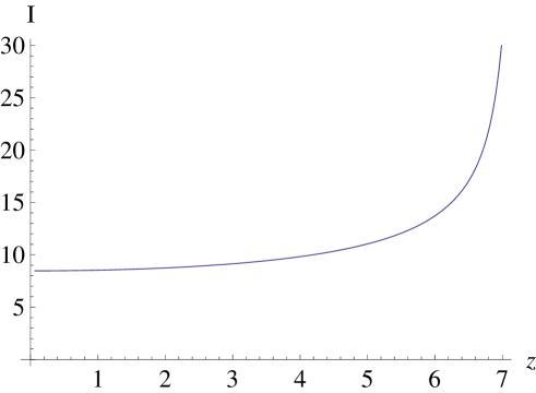
Figure 3: On-axial intensity distribution versus the propagation distance.

4 Approximate solutions to the eikonal equation in (1+1) dimensions with arbitrary refractive index

Because it is not possible to construct an exact analytical solution for every desired form of the refractive index and the boundary conditions, let us now present here a possible way to obtain approximate analytical solutions. We shall start from the Eqs. (2.8). Under certain conditions (see e.g. [19]), $\alpha$ can be considered as a small parameter. Due to its smallness, we will search for an approximate symmetries group operator:

$$X=p\partial_{\tau}+q\partial_{\chi},$$

with coordinates in form of a power series in $\alpha$:

$$p=\sum\alpha^{i}p^{i}\,,\qquad q=\sum\alpha^{i}q^{i}\,,\qquad i=0,\ldots,\infty\,.$$ (4.78)

In case of Eqs. (2.8), the determining equations read:

$$\left(D_{w}^{0}+\alpha D_{w}^{1}\right)p-\frac{I}{\varphi(I)}D_{I}q=0\,,\quad\left(D_{w}^{0}+\alpha D_{w}^{1}\right)q+\alpha D_{I}p=0\,,$$ (4.79)

where $w=v/\alpha$ and

$$D_{w}^{0}=\partial_{w}+\sum_{s=0}^{\infty}\left((I/\varphi)\chi_{I}\right)_{I^{s}}\partial_{\tau_{I}^{s}}\,,\quad D_{w}^{1}=-\sum_{s=0}^{\infty}\tau_{I}^{s+1}\partial_{\tau_{I}^{s}}\,.$$

Substituting Eqs. (4.78) into Eqs. (4.79) we arrive at a following system of recurrent differential equations:

$$D_{w}^{0}q^{i}+(1-\delta_{i,0})\left(D_{w}^{1}q^{i-1}+D_{I}(p^{i})\right)=0\,,$$ (4.80)

$$D_{w}^{0}p^{i}+(1-\delta_{i,0})D_{w}^{1}p^{i-1}-\frac{I}{\varphi}D_{I}(q^{i})=0\,.$$ (4.81)

The system (4.80)-(4.81) can be solved sequentially starting from a given $g^{0}$. Thus, integration of Eqs. (4.80)-(4.81) gives

$$p^{i}=\int dw \left\{\sum_{s=0}^{\infty}(1-\delta_{i,0})\tau_{I}^{s+1}\partial_{\chi_{I}^{s}}p^{i-1}\right.$$ (4.82)

$$\left.+\frac{I}{\varphi}\left[\partial_{I}+\sum_{s=0}^{\infty}\left(\tau_{I}^{s+1}\partial_{\tau_{I}^{s}}+\chi_{I}^{s+1}\partial_{\chi_{I}^{s}}\right)\right]q^{i}\right\}+P^{i}\,,$$

$$q^{i}=(1-\delta_{i,0})\int dw \left\{\sum_{s=0}^{\infty}\tau_{I}^{s+1}\partial_{\chi_{I}^{s}}q^{i-1}\right.$$

$$\left.-\left[\partial_{I}+\sum_{s=0}^{\infty}\left(\tau_{I}^{s+1}\partial_{\tau_{I}^{s}}+\chi_{I}^{s+1}\partial_{\chi_{I}^{s}}\right)\right]p^{i-1}\right\}+Q^{i}\,.$$

Here $P^{i}$ and $Q^{i}$ are arbitrary functions of invariants

$$I,\quad\chi_{I}^{s},\quad\mbox{and}\quad\tilde{\tau_{I}^{s}}=\tau_{I}^{s}-w\sum_{p=0}^{s}C^{s}_{p}(\partial^{p}(I/\varphi)/\partial I^{p})\chi_{I}^{s-p+1},\quad i\geq 1\,,$$

and $C^{s}_{p}$ is the binomial coefficient (see Ref. [12]).

Let us now put

$$q^{0}=0,\quad p^{0}=1+2I\chi\chi_{I}/\varphi\,.$$ (4.83)

This choice of $p^{0}$ corresponds to a special form of initial light beam

$$\int_{0}^{I_{0}}(\varphi/I)\,dI=-x^{2}\,.$$

For nonlinearities $\varphi(I)$ relevant to particular physical situations, such form of initial intensity distribution is very similar to the Gaussian profile. It should be stressed that, in general, there are no restrictions on the initial intensity distribution $I=I_{0}(x)$, the present choice is made only for the sake of further simplicity.

Substituting this function into equation for $g^{1}$ we get

$$q^{1}=wD_{I}(2I\chi\chi_{I}/\varphi)+G^{1}={\varphi(\tilde{\tau}-\tau)\over I\chi_{I}}D_{I}(2I\chi\chi_{I}/\varphi)+G^{1}=-2(\tau\chi)_{I}\,,$$ (4.84)

where the term with ${\tilde{\tau}}$ was included into a new arbitrary function $\tilde{G^{1}}$, which was later put equal to zero.

Using this result, we can calculate $p^{1}$ in a similar way. We get

$$p^{1}=-{I\over\varphi}\left(\tau^{2}{\varphi\over I}\right)_{I}\,.$$ (4.85)

Finally, up to the first order of $\alpha$, the coordinates of the approximate symmetries group generator read

$$q=-2\alpha(\tau\chi)_{I}\,,\quad p=1+2I\chi\chi_{I}/\varphi-\alpha\frac{I}{\varphi}\left(\frac{\tau^{2}\varphi}{I}\right)_{I}\,.$$ (4.86)

Taking Eqs. (2.8) into account, we rewrite the desired symmetry group operator as follows

$$R=\left(1-\alpha\tau^{2}{(\varphi/I)_{I}\over\varphi/I}\right)\partial_{\tau}-2\chi\partial_{w}+2\alpha\tau\partial_{I}\,.$$ (4.87)

Integration of the Lie equations corresponding to the point symmetry operator (4.87) gives us the three first integrals whose particular form depends on the choice of $\varphi=\varphi(I)$. We write these integrals by introducing the new function $\phi(I)$, such that $\phi_{I}=\varphi/I$:

$$J_{1}=\chi\,,\quad J_{2}=\alpha\tau^{2}\phi_{I}-\phi\,,\quad J_{3}=w+\frac{\chi}{\sqrt{\alpha}}\int\frac{{\rm d}\phi}{\sqrt{\phi_{I}}\sqrt{\phi+J_{2}}}\,.$$ (4.88)

Now, the solution is a function of these first integrals fulfilling the boundary conditions. This means that values of $J_{i}$ are taken from the boundary conditions when $\tau\to 0$ and $\chi\to x^{\prime}$. Hence we rewrite (4.88) in the following form

$$x^{\prime}=\chi\,,\qquad\phi(I_{0}(x^{\prime}))=-\alpha z^{2}I^{2}\phi_{I}+\phi\,,$$ (4.89)

$$x^{\prime}\sqrt{\alpha}\int\limits^{\phi(I_{0}(x^{\prime}))}\frac{{\rm d}\phi}{\sqrt{\phi_{I}}\sqrt{\phi+J_{2}}}=v+(x-vz)\sqrt{\alpha}\int\limits^{\phi}\frac{{\rm d}\phi}{\sqrt{\phi_{I}}\sqrt{\phi+J_{2}}}\,.$$

In the particular case of Kerr nonlinearity $\varphi=1$, we arrive at the solution previously obtained in Ref. [12].

Let us now compare the approximate solutions with the exact solution constructed in the previous section. In order to satisfy the boundary condition Eq. (3.56), $p^{0}$ is taken in the form

$$p^{0}=2b{\rm e}+2I\chi\chi_{I}/\varphi\,,$$

Then the generator (4.87) reduces to:

$$R=(2b{\rm e}+\alpha\tau^{2})\partial_{\tau}-2\chi\partial_{w}+2\alpha\tau\partial_{I}\,,$$

and yields an approximate solution:

$$\left(\left(x-vz\right)^{2}+1\right){\rm e}^{bI}=\alpha I^{2}z^{2}+2{\rm e}\,,$$ (4.90)

$$v=-\sqrt{\frac{2\alpha}{{\rm e}}}\frac{1}{b}(x-vz)\,{\rm arctg}\left(Iz\sqrt{\frac{\alpha}{2{\rm e}}}\right)\,.$$

On-axial intensity distribution is given by expression ${\rm e}^{bI}-2{\rm e}=\alpha I^{2}z^{2}$, which exhibits no singularities. The on-axial intensity monotonically increases upon propagation. However, the function $v(x,t)$ can exhibit singularities which, due to the symmetry of the problem, are expected to be on the beam axis. Let us investigate this behavior more closely. In the vicinity of the beam axis, $v_{x}$ can be approximated as

$$v_{x}=-\sqrt{\frac{2\alpha}{{\rm e}}}\frac{1}{b}\,{\rm arctg}\left(Iz\sqrt{\frac{\alpha}{2{\rm e}}}\right)\left(1-z\sqrt{\frac{2\alpha}{\rm e}}\frac{1}{b}\,{\rm arctg}\left(Iz\sqrt{\frac{\alpha}{2{\rm e}}}\right)\right)^{-1}\,.$$

Then, the position of a singularity at the beam axis (what corresponds to the rays intersection) can be found from the system of equations:

$$1-z_{sf}\sqrt{\frac{2\alpha}{\rm e}}\frac{1}{b}\,{\rm arctg}\left(Iz_{sf}\sqrt{\frac{\alpha}{2{\rm e}}}\right)=0\,,\qquad\alpha z_{sf}^{2}I^{2}=-2{\rm e}+{\rm e}^{bI}\,.$$ (4.91)

The numerical solution of Eqs. (4.91) yields $z_{\rm sf}\approx 1.03\,b\sqrt{{\rm e}/2\alpha}$. As one sees, this result is very similar to Eq. (3.77) obtained from the exact solution. The similar tendency has been observed in Ref. [21] for the Kerr refractive index: an approximate solution provides a longer self-focusing distance in comparison to exact one.

5 Approximate solution to the Schrödinger equations with arbitrary refractive index in (1+2) dimensions

In this section we shall turn to the construction of approximate solutions for the NLSE (2.1) in (1+2) dimensions in media with arbitrary nonlinearity. Such a mathematical model describes the propagation of a continuum wave beam in cylindrical geometry and has great number of application to particular physical situations (see e.g. [6, 8, 9]). Let us begin with equations (2.4), (2.5) supplemented by the boundary condition

$$v(0,x)=0\,,\qquad I(0,x)=N(x)\,,$$ (5.92)

which corresponds to a collimated beam with arbitrary initial intensity distribution.

As usual, we start from construction of the Lie-Bäcklund symmetry operator of the form

$$X=\kappa\partial_{v}+\lambda\partial_{I}\,.$$

The determining equations read:

$$D_{z}\kappa +vD_{x}\kappa+\kappa v_{1}-\alpha\varphi D_{x}\lambda-\alpha\varphi_{I}I_{1}\lambda$$ (5.93)

$$-\beta\left(B_{I}\lambda+B_{I_{1}}D_{x}\lambda+B_{I_{2}}D_{x}^{2}\lambda+B_{I_{3}}D_{x}^{3}\lambda\right)=0,$$

$$D_{z}\lambda +ID_{x}\kappa+vD_{x}\lambda+\lambda v_{1}+\kappa I_{1}+\frac{v\lambda}{x}+\frac{\kappa I}{x}=0\,,$$

where

$$B=D_{x}\left({D_{x}(xD_{x}\sqrt{I})\over x\sqrt{I}}\right),\quad v_{s}\equiv\frac{\partial^{s}v}{\partial x^{s}}\,,\quad I_{s}\equiv\frac{\partial^{s}I}{\partial x^{s}}\,,$$ (5.94)

$$D_{x}=\partial_{x}+\sum_{s=0}^{\infty}(v_{s+1}\partial_{v_{s}}+I_{s+1}\partial_{I_{s}}),$$

and $D_{z}$ we present as $D_{z}=D_{z}^{0}+D_{z}^{1},$ where

$$D_{z}^{0}=\partial_{z}-\sum_{s=0}^{\infty}\left(D_{x}^{s}(vv_{1})\partial_{v_{s}}+\left[D_{x}^{s+1}(Iv)+D_{x}^{s}\left(\frac{Iv}{x}\right)\right]\partial_{I_{s}}\right)\,,$$

$$D_{z}^{1}=\sum_{s=0}^{\infty}\left[D_{x}^{s}(\alpha\varphi I_{1}+\beta B)\right]\partial_{v_{s}}\,.$$

Since $\alpha$ and $\beta$ in Eqs. (2.7) can be considered as small parameters, we will search for $\kappa$ and $\lambda$ in form of a series expansion in powers of $\alpha$ and $\beta$

$$\kappa=\sum_{i,j=0}^{\infty}\alpha^{i}\beta^{j}\kappa^{(i,j)},\qquad\lambda=\sum_{i,j=0}^{\infty}\alpha^{i}\beta^{j}\lambda^{(i,j)}\,.$$ (5.95)

and restrict ourselves only to the first order corrections

$$\kappa=\kappa^{0}+\kappa^{1}+O(\alpha^{2},\beta^{2},\alpha\beta)\,,\qquad\lambda=\lambda^{0}+\lambda^{1}+O(\alpha^{2},\beta^{2},\alpha\beta)\,,$$ (5.96)

where $\kappa^{0}\equiv\kappa^{(0,0)}$, $\lambda^{0}\equiv\lambda^{(0,0)}$, $\kappa^{1}\equiv\alpha\kappa^{(1,0)}+\beta\kappa^{(0,1)}$, and $\lambda^{1}\equiv\alpha\lambda^{(1,0)}+\beta\lambda^{(0,1)}$. Let us now write down the determining equations keeping only the linear terms with respect to $\alpha$ and $\beta$. We get

$$M_{0}\kappa^{0} =0\,,\qquad M_{1}\lambda^{0}+M_{2}\kappa^{0}=0\,,$$ (5.97)

$$M_{0}\kappa^{1} +D_{z}^{1}\kappa^{0}-\alpha D_{x}(\varphi\lambda^{0})$$

$$-\beta\left[B_{I}\lambda^{0}+B_{I_{x}}D_{x}\lambda^{0}+B_{I_{xx}}D^{2}_{x}\lambda^{0}+B_{I_{xxx}}D^{3}_{x}\lambda^{0}\right]=0\,,$$

$$M_{1}\lambda^{1} +D_{z}^{1}\lambda^{0}+M_{2}\kappa^{1}=0\,,$$

where

$$M_{0}=D_{z}^{0}+vD_{x}+v_{1}\,,$$ (5.98)

$$M_{1}=D_{z}^{0}+vD_{x}+v_{1}+v/x\,,$$

$$M_{2}=ID_{x}+I_{1}+I/x\,.$$

Let us now following to Ref. [17] put

$$\kappa^{0}=\frac{1}{2}D_{x}(v^{2})\,,\qquad\lambda^{0}=\frac{1}{x}D_{x}(Ivx)\,.$$ (5.99)

Evidently this choice satisfies the zero-order Eqs. (5.97) and the invariance conditions: $\kappa^{0}=0$, $\lambda^{0}=0$ at the boundary. Then $\kappa^{1}$ can be found from the first of the first-order equations in Eq. (5.97) that is rewritten as

$$M_{0}\left(\kappa^{1}+\alpha\varphi I_{1}+\beta D_{x}\left(\frac{D_{x}(xD_{x}\sqrt{I})}{x\sqrt{I}}\right)\right)=0.$$ (5.100)

The solution of this equation is expressed in terms of invariants of the operator $M_{0}$,

$$\kappa^{1}=D_{x}\left(S(\chi)-\alpha\Phi-\beta\frac{D_{x}(xD_{x}\sqrt{I})}{x\sqrt{I}}\right)\,,$$ (5.101)

where

$$\varphi=\partial_{I}\Phi\,,\quad S(\chi)\equiv\alpha\Phi(N(\chi))+\beta\frac{(\chi(\sqrt{N(\chi)})_{\chi})_{\chi}}{\chi\sqrt{N(\chi)}}\,.$$ (5.102)

Inserting this result into the second of the first-order equations in Eq. (5.97) we get the equation for the function $q^{1}$

$$M_{1}\lambda^{1}+{D_{x}\over x}\left(IzD_{x}S(\chi)\right)=0\,.$$

It is easy to show by direct substitution that the formula above can be rewritten as

$$M_{0}(x\lambda^{1})+D_{x}\left(IzD_{x}S(\chi)\right)=0\,.$$

This equation can be integrated in a same as (5.100). Then one gets

$$x\lambda^{1}=-D_{x}(xIzS_{\chi}).$$

Finally, up to the first order in the small parameters, the Lie-Bäcklund symmetry operators in the canonical form read:

$$\kappa=vv_{1}+D_{x}\left(S(\chi)-\alpha\Phi-\beta\frac{D_{x}(xD_{x}\sqrt{I})}{x\sqrt{I}}\right)\,,$$ (5.103)

$$\lambda=v\left(I_{1}+\frac{I}{x}\right)+Iv_{x}-z\left[I(1-zv_{1})S_{\chi\chi}+\left(I_{1}+\frac{I}{x}\right)S_{\chi}\right]\,.$$ (5.104)

We notice that based on (2.4), (2.5) Eq. (5.103) can be rewritten as follows:

$$\kappa=v_{z}-(1-v_{x}z)S_{\chi}\,.$$

Together with Eq. (5.103), the equation above lead to two relations:

$$v=zS_{\chi}\,,$$ (5.105)

$$v_{z}=(1-v_{x}z)S_{\chi}\,,$$ (5.106)

that have to be fulfilled in order to preserve the invariance requirement $\kappa=0$, $\lambda=0$.

Now, keeping the relation between the canonical form of the symmetries operator and the point symmetries group operator [1] in mind we can write down the group symmetry operator:

$$R =\left(1+z^{2}S_{\chi\chi}\right)\partial_{z}+S_{\chi}\partial_{v}+(zS_{\chi}+vz^{2}S_{\chi\chi})\partial_{x}$$ (5.107)

$$-Iz\left(\left(1+{vz\over x}\right)S_{\chi\chi}+{1\over x}S_{\chi}\right)\partial_{I}\,.$$

Operator Eq. (5.107) is similar to the one obtained previously in Ref. [12] for a collimated beam with the exception that the $S(\chi)$ now contains an arbitrary function $\Phi$. The generator (5.107) yields a system of characteristic equations:

$${dz\over 1+z^{2}S_{\chi\chi}}={dv\over S_{\chi}}={d\chi\over-v}={d\ln(Ix)\over-zS_{\chi\chi}}.$$ (5.108)

This system of equations can be easily integrated after taking into account Eq. (5.105). The second and third equations of (5.108) give

$$S+{S_{\chi}^{2}z^{2}\over 2}=S(\mu)\,,$$ (5.109)

where $\mu$ corresponds to the value of $\chi$ at the boundary. The third and the fourth of Eqs. (5.108) yield another invariant $Ix/S_{\chi}$, what can also be rewritten as

$$I=N(\mu){\chi\over x}{S_{\chi^{2}}\over S_{\mu^{2}}}\,,$$ (5.110)

where $N(\chi)$ is an initial intensity profile.

From the first and the second of Eq. (5.108) we have $v_{z}=S_{\chi}/(1+z^{2}S_{\chi\chi})$. Taking Eq. 5.106) and $D_{x}S(\chi)=(1-zv_{x})S_{\chi}$ into account and using $2\chi S_{\chi}=S_{\chi^{2}}$, we finally arrive at a relation between $x$ and $\chi$:

$$x=\chi(1+2z^{2}S_{\chi^{2}})\,.$$ (5.111)

Summarizing, the solutions are presented by the equations:

$$v(x,z)={x-\chi\over z}\,,\qquad I(x,z)=N(\mu)\frac{\chi}{x}\frac{S_{\chi^{2}}}{S_{\mu^{2}}}\,,$$ (5.112)

where $\chi$ and $\mu$ are defined as functions of $z$ and $x$ via relations

$$x=\chi\left(1+2z^{2}S_{\chi^{2}}\right)\,,\qquad S(\mu)=S(\chi)+\frac{S_{\chi}^{2}z^{2}}{2}\,,$$ (5.113)

These solutions describe the evolution of a collimated continuous wave laser beam with arbitrary initial intensity distribution in media with arbitrary nonlinear response. In case of Kerr refractive index, these solutions were investigated in details in Refs. [17, 18]. obtained solutions to more complicated forms of the refractive index.

We shall consider refractive index of the form

$$n=n_{0}+n_{2}I-\sigma_{K}I^{K}.$$ (5.114)

Here, the second term in the right hand side represents the usual Kerr response, and the last term is responsible to the multiphoton ionization of the media in case of sufficiently strong electric field; the $K$ then corresponds to the number of photons required for a simultaneous ionization, and $\sigma_{K}$ to the ionization rate. If at the entry plane of the nonlinear media the Gaussian intensity distribution is fulfilled, one obtains

$$S=\alpha\exp(-\chi^{2})-\alpha\gamma\exp(-K\chi^{2})/K+\beta(\chi^{2}-2),$$ (5.115)

where $\gamma=K\sigma_{K}I_{0}^{K-1}/n_{2}.$

Let us write the first of Eq. (5.112) as follows

$$v={2zS_{\chi^{2}}\over 1+2z^{2}S_{\chi^{2}}}\,,$$ (5.116)

where $S_{\chi^{2}}=-\alpha{\rm e}^{-\chi^{2}}+\alpha\gamma{\rm e}^{-K\chi^{2}}+\beta$. Here $v$ is a single-valued function of $x$ if the function $x=\chi(x)$ can be determined from the first of equations (5.113) uniquely. In order to find the region of multivaluedness let us investigate the function $Y\equiv\chi(1+2z^{2}S_{\chi^{2}})$. We find where its first and second derivatives with respect to $\chi$ vanish.

From equation $Y_{\chi}=0$ we have

$$1+2z^{2}S_{\eta}(\eta)+4z^{2}\eta S_{\eta\eta}(\eta)=0\,,$$ (5.117)

where $\eta\equiv\chi^{2}.$ Equation $Y_{\chi\chi}=0$ gives

$$\chi\left(3S_{\eta\eta}(\eta)+2\eta S_{\eta\eta\eta}(\eta)\right)=0\,.$$ (5.118)

Evidently, this equation is fulfilled if $\chi=0$, or the expression in the brackets is equal to zero. In the first case, we observe the singularity at the beam axis, in the second case, the singularity takes place at the point $\eta=\eta_{cr}$ which should be found numerically from equation $3S_{\eta\eta}(\eta)+2\eta S_{\eta\eta\eta}(\eta)=0$ for each particular form of $S(\eta).$

In the first case, when $\chi=0$, expression (5.116) becomes singular on the beam axis at the point

$$z_{\rm sf}=1/\sqrt{2(\alpha(1-\gamma)-\beta)}.$$ (5.119)

The beam collapse at the beam axis occurs if $\alpha>\alpha\gamma+\beta$. This result is very similar to the case of Kerr nonlinearity considered in Refs. [17, 18], the difference only coming from the presence of the $\gamma$ term under the square root. If $\alpha<\alpha\gamma+\beta$, the beam collapse does not take place on the beam axis.

In the second case, if $\chi\neq 0$, position of the singularity can be found form the magnitude of $\eta_{cr}$ which gives us $\chi=\pm\sqrt{\eta_{cr}}$ and $S_{\eta}(\eta)|_{\eta=\eta_{cr}}$. Starting form Eq. (5.117), we can find the coordinates of the singularity position:

$$z=\left.\sqrt{-1\over 2(S_{\eta}+2S_{\eta\eta})}\right|_{\eta=\eta_{cr}},\hskip 28.45274ptx=\left.\pm 2\sqrt{\eta}\left({S_{\eta\eta}\over S_{\eta}+2S_{\eta\eta}}\right)\right|_{\eta=\eta_{cr}}.$$ (5.120)

Let us now consider two particular choices of the parameters in the refractive index. Let $\alpha=0.01,$ $\beta=0.001,$ $\gamma=0.1$, $K=6$. At the beam axis $x=0$, the formula (5.119) gives us the self-focusing position $z_{\rm sf}\approx 7.9$. Eq. (5.118) has one solution $\eta\simeq 1.5$, but the corresponding magnitude of the self-focusing distance defined by Eqs. (5.120) is imaginary. This means that one observes only one self-focusing position at the beam axis. The beam intensity, $I(x)$, and the phase gradient, $v(x)$, as a function of $x$ at different propagation distances are presented on Fig. 4.

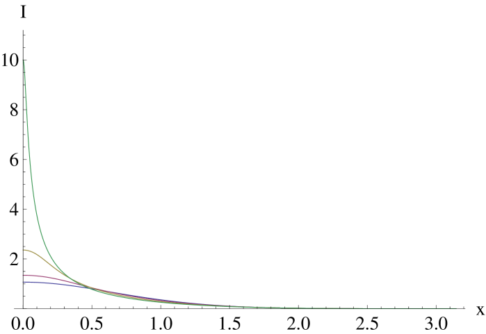
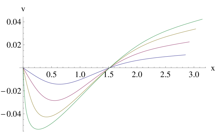
Figure 4: The beam intensity (left panel) and the phase gradient (right panel) distributions upon the transverse coordinate $x$ for $\alpha=0.01,$ $\beta=0.001,$ $\gamma=0.1$ and $K=6$. The transition near the beam axis $x\to 0$ from the bottom to the top on the left panel and from the top to the bottom on the right panel correspond to curves at different distances $z=2,$ $z=4,$ $z=6,$ $z=7.5$.

Let us now assume that $\alpha=0.01,$ $\beta=0.001,$ $\gamma=0.6$, $K=8$, then Eq. (5.118) gives us two solutions $\eta_{1}=1.5$ and $\eta_{2}\simeq 0.11$. Similar to the previous case, the first value of $\eta=\eta_{1}$ gives no singularity. However, substituting $\eta_{2}$ into Eqs. (5.120), we get position where the beam collapse take place $x\simeq 0.1,\,z\simeq 8.$ Considering behavior of the solutions at the beam axis, we see that the intensity increases, and the solution becomes singular at the point $z_{cr}\simeq 13$, that already behind the distance at which the first singularity appeared. The intensity and phase gradient at different propagation distances are presented on the Fig. 5.

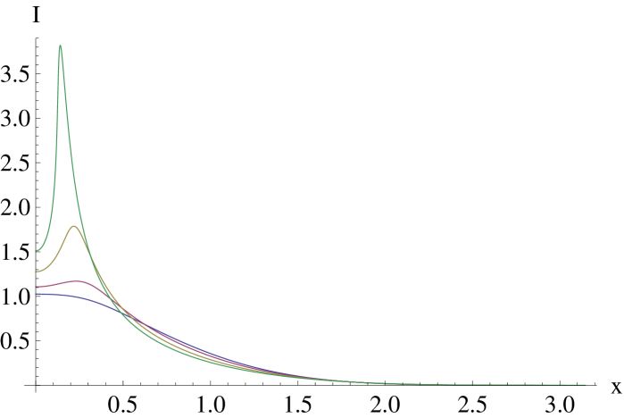
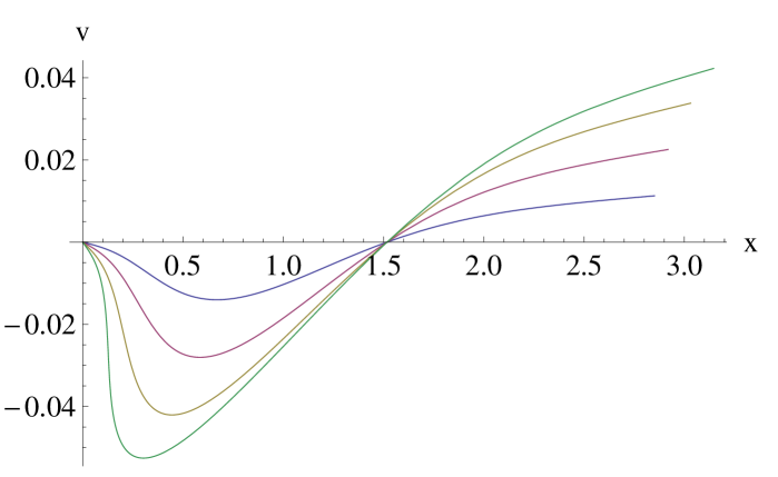
Figure 5: The beam intensity (left panel) and the phase gradient (right panel) distributions upon the transverse coordinate $x$ for $\alpha=0.01,$ $\beta=0.001,$ $\gamma=0.6$ and $K=8$. The transition near the beam axis $x\to 0$ from the bottom to the top on the left panel and from the top to the bottom on the right panel correspond to curves at different distances $z=2,$ $z=4,$ $z=6,$ $z=7.5$.

Summarizing this part of the work, we can notice that for the form of the refractive index Eq. (5.114) considered as an example in the present paper, several pictures in the global behavior of the solutions can be distinguished: i) if the solution of Eq. (5.118) provide us with only imaginary values of $z_{\rm sf}$, there is no beam collapse at all, ii) the singularity appears at the beam axis, ii) the singularity appears around the beam axis at the circle with radius given by Eqs. (5.120).

6 Conclusion

In the presented paper, making use of the Lie symmetry analysis, we constructed exact and approximate analytical solutions for the problem of light propagation in highly nonlinear media. For the first time exact analytical solutions (3.72), (3.75) to the eikonal equations in (1+1) dimensions were found with nonlinear refractive index being a saturated function of intensity. It was shown that at a certain point at the beam axis Eq. (3.77) the solution becomes singular: intensity tends to infinity asymptotically when the light propagation distance approaches $z_{\rm sf}=b\sqrt{{\rm e}/2\alpha}$.

In case of the eikonal equations with arbitrary nonlinear refractive index we constructed approximate analytical solutions. For the case of initial intensity distribution given by equation (3.56), the approximate solution was compared with the exact one (3.72), (3.75). It was shown that a value of the self-focusing position provided by an approximate solution was very close to the magnitude obtained from the exact formula (3.77).

In the last section we considered a nonlinear Schrödinger equation in (1+2) dimensions with arbitrary refractive index. An approximate symmetry group admitted by both this equation and boundary conditions corresponding to collimated beam with arbitrary initial intensity distribution was constructed. The solution was presented in the form of algebraic equations (5.112) which must be analyzed for each particular form of the refractive index and the initial intensity distribution. As an example, the case of two-term nonlinear refractive index Eq. (5.114) was examined in details. We obtained an explicit formula for the self-focusing position Eq. (5.119) and demonstrated that, for this form of the refractive index, the beam collapse can also take place outside the beam axis.

Bibliography

- [1] CRC Hanbook of Lie Group Analysis of Differential Equations, ed. N.H. Ibragimov, (CRC Press Inc., Boca Raton, 1994–1996).
- [2] V. F. Kovalev and D. V. Shirkov, Renorm-group symmetry for functionals of boundary value problem solutions, J. Phys. A: Math. Gen. 39, 8061-8073 (2006).
- [3] V. F. Kovalev and D. V. Shirkov, Renormgroup symmetries for solutions of nonlinear boundary value problems, Physics Uspekhi, 51, 815 (2008).
- [4] Y.R. Shen, The principles of nonlinear optics, John Wiley & Sons, Inc., New York - Chicester -Brisbane Toronto - Singapore, 1984.
- [5] S. A. Akhmanov, A. P. Sukhorikov, R. V. Khokhlov, Self-focusing and diffraction of light in a nonlinear medium, Sov. Phys. Usp. 10, 609-636 (1968).
- [6] R. W. Boyd, Nonlinear Optics, (Academic Press, Amsterdam, Tokyo, 2003).
- [7] J.-C. Diels, W. Rudolph, Ultrashort Laser Pulse Phenomena, (Elsevier, Amsterdam, 2006).
- [8] A. Couairon, A. Mysyrowicz, Femtosecond filamentation in transparent media, Phys. Rep. 441, 47-189 (2007).
- [9] L. Bergé, S. Skupin, R. Nuter, J. Kasparian, J.-P. Wolf, Ultrashort filaments of light in weakly-ionized, optically-transparent media, Rep. Prog. Phys. 70, 1633-1684 (2007).
- [10] S. A. Akhmanov, R. V. Khokhlov, A. P. Sukhorukov, On the self-focusing and self-chanelling of intense laser beams in nonlinear medium, Sov. Phys. JETP 23, 1025-1033 (1966).
- [11] V. F. Kovalev, and V. V. Pustovalov, Group and renormgroup symmetry of a simple model for nonlinear phenomena in optics, gas dynamics and plasma theory, Mathem. Comp. Modelling 25, 165-179 (1997).
- [12] V. F. Kovalev, Renormgroup symmetries in problems of nonlinear geometrical optics, Theor. Math. Phys. 111, 686-702 (1997).
- [13] L. Gagnon and P. Winternitz, Exact solutions of the cubic and quintic nonlinear Schr dinger equation for a cylindrical geometry, Phys. Rev. A 39, 296 306 (1998).
- [14] L. Gagnon and P. Winternitz, Lie symmetries of a generalised nonlinear Schrodinger equation: I. The symmetry group and its subgroups, J. Phys. A: Math. Gen. 21, 1493-1511 (1988).
- [15] L. Gagnon and P. Winternitz, Lie symmetries of a generalised non-linear Schrodinger equation. II. Exact solutions. J. Phys. A: Math. Gen. 22, 469-497 (1989).
- [16] V. I. Pulov, I. M. Uzunov and E. J. Chacarov, Solutions and laws of conservation for coupled nonlinear Schr dinger equations: Lie group analysis, Phys. Rev. E 57, 3468 3477 (1998).
- [17] V. F. Kovalev, Renonrmalization group analysis for singularities in the wave beam self-focusing problem, Theor. Math. Phys. 113, 719-730 (1990).
- [18] V. F. Kovalev, V. Yu. Bychenkov, V. T. Tikhonchuk, Renormalization-group approach to the problem of light-beam self-focusing, Phys. Rev. A 61, 033809(1-10) (2000).
- [19] L. L. Tatarinova, M. E. Garcia, Exact solutions of the eikonal equations describing self-focusing in highly nonlinear geometrical optics, Phys. Rev. A 78, 021806(R)(1-4) (2008).
- [20] D. V. Shirkov, V. F. Kovalev, The Bogoliubov renormalization group and solution symmetry in mathematical physics, Phys. Rep. 352, 219-249 (2001).
- [21] V. F. Kovalev, Approximate transformation groups and renormgroup symmetries, Nonlinear Dynamics, 22, 73-83 (2000).