Spectral and polarization dependencies of luminescence by hot carriers in graphene

Abstract

The luminescence caused by the interband transitions of hot carriers in graphene is considered theoretically. The dependencies of emission in mid- and near-IR spectral regions versus energy and concentration of hot carriers are analyzed; they are determined both by an applied electric field and a gate voltage. The polarization dependency is determined by the angle between the propagation direction and the normal to the graphene sheet. The characteristics of radiation from large-scale-area samples of epitaxial graphene and from microstructures of exfoliated graphene are considered. The averaged over angles efficiency of emission is also presented.

I Introduction

Electro- and photoluminescence of the bulk semiconductor materials and structures have been used for more than fifty years both in the characterization these materials and in the operation of light-emitting devices. 1 Emission of radiation in the far- and mid-IR spectral regions caused by nonequilibrium charge carriers also have been studied for two-dimensional systems, see reviews in Ref. 2 , and for the transitions between the subbands of heavy and light holes in $p$-Ge. 3 In graphene processes of emission of radiation are actual due to the effective heating of carriers by dc electric field 4 ; 5 ; 6 and due to the the efficient interband transitions excited by photons. 7 In this work we analyze spectral and polarization dependences of emission for interband transitions (on frequencies exceeding the frequency of relaxation) induced by hot carriers in a bipolar graphene. The characteristics of radiation are considered for two cases of emission: (a) from large-scale-area samples of epitaxial graphene and (b) from microstructures of exfoliated graphene, see Figs. 1a and 1b, respectively. The analysis is based on the quasiclassical kinetic equation for 3D photons where the interaction with 2D carriers is described by the boundary condition at graphene sheet (see Ch. 4 in 8 and a similar approach for the case of acoustic phonon emission 9 ).

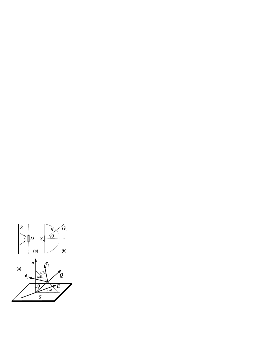
Figure 1: Geometry of luminescence by hot carriers from graphene sheet of: (a) a large-scale-area sample ($S$), with detector ($D$) placed in the near-zone; (b) a finite-size sample ($S_{1}$), where $G_{r}$ is the energy flow in the far-zone. (c) Polarization characteristics of radiation. Here n is the normal to 2D plane, $\textbf{e}_{1,2}$ are the unit vectors of polarization, and Q is the wave vector. Angles $\theta$ and $\phi$ define propagation direction and in-plane orientation, respectively.

Spectral dependencies of emission are determined by the character of distributions of nonequilibrium electrons and holes, wherein a heating electric field modifies not only an effective temperature of carriers but also electron and hole concentrations. These nonequilibrium characteristics are dependent on a lattice temperature, $T$, a strength of applied electric field, E, and a gate voltage $V_{g}$. Due to direct interband transitions and a linear character of the energy spectrum of graphene, a radiation with frequency $\omega$ is emitted for transitions between electron ($e$) and hole ($h$) states with the momentum $p_{\omega}=\hbar\omega/2v_{W}$, where $v_{W}\approx 10^{8}$cm/s is the characteristic velocity of the Weyl-Wallace model (degenerated both on spin and valley quantum numbers). 10 It appears that spectral dependence of radiation is proportional to the product of $e$- and $h$-distribution functions, $f_{ep_{\omega}}f_{hp_{\omega}}$, and the maximum energy of emitted photons is determined by both the effective temperature of carriers, $T_{c}$, and the electron and hole concentrations. The spectral behavior of radiation is strongly dependent on the densities of carriers, which in turn are essentially dependent on $V_{g}$.

The polarization dependence of emission results from the chiral character of the neutrino-like states, 11 so that the matrix elements of interband transition are dependent on orientation of 2D momentum, p. 5 Due to this, a strong dependence of polarization from the angle $\theta$, between the direction of propagation of radiation and the normal vector to the graphene sheet (see Fig. 1), is obtained. In addition, a weak the current-induced anisotropy of distributions, $\propto(eE\tau_{m}/\bar{p})^{2}\ll 1$ (here $\tau_{m}$ is the momentum relaxation time and $\bar{p}$ is the characteristic momentum of carriers), leads only to a weak anisotropy of emission. Such weak variations of polarization are determined by the angle, $\phi$, with respect to the direction of the in-plane applied field, and pertinent contributions are omitted below.

The paper is organized as follows. The basic equations governing the emission of radiation in graphene are considered in Sec. II. In Sec. III, we analyze the polarization characteristics and the spectral dependencies of radiation. The concluding remarks and discussion of the assumptions used are given in the last section.

II Basic equations

Emission of radiation due to the interband transitions of nonequilibrium carriers in graphene is described by the Wigner distribution function of photons, $N_{\bf Qr}^{\mu\mu^{\prime}}$ with the polarization indexes $\mu=1,2$. Outside of the graphene sheet, $N_{\bf Qr}^{\mu\mu^{\prime}}$ obeys the following kinetic equation 8

$${\bf v}_{\bf Q}\cdot\nabla_{\bf r}N_{\bf Qr}^{\mu\mu^{\prime}}=J_{R}.$$ (1)

Here ${\bf v}_{\bf Q}=\partial\omega_{Q}/\partial{\bf Q}=\widetilde{c}{\bf Q}/Q$ is the velocity of photon with the frequency $\omega_{Q}$, $\textbf{Q}\equiv(\textbf{q},q_{\bot})$ is the wave vector of photon with the in-plane (transverse) component, q ($q_{\bot}$), and $\widetilde{c}$ is the speed of light in the medium around the graphene sheet with dielectric permittivity $\epsilon$. The collision integral $J_{R}$ describes the relaxation of photon distribution outside of graphene (the glancing photons, with $q_{\bot}\to 0$, are not considered). The boundary condition, around the graphene sheet placed at $z=0$, takes form

$$\upsilon_{\bot}N_{\bf Qr}^{\mu\mu^{\prime}}\left|{}_{z=-0}^{z=+0}=I_{\bf Q}^{\mu\mu^{\prime}}\right.,$$ (2)

where $\upsilon_{\bot}=\widetilde{c}q_{\bot}/Q$ and $I_{\bf Q}^{\mu\mu^{\prime}}$ determines the speed of spontaneous emission due to interband transitions. Within the collisionless approximation, $I_{\bf Q}^{\mu\mu^{\prime}}$ is determined by the direct interband transitions ($l\neq l^{\prime}$) between the states $|l{\bf p}\rangle$ and $|l^{\prime}{\bf p}\rangle$, with distribution functions $f_{l{\bf p}}$ and $f_{l^{\prime}{\bf p}}$, and is given by 8

$$I_{\bf Q}^{\mu\mu^{\prime}}=4\frac{(2\pi e)^{2}}{\epsilon L^{2}\omega_{Q}}\sum\limits_{ll^{\prime}{\bf p}}\left\langle l{\bf p}\left|{\bf e}_{{\bf Q}\mu}\cdot{\bf\hat{v}}\right|l^{\prime}{\bf p}\right\rangle^{*}\left\langle l{\bf p}\left|{\bf e}_{{\bf Q}\mu^{\prime}}\cdot{\bf\hat{v}}\right|l^{\prime}{\bf p}\right\rangle$$

$$\times f_{l{\bf p}}(1-f_{l^{\prime}{\bf p}})\delta(\hbar\omega_{Q}+\varepsilon_{l^{\prime}p}-\varepsilon_{lp}).~{}~{}~{}~{}$$ (3)

Here the factor 4 comes from the spin and the valley degeneracy, $L^{2}$ is the normalization area, and the polarization vectors, ${\bf e}_{{\bf Q}\mu}$, are defined by relations $(\textbf{Q}\cdot\textbf{e}_{{\bf Q}\mu})=0$ and $(\textbf{e}_{{\bf Q}\mu}^{\ast}\cdot\textbf{e}_{{\bf Q}\mu^{\prime}})=\delta_{\mu\mu^{\prime}}$. It is convenient to choose them with the angles $\pm\pi/4$ towards the plane formed by the vectors Q and n, see Fig. 1. Point out that in Eq. (3), due to the energy conservation, contribute only the direct interband transitions between the states with $l=1$ and $l^{\prime}=-1$, where the $\delta$-function obtains the form $\delta(\hbar\omega_{Q}-2v_{W}p)$.

Thus, the characteristics of emission (its intensity, spectral dependency, and polarization) are expressed via $N_{\bf Qr}^{\mu\mu^{\prime}}$ determined by Eqs. (1)-(3). The energy flow density is defined by the standard formula 8 ; 12

$${\bf G}_{\bf r}=\sum\limits_{\mu}\int\frac{d{\bf Q}}{(2\pi)^{3}}{\bf v}_{\bf Q}\hbar\omega_{Q}N_{\bf Qr}^{\mu\mu}.$$ (4)

The polarization properties are characterized by the Stokes parameters, $\xi_{x}$, $\xi_{y}$, and $\xi_{z}$ which are introduced by relations 12

$$\xi_{x}=\frac{N_{\bf Q}^{12}+N_{\bf Q}^{12\ast}}{N_{\bf Q}},\;\;\;\xi_{y}=i\frac{N_{\bf Q}^{12}-N_{\bf Q}^{12\ast}}{N_{\bf Q}},$$

$$\xi_{z}=\frac{N_{\bf Q}^{11}-N_{\bf Q}^{22}}{N_{\bf Q}},~{}~{}~{}~{}~{}~{}~{}~{}~{}~{}~{}~{}~{}~{}~{}~{}$$ (5)

where $N_{\bf Q}=\sum_{\mu}N_{\bf Q}^{\mu\mu}$ determines an intensity of radiation propagated along $\bf Q$. Below we restrict ourselves by the nonabsorbing medium, $J_{R}\to 0$, and consider (a) the in-plane homogeneous geometry, which is corresponded to a large-area sample of epitaxial graphene, and (b) a small-size sample of exfoliated graphene.

For the case (a), Eqs. (1) and (2) have the solution

$$N_{{\bf Q}z}^{\mu\mu^{\prime}}=\frac{I_{\bf Q}^{\mu\mu^{\prime}}}{\upsilon_{\bot}}\left\{\begin{array}[]{*{20}c}{\theta(z),}&{q_{\bot}>0}\\ {\theta(-z),}&{q_{\bot}<0}\\ \end{array}\right.$$ (6)

which describes emitted radiation with $q_{\bot}>0$ ($q_{\bot}<0$) at $z>0$ ($z<0$). The only nonvanishing component of the energy flow density $G_{\bot}$ is directed along $0Z$ and it is given by

$$G_{\bot}=\sum\limits_{\mu}\int\frac{d{\bf Q}}{(2\pi)^{3}}\hbar\omega_{Q}I_{\bf Q}^{\mu\mu}=\int\limits_{0}^{\infty}d\omega\int\limits_{(q_{\bot}>0)}d\Omega_{\bf Q}\frac{\partial^{2}G}{\partial\omega\partial\Omega},$$ (7)

where the differential flow, $\partial^{2}G/\partial\omega\partial\Omega$, is introduced

$$\frac{\partial^{2}G}{\partial\omega\partial\Omega}=\frac{\hbar\omega^{3}}{(2\pi\tilde{c})^{3}}\sum\limits_{\mu}I_{\bf Q}^{\mu\mu}.$$ (8)

In addition, it is convenient to introduce the frequency-dependent differential flow $dG/d\omega=\int\limits_{(q_{\bot}>0)}d\Omega_{\bf Q}(\partial^{2}G/\partial\omega\partial\Omega)$ that is averaged over the solid angle $\Omega_{\bf Q}$ subtended by the infinite plane.

Considering emission from the sample placed within the in-plane region $S_{1}$ [case (b)], we suppose that $N_{\bf Qr}^{\mu\mu^{\prime}}$ is zero outside of $S_{1}$-region (i.e., we neglect by the edge diffraction effects). Thus, one obtains the solution

$$N_{\bf Qr}^{\mu\mu^{\prime}}={\cal N}_{\bf Q}^{\mu\mu^{\prime}}\left(x-\frac{q_{x}}{q_{\bot}}z,y-\frac{q_{y}}{q_{\bot}}z\right),$$ (9)

$${\cal N}_{\bf Q}^{\mu\mu^{\prime}}(x,y)\equiv\frac{I_{\bf Q}^{\mu\mu^{\prime}}}{\upsilon_{\bot}},~{}~{}~{}~{}(x,y)\in S_{1}$$

with ${\cal N}_{\bf Q}^{\mu\mu^{\prime}}(x,y)=0$ outside of the $S_{1}$-region. In the far zone, $R\gg\sqrt{S_{1}}$ (see Fig. 1b), the tangential components of $\bf G$ vanish and the radial component of energy flow takes form:

$$G_{r}(\theta)=\frac{S_{1}}{R^{2}}\int_{0}^{\infty}d\omega\frac{\partial^{2}G}{\partial\omega\partial\Omega},$$ (10)

where the differential flow, introduced by Eq. (8), appears.

It is convenient to rewrite the speed of spontaneous emission Eq. (3) by making the replacement from the band quantum numbers $(l,l^{\prime})$ to the electron-hole representation, when the distributions $f_{l{\bf p}}$ are substituted for electron and hole distributions as: $f_{1{\bf p}}\to f_{e{\bf p}}$ and $(1-f_{-1{\bf p}})\to f_{h-{\bf p}}$. Then Eq. (3) obtains the form

$$I_{\bf Q}^{\mu\mu^{\prime}}=4\frac{(2\pi ev_{W})^{2}}{\epsilon L^{2}\omega_{Q}}\sum\limits_{\bf p}M_{\mu\mu^{\prime}}(\varphi)~{}~{}~{}~{}~{}$$

$$\times f_{e{\bf p}}f_{h,-{\bf p}}\delta(\hbar\omega_{Q}-2v_{W}p),~{}~{}~{}~{}~{}~{}$$

$$M_{\mu\mu^{\prime}}(\varphi)={\left\langle{1{\bf p}\left|{{\bf e}_{{\bf Q}\mu}\cdot{\bf\hat{v}}}\right|-1{\bf p}}\right\rangle^{*}\left\langle{1{\bf p}\left|{{\bf e}_{{\bf Q}\mu^{\prime}}\cdot{\bf\hat{v}}}\right|-1{\bf p}}\right\rangle},$$ (11)

where the interband matrix elements $M_{\mu\mu^{\prime}}(\varphi)$ are dependent only on the orientation of the unit vectors of polarization and on the angle $\varphi$, giving the orientation of the momentum, ${\bf p}=(p\cos\varphi,p\sin\varphi)$.13 Neglecting a weak anisotropy of distributions $f_{e,h{\bf p}}$, one can use in Eq. (11) the averaged over the $\bf p$-plane angle (such an average, over the angle $\varphi$, is denoted using the overline) matrix element

$$\overline{M}_{\mu\mu^{\prime}}=\frac{e_{\mu}^{x}e_{\mu^{\prime}}^{x}+e_{\mu}^{y}e_{\mu^{\prime}}^{y}}{2}=\frac{1}{2}\left(\delta_{\mu\mu^{\prime}}-\frac{\sin^{2}\theta}{2}\right),$$ (12)

where $\theta=\widehat{{\bf n},{\bf Q}}$, see Fig. 1. As a result, the speed of spontaneous emission, Eq. (11), we can rewrite as $I_{\omega\theta}^{\mu\mu^{\prime}}\equiv I_{\bf Q}^{\mu\mu^{\prime}}$, due to its dependence only on $\omega$ and $\theta$. Finally, completing in Eq. (11) the integral over $p$ by using the energy $\delta$-function, we obtain the speed of emission as

$$I_{\omega\theta}^{\mu\mu^{\prime}}=\frac{(2\pi ev_{W})^{2}}{2\epsilon\omega}\overline{M}_{\mu\mu^{\prime}}f_{ep_{\omega}}f_{hp_{\omega}}\rho_{\hbar\omega/2},$$ (13)

where $\rho_{E}=2E/\pi(\hbar v_{W})^{2}$ is the density of states and the distributions are taken at the characteristic momentum $p_{\omega}$. Therefore, the spectral and polarization dependencies of radiation are presented in Eq. (13) by the separate factors.

III Emission characheristics

Here we study the polarization or the spectral characteristics of the luminescence determined by Eqs. (5) or (4), (7), and (II), respectively. Distributions of nonequilibrium electrons and holes are described by the quasiequilibrium Fermi functions $f_{kp}\approx\left\{\exp\left[\left(v_{W}p-\mu_{k}\right)/T_{c}\right]+1\right\}^{-1}$ with effective temperature $T_{c}$ and the chemical potentials $\mu_{k}$, that determine the concentrations of electrons and holes, $n_{e}$ and $n_{h}$. 5 Instead of the concentrations $n_{e,h}$ it is convenient to introduce the surface charge $e\Delta n=e(n_{e}-n_{h})$, that is defined by the gate voltage $V_{g}$, and the total concentration $n=n_{e}+n_{h}$, that is defined by a character of the generation-recombination processes. In addition, the effective temperature $T_{c}$ of the hot electrons and holes can be estimated from experimental data 14 and from calculations.5 ; 6

III.1 Polarization of radiation

First, let us consider the polarization characteristics of radiation emitted. Here we use that the spectral and polarization dependencies are separated, see Eqs. (6) and (13), and the Stokes parameters (5) are expressed only through $\overline{M}_{\mu\mu^{\prime}}$, Eq. (12). Therefore the polarization of radiation is independent of the frequency or the character of the carriers distributions. Then, for the geometry of Fig 1b, in the far-zone by using Eq. (13) in Eq. (5) we obtain that $\xi_{y}=\xi_{z}=0$ and

$$\xi_{x}=\frac{2\overline{M}_{12}}{\overline{M}_{11}+\overline{M}_{22}}=-\frac{\sin^{2}\theta}{1+\cos^{2}\theta},$$ (14)

which determines a degree of the linear polarization as function of $\theta$. For the geometry of Fig. 1a for any plane wave contribution, with given ${\bf Q}$, we again can introduce the Stokes parameters Eq. (5) and they have the same form as for the geometry of Fig 1b.

From Eq. (14) it follows that for the normal propagation, $\theta\to 0$, the emitted radiation becomes nonpolarized, in agreement with the absence of any preferential direction over the graphene sheet. If to take into account a weak lateral anisotropy of the carriers distributions induced by the applied electric field ${\bf E}$ then additional dependence of the polarization characteristics appears from the mutual orientation of the vectors $\bf E$ and $\bf Q$ defined by the angle $\phi$, see Fig. 1c. This small addendum also depends on $\omega$ and the form of the distribution functions of the carriers. For the glancing propagation, at $\theta\to\pi/2$, Eq. (14) shows that emitted radiation is fully linearly polarized, in a 2D plane parallel to the graphene sheet. Appearance of the universal angular dependence Eq. (14) allows for separation of the interband contributions in graphene from any possible background emission (e.g., from a substrate, a cover layer or a gate).

III.2 Spectral dependencies

Next, we study the spectral dependencies and the efficiency of radiation emitted by hot carriers for the geometries shown in Figs. 1a and 1b. Performing the summation over polarization of Eq. (13), we present the differential flows $dG/d\omega$ and $\partial^{2}G/\partial\omega\partial\Omega$, see Eq. (8), through $\sum_{\mu}I_{\omega\theta}^{\mu\mu}$. These differential flows give the relevant intensities of radiation, by Eqs. (7) and (10). The differential flow Eq. (8) obtains the form

$$\frac{\partial^{2}G}{\partial\omega\partial\Omega}=G_{c}A\left(\frac{\hbar\omega}{2T_{c}}\right)\left(1+\cos^{2}\theta\right),$$ (15)

where it is introduced the characteristic density of energy $G_{c}=\sqrt{\epsilon}e^{2}(T_{c}/\hbar c)^{3}/\pi^{2}$ and the spectral behavior is determined by the following dimensionless function

$$A\left(\frac{\hbar\omega}{2T_{c}}\right)=\left(\frac{\hbar\omega}{2T_{c}}\right)^{3}f_{ep_{\omega}}f_{hp_{\omega}}.$$ (16)

The angular dependence in Eq. (15) is given by the factor $(1+\cos^{2}\theta)$; i. e., the intensity of the glancing emission there is two times smaller than the normal one. The differential flow Eq. (15) integrated over the solid angle of half-space gives

$$\frac{dG}{d\omega}=\frac{8\pi}{3}G_{c}A\left(\frac{\hbar\omega}{2T_{c}}\right),$$ (17)

i.e., $dG/d\omega$ is expressed through the function Eq. (16). For $T_{c}=$300 K and $\epsilon\simeq$3 we estimate the characteristic density of energy, $G_{c}\propto T_{c}^{3}$, as $G_{c}\simeq 1.06\times 10^{-17}$ J/cm².

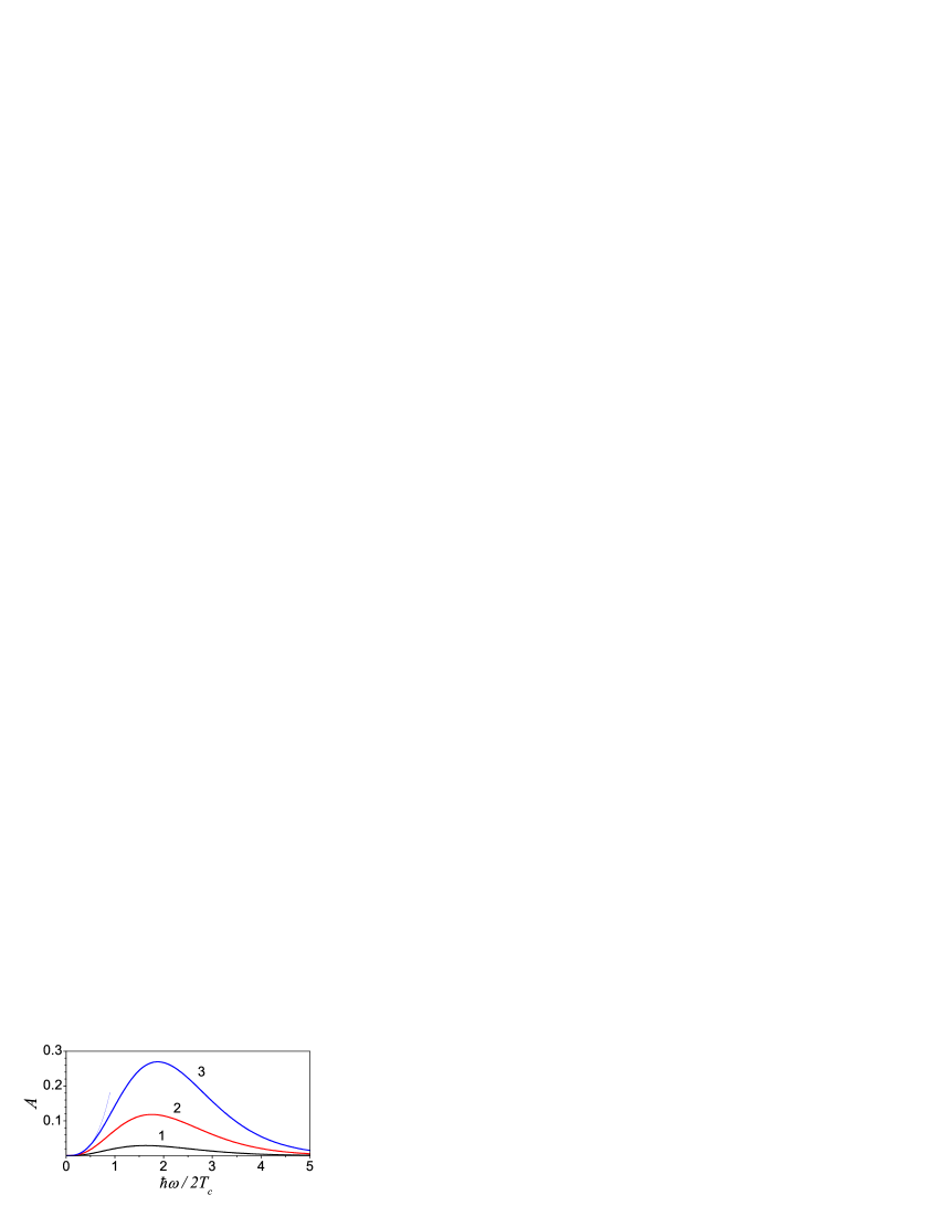
Figure 2: (Color online) Dimensionless function $A$ versus $\hbar\omega/2T_{c}$ for the intrinsic graphene case at different generation-recombination levels determined by ratio: $n/n_{T_{c}}=$0.5 (1), 1 (2) and 1.5 (3).

Thus, the spectral characteristics of radiation are expressed through the function $A(\hbar\omega/2T_{c})$ and it is shown in Fig. 2 for an intrinsic graphene. Here, one defines the degree of nonequilibrium of the electron-hole pairs concentration as the ratio, $n/n_{T_{c}}$, of the total concentration $n$ to pertinent equilibrium one (at $T_{c}$ and $\mu_{e}=\mu_{h}=0$), where $n_{T_{c}}=(\pi/3)(T_{c}/\hbar v_{W})^{2}$. This ratio also characterizes the effectiveness of generation-recombination processes. It is seen from Fig. 2 that as $n/n_{T_{c}}$ grows the intensity of emission essentially increases and the spectral maximum of radiation, localized at $\hbar\omega\sim T_{c}$, is slowly shifted. For high frequencies $A(\hbar\omega/2T_{c})$, Eq. (16), is exponentially decreasing as $\exp(-\hbar\omega/T_{c})$ and at low frequencies this function grows $\propto\omega^{3}$ (the latter asymptotic dependence is shown in Fig. 2 by the dashed curve, for $n/n_{T_{c}}=1.5$).

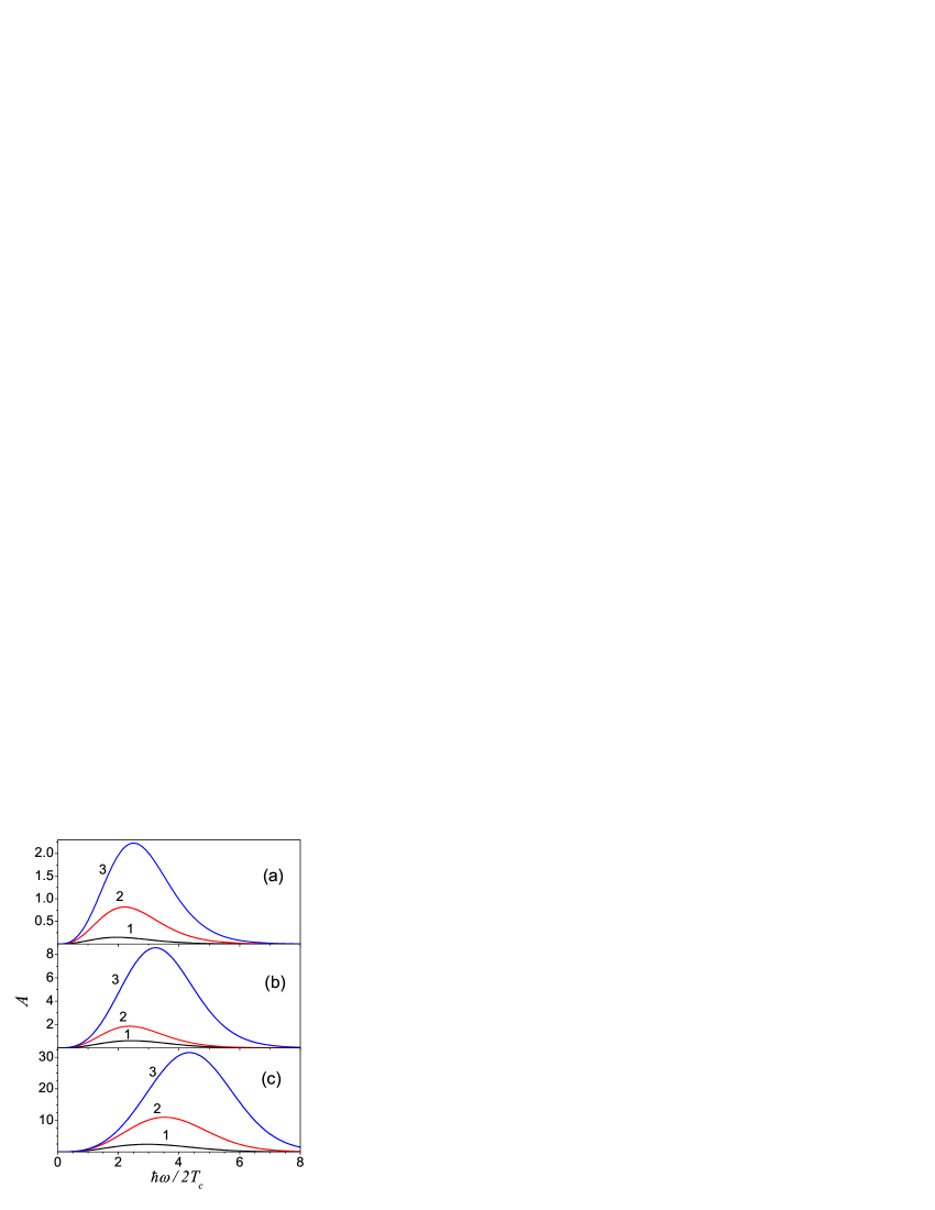
Figure 3: (Color online) Dimensionless function $A$ versus $\hbar\omega/2T_{c}$ for doped graphene at $T_{c}=$300 K and at different generation-recombination conditions determined by ratio: $n/\Delta n=$1.25 (1), 2 (2) and 3 (3). Doping levels are governed by gate voltages: $V_{g}=$5 V (a), 10 V (b), and 20 V (c).

For the doped graphene the spectral maximum is shifted to higher energies due to the Pauli blocking effect arising as the gate voltage, $V_{g}$, increases (compare Figs. 3a, 3b, and 3c plotted for $T_{c}=$300 K). Here the total concentration of carriers is defined by the ratio $n/\Delta n$, where $e\Delta n$ gives the surface charge density controlled by $V_{g}$. Present calculations are conducted for a typical graphene structure on SiO₂ substrate of the thickness 300 nm. As in intrinsic graphene, for growing concentration the intensity of emission increases, moreover, for growing $V_{g}$ the maximum also rapidly becomes larger. For high energies the spectrum of emission becomes exponentially decreasing.

,

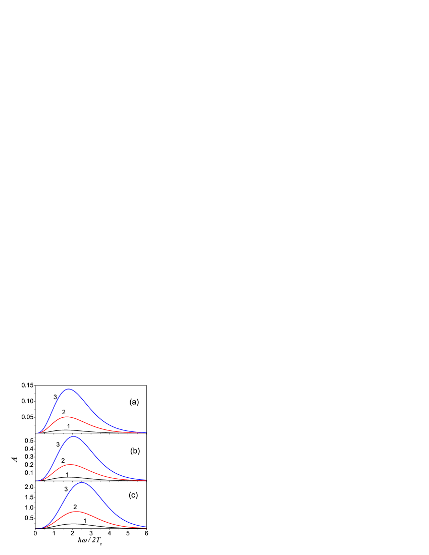
Figure 4: (Color online) The same as in Fig. 3 at $T_{c}=$600 K

For increasing temperatures the character of dependences from $n/\Delta n$ and $V_{g}$ is not modified, see Figs. 4a-c plotted for $T_{c}=$600 K. Here, for two times larger temperature the altitude of $A$ becomes about one order of magnitude smaller. However, as $G_{c}\propto T_{c}^{3}$, the maximal differential flows Eqs. (15) and (17) are weakely modified for such changes of $T_{c}$. In addition, point out that here the position of maximum is more strongly dependent on the character of generation-recombination processes than for the intrinsic graphene (compare Fig. 2 with Figs. 3 and 4).

III.3 Energy flow

Now, let us consider the integral energy flow for the cases (a) and (b), when Eqs. (7) and (10) can be expressed through the differential flow, Eq. (15). For the homogeneous case (a) the energy flow density takes form:

$$G_{\bot}=\frac{8\pi}{3}G_{c}\int\limits_{0}^{\infty}d\omega A\left(\frac{\hbar\omega}{2T_{c}}\right).$$ (18)

For intrinsic graphene at $T_{c}=$300 K we calculate from Eq. (18) that the flow $G_{\bot}\simeq$0.48 mW/cm², 2.02 mW/cm², and 4.69 mW/cm² corresponds, respectively, to $n/n_{T}=$0.5, 1, and 1.5; these $n/n_{T}$ are used in Fig. 2. For $T_{c}=$600 K and the same values of $n/n_{T}$, we obtain that the flow $G_{\bot}\simeq$ 7.68 mW/cm², 32.3 mW/cm², and 75.0 mW/cm².

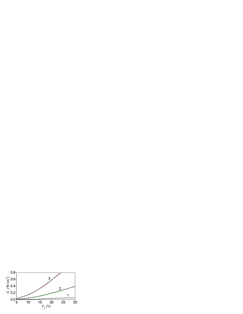
Figure 5: (Color online) Energy flow density $G_{\bot}$ versus $V_{g}$ for temperature $T_{c}=$300 K at at different generation-recombination levels determined by $n/\Delta n=$1.25 (1), 2 (2) and 3 (3). The dashed curves show the parabolic approximation, $G_{\bot}\propto V_{g}^{2}$.

Fig. 5 shows that for doped graphene $G_{\bot}$ increases for growing concentrations of carriers, defined by the gate voltage, whereas $n/\Delta n$ (or generation-recombination level) is fixed. From Fig. 5 it is seen that for $V_{g}\sim$20 V, which corresponds to the concentration of carriers $>2\times 10^{12}$ cm², the energy flow reaches the values $\sim 1$W/cm². In addition, the dependences $G_{\bot}$ versus $V_{g}$ are close to parabolic ones (see the dashed curves in Fig. 5). The temperature dependence of $G_{\bot}$ is weak (less than 10% for the $T_{c}$ increasing from 300 K to 600 K; pertinent graphs are not shown) because the spectral dependences are determined by dimensionless parameter $\hbar\omega/T_{c}$.

For the geometry (b) the radial component of energy flow in the far-zone Eq. (10) is expressed through $G_{\bot}$ as

$$G_{r}(\theta)=\frac{3S_{1}}{8\pi R^{2}}G_{\bot}\left(1+\cos^{2}\theta\right).$$ (19)

Here the angular dependence coincides with that of Eq. (15) and the energy flow (19) decreases $\propto R^{-2}$. Due to this, on macroscopic distances, for $\sqrt{S_{1}/R^{2}}\sim 10^{-3}$, it is possible to register the energy flow $\sim 1\mu$W/cm², while $G_{\bot}\sim 1$W/cm² is rather easily achievable according to the above treatment.

IV Discussion and concluding remarks

Summazing the consideration performed, the examination of luminescence caused by the interband transitions of hot electrons is presented. It is found, that the universal frequency-independent polarization of emission is realized for a weakly anisotropic distributions of nonequilibrium carriers. The spectral dependences of radiation are determined by the factor $\propto\omega^{3}$ multiplied by the product of electron and hole distributions. These data, together with measurements of the angular dependences and the integral intensity of radiation (the latter strongly depends on generation-recombination processes), allows the effective characterization of hot carriers. In addition, obtained efficient emission of hot carriers in mid-IR spectral regions opens a possibility for using the electroluminescence of graphene as a source of radiation.

Now let us discuss recent experiments on emission by hot carriers from the back-gated transistor structures, subjected to a strong in-plane electric field, 14 where measured spectral dependences are interpreted by using the Planck’s law. For the latter the high frequency asymptotic coincides with the asymptotic of Eq. (16), for the case of the quasiequilibrium Fermi distributions. From these spectral dependences in 14 it was found the relation of $T_{c}$ with a power of the Joule heating. However, the character of recombination, that could be determined from the intensity of radiation, was not investigated; dependences on a size of sample, angular dependences and polarization characteristics of the radiation also need a special treatment.

Next, we list and discuss the assumptions used. In the study of interaction of a radiation with the graphene sheet the only simplification used is the neglect by attenuation of radiation propagated along the layer, so that obtained results are not applicable for $\theta\to\pi/2$. More rigid constraint is imposed by modeling of the distributions of nonequilibrium carriers via the quasiequilibrium Fermi functions, with given effective temperature and concentrations of carriers. This approximation shows that important information on the mechanisms of energy relaxation and recombination can be obtained from the spectra of luminescence. However, for more precise calculation of the spectral dependences more realistic distribution functions of carriers will be needed. Further, the spectral and the polarization dependences can be separated only in an approximation of a weak anisotropy of the distribution of carriers. But such a separation can be broken under a strong enough electric field when an essential anisotropy of the distribution functions appears.

We also have restricted our consideration by the homogeneous geometry (without taking into account of the edge effects) and the far-zone region geometry [approaches (a) and (b) in Figs. 1a and 1b], however, the general treatment implies solving of Eqs(1), (2) for a specific geometry that is not well enough approximated by any of these two limit geometries.

To conclude, obtained results show that spectral, angular, and polarization dependences of the electroluminescence provide a convenient method of characterization of the hot carriers in graphene (along with the electrooptical measurements 15 and a study of the Raman scattering 14 ; 16 ). Therefore present results will stimulate subsiquent experiments and their theoretical interpretations designated for a verification of the relaxation mechanisms of nonequilibrium carriers under their heating both for the electric field and for the interband photoexcitation.

References

- (1) P.Y. Yu and M. Cardona, Fundamentals of Semiconductors, 4th ed. (Springer, Berlin 2010); J. I. Pankove, Optical Processes in Semiconductors (Prentice-Hall, New Jersey, 1971).
- (2) R. Cingolani and K. Ploog, Adv. Phys. 40, 535 (1991); F. T. Vasko and A. V. Kuznetsov, Electron States and Optical Transitions in Semiconductor Heterostructures (Springer, New York, 1998).
- (3) S. Komiyama, Adv. Phys. 31, 255 (1982); A. A. Andronov, Fiz. Tekh. Poluprov., 21, 1153 (1987) [Sov. Phys. Semicond. 21, 701 (1987)].
- (4) J. Moser, A. Barreiro, and A. Bachtold, Appl. Phys. Lett. 91, 163513 (2007); I. Meric, M. Y. Han, A. F. Yang, B. Ozyilmaz, P. Kim, and K. L. Shepard, Nature Nanotech. 3, 654 (2008); A. Barreiro, M. Lazzeri, J. Moser, F. Mauri, and A. Bachtold, Phys. Rev. Lett. 103, 076601 (2009).
- (5) O.G. Balev, F.T. Vasko and V. Ryzhii, Phys. Rev. B 76, 1654432 (2009); O.G. Balev and F.T. Vasko, J. Appl. Phys. 107, 124312 (2010).
- (6) A. Akturka and N. Goldsman, J. Appl. Phys. 103, 053702 (2008); R. S. Shishir and D. K. Ferry, J. Phys.: Condens. Matter, 21, 344201 (2009); V. Perebeinos and P. Avouris, Phys. Rev. B. 81, 195442 (2010).
- (7) L.A. Falkovsky, Phys. Usp. 51, 887 (2008); T. Stauber, N. M. R. Peres, and A. K. Geim, Phys. Rev. B78, 085432 (2008).
- (8) F. T. Vasko and O. E. Raichev, Quantum Kinetic Theory and Applications (Springer, New York 2005).
- (9) F.T. Vasko, Sov. Phys.Solid State 30, 1207 (1988); F.T. Vasko, O.G. Balev, and P. Vasilopoulos, Phys. Rev. B 47, 16433 (1993); V.V. Mitin, G. Paulavicius, and N. A. Bannov, J. Appl. Phys. 79, 8955 (1996).
- (10) E.M. Lifshitz, L.P. Pitaevskii, and V.B. Berestetskii, Quantum Electrodynamics (Butterworth-Heinemann, 1982); P.R. Wallace, Phys. Rev. 71, 622 (1947).
- (11) A. H. Castro Neto, F. Guinea, N. M. R. Peres, K. S. Novoselov, and A. K. Geim, Rev. Mod. Phys. 81, 109 (2009).
- (12) L. D. Landau and E.M. Lifshitz, Theory of Field, (Butterworth-Heinemann, 1982).
- (13) To obtain Eq. (9) we have used the matrix elements of the Pauli matrices as follows: and .
- (14) S. Berciaud, M. Y. Han, L. E. Brus, P. Kim, and T.F. Heinz, arXiv: 1003.6101; M. Freitag, H.-. Chiu, M. Steiner, V. Perebeinos, and P. Avouris, arXiv: 1004.0369.
- (15) F. T. Vasko and M.V. Strikha, Phys. Rev. B 81, 115413 (2010).
- (16) M. Freitag, M. Steiner, Y. Martin, V. Perebeinos, Z. Chen, J. C. Tsang, and P. Avouris Nano Letters 9, 1883 (2009); D.-H. Chae, B. Krauss, K. von Klitzing, and J.H. Smet, Nano Letters 10, 466 (2010).