Optical homodyne detection in view of joint probability distribution

Abstract

Optical homodyne detection is examined in view of joint probability distribution. It is usually discussed that the relative phase between independent laser fields are localized by photon-number measurements in interference experiments such as homodyne detection. This provides reasoning to use operationally coherent states for laser fields in the description of homodyne detection and optical quantum-state tomography. Here, we elucidate these situations by considering the joint probability distribution and the invariance of homodyne detection under the phase transformation of optical fields.

I Introduction

Laser technology plays essential roles in a wide variety of fields in physics. Since the first observation of interference fringes between two independent laser fields Magyar1963 , it has been common to employ a coherent state Glauber1963

$$|\alpha\rangle=e^{-|\alpha|^{2}/2}\sum_{n=0}^{\infty}\frac{\alpha^{n}}{n!}|n\rangle$$ (1)

to describe the quantum state of a laser field, which involves a coherent superposition of photon number states $|n\rangle$ with a definite phase in the complex amplitude $\alpha$. This quantum coherence provides indispensable resources for quantum information and communication. On the other hand, it is widely accepted Sargent1974 ; Walls1994 that by considering the driving mechanism the steady state of field inside a laser cavity should be a mixed state as

$$\hat{\rho}_{|\alpha|}=e^{-|\alpha|^{2}}\sum_{n=0}^{\infty}\frac{|\alpha|^{2n}}{n!}|n\rangle\langle n|=\int\frac{d\varphi}{2\pi}|\alpha e^{i\varphi}\rangle\langle\alpha e^{i\varphi}|,$$ (2)

which has no coherence, lacking a definite phase. It is, however, shown by a numerical simulation Molmer1997 that two cavity fields without definite phases even exhibit interference when continuously monitored by photon detectors. This provides a typical example for the apparent relevance of the coherent state as the laser field. Then, there have been a lot of debates concerning the quantum state of laser and optical coherence (see Molmer1997 ; Rudolph2001 ; vanEnk2001 ; Sanders2003 ; Wiseman2004 ; Smolin2004 ; Cable2005 ; Neri2005 ; Bartlett2007 , and references therein). The essential problem is whether the use of the coherent state of Eq. (1) in various applications is valid or not instead of the mixed state of Eq. (2) inside the laser cavity.

In quantum optics with the rotating wave approximation, which is usually employed when describing matter-field interaction, one can implement only the photon-number measurement, without observing the absolute phases of fields. Then, the U(1) invariance appears naturally in quantum optics Sanders2003 , namely the photon number operator $\hat{n}=\hat{a}^{\dagger}\hat{a}$ of each optical mode is invariant under the phase transformation, $\hat{a}^{\dagger}\to\hat{a}^{\dagger}e^{i\varphi}$ and $\hat{a}\to\hat{a}e^{-i\varphi}$ for the creation and annihilation operators $\hat{a}^{\dagger}$ and $\hat{a}$, respectively, inducing $|\alpha\rangle\to|\alpha e^{i\varphi}\rangle$ for the coherent state. This phase transformation has intimate relation to the fact that the phase of a single mode solely has no physical relevance, i.e., there is no absolute reference frame for the optical phases Bartlett2007 . In this sense, it is trivial that there appears no significant difference between the coherent state of Eq. (1) and the mixed state of Eq. (2) as long as U(1)-invariant operations and measurements are performed starting only with a single-mode optical field.

The real issue to be clarified is rather the interference between two independent optical fields, which are mutually incoherent without definite phases as seen in Eq. (2). It has been discussed that photon-number measurements induce localization of the relative phase when two mutually incoherent fields interfere Sanders2003 ; Cable2005 ; Neri2005 . Actually, after many photons are detected in an interference experiment, the relative phase is eventually localized around a certain value, and the remaining state gets projected to have a some definite relative phase. Thus, the later measurement outcomes exhibit an interference pattern.

The aim of this paper is to elucidate these situations in optical interference experiments, where laser fields are treated operationally as coherent states. Specifically, we consider homodyne detection and quantum-state tomography. In order to illustrate the apparent relevance for the use of coherent states, we consider the joint probability distribution of the measurement outcomes and the resultant empirical measure determining the quadrature distribution. In this examination we adopt the proper description of the output field of laser vanEnk2001 . We also note that the homodyne detection or generally photon-number detections are invariant under the rotation of the phase frame over optical fields.

This paper is organized as follows. In Sec. II, we consider repeated homodyne detections for independent signal and local oscillator fields to see the localization of the relative phase. In Sec. III, we introduce the joint probability distribution of the outcomes of the homodyne detections, and discuss the apparent relevance to use the coherent state as the laser field in the description of homodyne detection. In Sec. IV, we consider the optical quantum-state tomography based on these arguments on the homodyne detection, and examine the quantum states of laser fields. Sec. V is devoted to summary.

II Phase localization by homodyne detections

It has been argued Sanders2003 ; Cable2005 ; Neri2005 that the relative phase gets localized by measurements when two mutually incoherent fields interfere. Here, we consider the homodyne detection as a typical example of interference experiment to discuss the phase localization, which provides a reason why a coherent state may be adopted operationally for the local oscillator (LO) field as the reference.

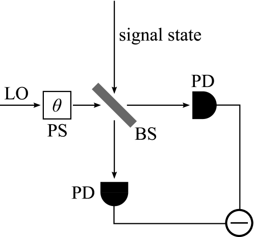
Figure 1: Schematic diagram of homodyne detection.

The homodyne detection is a scheme to measure the field quadratures and their probability distribution (see Fig. 1). A signal field and a local oscillator are injected together into a 50:50 beam splitter, and then the difference of the photon counts in the output modes is measured. The quadrature of the signal field is given with a coherent state LO $|\alpha\rangle$ ($\alpha\equiv e^{i\theta}|\alpha|$) by

$$\hat{x}_{\theta}=(\hat{a}e^{-i\theta}+\hat{a}^{\dagger}e^{i\theta})/\sqrt{2},$$ (3)

which is approximately proportional to the photon-number difference $\Delta\hat{n}\simeq\sqrt{2}|\alpha|\hat{x}_{\theta}$ for $|\alpha|\gg 1$ Tyc2004 . This quantity is sensitive to the relative phase between the signal and LO.

In usual homodyne experiments, the signal and LO are derived from a common laser field to compensate the phase fluctuation. In such a case, the laser field can be regarded as a coherent state since its absolute phase, which is inherited equally by the signal and LO, is irrelevant (or unobservable) in the homodyne detection sensitive to the relative phase. Instead, we here consider the case where the signal and LO come from independent sources, which are thus mutually incoherent.

We adopt an ideal continuous-wave (CW) laser as the LO. The quantum state of the CW laser field is described properly according to a formalism in Ref. vanEnk2001 . [A pulsed-wave (PW) laser (not phase-locked one) will also be considered in Sec. IV to discuss the optical quantum-state tomography though the phase localization is unavailable for the PW case.] Specifically, the output field of laser is separated into a sequence of wave packet modes, each with the same duration. By assuming the mixed state as given in Eq. (2) for the field inside the laser cavity and the linear coupling between the modes inside and outside the cavity, the sequence of $N$ output packets is described as

$$\hat{\rho}_{\text{CW}}=\int\frac{d\varphi}{2\pi}P(\varphi)\left(|\alpha e^{i\varphi}\rangle\langle\alpha e^{i\varphi}|\right)^{\otimes N},$$ (4)

where $\alpha>0$ is determined in terms of the field intensity inside the cavity, the cavity leakage rate and the packet duration. This is a mixture of tensor products of coherent states over their unknown phases. Here, the phase distribution $P(\varphi)$ is introduced generally, which may be non-uniform, while the Poissonian photon-number distribution is maintained. As discussed in Ref. vanEnk2001 , this form for the output state of laser is exchangeable among the packets to meet the quantum de Finetti theorem Hudson1976 ; Caves2002 . The phase distribution changes apparently as $P(\varphi)\to P(\varphi-\theta)$ under the phase rotation $\mathcal{U}_{\theta}\hat{\rho}_{\text{CW}}\mathcal{U}_{\theta}^{\dagger}$.

We may take a tensor product of $N$ packets as $\hat{\rho}^{\otimes N}$ for the signal field. That is, many identical copies of $\hat{\rho}$ are prepared and measured repeatedly in the homodyne detection. Then, the initial state of the system is given by

$$\hat{\rho}^{\otimes N}\otimes\hat{\rho}_{\text{CW}}=\int\frac{d\varphi}{2\pi}P(\varphi)\left(\hat{\rho}\otimes|\alpha e^{i\varphi}\rangle\langle\alpha e^{i\varphi}|\right)^{\otimes N}.$$ (5)

[Similar argument is also applicable for a phase-mixture signal, as given in Eq. (4), as long as the relative phase between the signal and LO is concerned. This case will be considered explicitly in Sec. IV.] After the first packet is measured, the remaining packets are projected to

$$\int\frac{d\varphi}{2\pi}P(\varphi)q_{\varphi}(x)\left(\hat{\rho}\otimes|\alpha e^{i\varphi}\rangle\langle\alpha e^{i\varphi}|\right)^{\otimes(N-1)}$$ (6)

up to the normalization. The quadrature value $x$ is determined from the detected photon-number difference $\Delta n$ by

$$x=\Delta n/(\sqrt{2}\alpha).$$ (7)

The quadrature distribution $q_{\varphi}(x)$ for the signal $\hat{\rho}$ with a pure coherent state LO $|\alpha e^{i\varphi}\rangle$ is given by

$$\frac{q_{\varphi}(x)[\hat{\rho}]}{\sqrt{2}\alpha}=\sum_{n-m=\Delta n}\langle n,m|\mathcal{B}\left[\hat{\rho}\otimes|\alpha e^{i\varphi}\rangle\langle\alpha e^{i\varphi}|\right]|n,m\rangle,$$ (8)

where $\mathcal{B}$ represents the unitary transformation by the 50:50 beam splitter. Specifically, for the strong LO field we have approximately Tyc2004

$$q_{\varphi}(x)=\langle{\hat{x}_{\varphi}=x}|\hat{\rho}|{\hat{x}_{\varphi}=x}\rangle\quad(\alpha\to\infty),$$ (9)

where $|{\hat{x}_{\varphi}=x}\rangle$ is an eigenstate of the quadrature $\hat{x}_{\varphi}$ with an eigenvalue $x$.

Repetition of $M$ detections with outcomes $x_{1},\ldots,x_{M}$ leads the state of the LO field to be

$$\int\frac{d\varphi}{2\pi}\left[P(\varphi)\prod_{i=1}^{M}q_{\varphi}(x_{i})\right]\left(|\alpha e^{i\varphi}\rangle\langle\alpha e^{i\varphi}|\right)^{\otimes(N-M)}.$$ (10)

Typically, for a coherent state signal $\hat{\rho}=|\beta\rangle\langle\beta|$ ($\beta>0$) we have the quadrature distribution ($\alpha\to\infty$)

$$q_{\varphi}(x)=\frac{1}{\sqrt{\pi}}\exp\left[-2\beta^{2}\left(\cos\varphi-\frac{x}{\sqrt{2}\beta}\right)^{2}\right].$$ (11)

Then, the phase distribution of the LO field after the $M$ detections is modified from $P(\varphi)$ by the factor

$$\prod_{i=1}^{M}q_{\varphi}(x_{i})\propto\left\{\exp\left[-2\beta^{2}\left(\cos\varphi-\frac{\bar{x}_{M}}{\sqrt{2}\beta}\right)^{2}\right]\right\}^{M},$$ (12)

where $\bar{x}_{M}$ is the average over the $M$ outcomes. This provides a sharp Gaussian distribution around $\cos\varphi=\bar{x}_{M}/(\sqrt{2}\beta)$ with the standard deviation $1/(2\beta\sqrt{M})$ for $M\gg 1$. That is, the phase of the LO field gets localized to $\varphi_{0}=\pm\arccos(\bar{x}_{M}/\sqrt{2}\beta)$ by the repeated homodyne detections. Generally, as long as $q_{\varphi}(x)$ is non-uniform with respect to the phase $\varphi$ of the LO (more precisely the relative phase between the signal and LO), the phase localization takes place after a large number of detections as (up to the normalization)

$$\prod_{i=1}^{M}q_{\varphi}(x_{i})\approx\delta(\varphi-\varphi_{0}).$$ (13)

The phase localization is usually discussed in the case of single measurement ($M=1$) with detection of large numbers of photons under strong sources ($\alpha,\beta\to\infty$) Sanders2003 ; Cable2005 ; Neri2005 . Here, we note that the phase localization takes place by repeated measurements ($M\gg 1$) even for the source packets with weak amplitudes ($\alpha,\beta\sim 1$). This indeed provides a process of aligning the reference frames between the signal and LO Bartlett2007 by updating the relative phase according to the Bayesian rule in Eq. (10) vanEnk2001 ; Buzek1998 ; Schack2001 ; Neri2005 . The localized phase $\varphi_{0}$ may apparently take multiple values, reflecting a specific symmetry of the signal state, though they are physically equivalent. For example, in the case of $\hat{\rho}=|\beta\rangle\langle\beta|$ we have $\varphi_{0}=\pm\arccos(\bar{x}_{M}/\sqrt{2}\beta)$ for $q_{\varphi}(x)=q_{-\varphi}(x)$ under the phase reflection $\varphi\to-\varphi$.

Once the phase of the LO field is localized to a particular value $\varphi_{0}$ in Eq. (13), the state of the LO field conditioned on the outcomes $x_{1},\ldots,x_{M}$ gets projected as

$$\hat{\rho}_{\text{CW}}^{(x_{1},\ldots,x_{M})}\approx\left(|\alpha e^{i\varphi_{0}}\rangle\langle\alpha e^{i\varphi_{0}}|\right)^{\otimes(N-M)}.$$ (14)

Thus, we may conclude that the pure coherent state $|\alpha e^{i\varphi_{0}}\rangle$ is provided as the LO for the subsequent detections in the same way as the usual homodyne detection. The apparent exception of the phase localization is the case that the signal state $\hat{\rho}$ is invariant under the phase transformation, including the number states and their mixtures. Nevertheless, the quadrature distributions for such a state with the pure coherent state LO $|\alpha e^{i\varphi}\rangle$ in Eq. (1) and the mixed state LO in Eq. (2) are identical as $q_{\varphi}(x)=q(x)$ independently of $\varphi$. Thus, even in this case without phase localization, the laser field can be regarded as the coherent state. This point will be clarified further in view of the joint probability distribution in the following sections.

III Joint probability distribution in homodyne detections

We have seen that after repeated detections, the state of the LO field turns into the product of coherent states in Eq. (14) due to the phase localization. This provides reasoning to use the coherent state in the standard description of homodyne detection. In order to get further understanding of this point from a viewpoint of probability theory, we here consider the joint probability distribution of homodyne detections.

In quantum theory, measurements of a physical quantity yield probabilistic outcomes. Then, from the relative frequency of outcomes we can infer the probability distribution for the physical quantity. This argument is based on the assumption that the outcomes are independent and identically distributed (i.i.d.) in repeated measurements for an ensemble of identically prepared quantum states. Specifically, in the optical quantum-state tomography Lvovsky2009 the quadrature distributions are determined from the outcomes of homodyne detections. In the standard description, a product of pure coherent states $\left(|\alpha e^{i\varphi_{0}}\rangle\langle\alpha e^{i\varphi_{0}}|\right)^{\otimes N}$ with a common phase $\varphi_{0}$ is adopted as the LO packets when the homodyne detections are performed repeatedly for an ensemble of signal states as $\hat{\rho}^{\otimes N}$. Then, the joint probability distribution of the outcomes $x_{1},\ldots,x_{M}$ is given by

$$p(x_{1},\ldots,x_{M})=\prod_{i=1}^{M}q_{\varphi_{0}}(x_{i}),$$ (15)

where $q_{\varphi_{0}}(x)$ is the quadrature distribution of the signal in Eq. (8). In this case the outcomes are really i.i.d., namely they are obtained probabilistically according to the product of identical quadrature distributions. Thus, owing to the Glivenko-Cantelli theorem the original distribution $q_{\varphi_{0}}(x)$ is properly inferred as the relative frequency of outcomes for $M\to\infty$.

This argument for the standard homodyne detection with the pure coherent state LO can be extended for the case of the real output field of a CW laser whose quantum state is the mixture as given in Eq. (4). The (unnormalized) state of the LO field after $M$ detections is given in Eq. (10). By tracing out the remaining packets as $\operatorname{Tr}\left[(|\alpha e^{i\varphi}\rangle\langle\alpha e^{i\varphi}|)^{\otimes(N-M)}\right]=1$, the joint probability distribution of the outcomes is calculated as

$$p(x_{1},\ldots,x_{M})=\int\frac{d\varphi}{2\pi}P(\varphi)\prod_{i=1}^{M}q_{\varphi}(x_{i}).$$ (16)

Even in this extended case, where the joint probability distribution in Eq. (16) appears as a phase-mixture of the i.i.d. products in Eq. (15), we can infer the original quadrature distributions from the measurement outcomes as described in the following.

Consider a sequence of random real variables (measurement outcomes),

$$\tilde{x}_{M}\equiv(x_{1},x_{2},\ldots,x_{M}).$$ (17)

The empirical measure $\Lambda_{\tilde{x}_{M}}$, or relative frequency of the $M$ outcomes, is defined as a probability measure on $\mathbb{R}$ by

$$\Lambda_{\tilde{x}_{M}}=\frac{1}{M}\sum_{i=1}^{M}\delta_{x_{i}},$$ (18)

where $\delta_{x}$ denotes the Dirac measure on $\mathbb{R}$:

$$\delta_{x}(A)=\begin{cases}1&\text{if $x\in A\subset\mathbb{R}$,}\\ 0&\text{otherwise.}\end{cases}$$ (19)

That is, if the number of $x_{i}$’s which have values in $A$ is $k$, then $\Lambda_{\tilde{x}_{M}}(A)=k/M$. In the i.i.d. case of Eq. (15), the Glivenko-Cantelli theorem ensures that the empirical measure $\Lambda_{\tilde{x}_{M}}$ converges to the original distribution $q_{\varphi_{0}}(x)$ for $M\to\infty$. As for the actual homodyne detection with the LO of a CW laser field, the joint probability distribution in Eq. (16) represents a mixture of the i.i.d. variables (or i.i.d.’s shortly). Even in this case, by repeating the detection many times ($M\gg 1$) the empirical measure provides the quadrature distribution with a certain random phase $\varphi_{0}$,

$$\lim_{M\to\infty}\Lambda_{\tilde{x}_{M}}(x)=q_{\varphi_{0}}(x)$$ (20)

(see Ref. Aldous1985 for the mathematical details). This implies that the outcomes $x_{1},\ldots,x_{M}$ appear as if they were i.i.d., in the same way as the case with the pure coherent state LO. Therefore, in each sequence of homodyne detections we may regard the LO of the CW laser field as a coherent state $|\alpha e^{i\varphi_{0}}\rangle$ while the phase $\varphi_{0}$ is determined a posteriori by the localization.

We have made numerical simulations for the joint probability distributions of homodyne detections, confirming Eq. (20). A sequence of $M$ outcomes are obtained according to Eq. (16) representing the mixture of i.i.d.’s. Specifically, the $i$-th outcome $x_{i}$ is generated under the conditional probability distribution,

$$p(x_{i}|x_{1},\ldots,x_{i-1}) = \frac{p(x_{1},\ldots,x_{i})}{p(x_{1},\ldots,x_{i-1})}$$ (21)

$$= \int\frac{d\varphi}{2\pi}P_{(x_{1},\ldots,x_{i-1})}(\varphi)q_{\varphi}(x_{i})$$

with

$$p(x_{1},\ldots,x_{i})=\int dx_{i+1}\cdots dx_{M}p(x_{1},\ldots,x_{M}).$$ (22)

(A similar analysis is made for the spatial interference of Bose-Einstein condensates Javanainen1996 .) Here, the phase distribution is updated by the Bayesian rule vanEnk2001 ; Buzek1998 ; Schack2001 ; Neri2005 upon the preceding quadrature outcomes $x_{1},\ldots,x_{i-1}$ as

$$P_{(x_{1},\ldots,x_{i-1})}(\varphi)=\prod_{j=1}^{i-1}q_{\varphi}(x_{j})\left/\int\frac{d\varphi}{2\pi}\prod_{j=1}^{i-1}q_{\varphi}(x_{j})\right.$$ (23)

with the U(1)-invariant initial $P(\varphi)=1$ for definiteness. The empirical measure $\Lambda_{\tilde{x}_{M}}(x)$ is then calculated from the $M$ outcomes with Eq. (18). In this numerical analysis, the original quadrature distribution $q_{\varphi}(x)$ is calculated precisely from Eq. (8) without taking the limit of strong laser intensity. Statistically, a large number of detections should be made to infer the quadrature distribution. Thus, we realize in Eq. (23) that in the early portion of the $M$ detections ($M\gg 1$) the phase $\varphi$ is almost localized to $\varphi_{0}$ providing Eq. (20).

Figure 2: Typical results of the empirical measure $\Lambda_{\tilde{x}_{M}}(x)$ (solid lines) are shown for the squeezed state signal $\hat{\rho}=|r,\beta\rangle\langle r,\beta|$, where $M=10000$ outcomes are generated for each operation of repeated homodyne detections. The parameters for the LO and signal is taken as $\alpha=\sqrt{15}$, $\beta e^{-r}={\sqrt{3}}$ and $r=-1$. The resolution of the quadrature is given by $\Delta x=1/(\sqrt{2}\alpha)=1/\sqrt{30}$. The resultant random phases $\varphi_{0}$ are estimated from the average $\bar{x}_{M}$ of the outcomes as $\varphi_{0}=3.05\,\text{rad}$, $1.94\,\text{rad}$, $0.43\,\text{rad}$ from the left to right. The quadrature distributions $q_{\varphi_{0}}(x)$ (dashed lines) are also plotted for these values of $\varphi_{0}$, showing good agreement with $\Lambda_{\tilde{x}_{M}}(x)$.

Fig. 2 shows typical results of the empirical measure $\Lambda_{\tilde{x}_{M}}(x)$ (solid lines) for the squeezed state signal $\hat{\rho}=|r,\beta\rangle\langle r,\beta|$, where $M=10000$ outcomes are generated for each operation of repeated homodyne detections. The parameters for the LO and signal is taken as $\alpha=\sqrt{15}$, $\beta e^{-r}={\sqrt{3}}$ and $r=-1$. The resolution of the quadrature $x$ is given by $\Delta x=1/(\sqrt{2}\alpha)$ in Eq. (7) with $\Delta n=1$. We note that the expectation value of the quadrature is calculated with $q_{\varphi}(x)$ as $\sqrt{2}\beta e^{-r}\cos\varphi$ independently of $\alpha>0$ for the coherent state LO. Since it should agree with the average $\bar{x}_{M}$ of the outcomes for $M\to\infty$, the resultant random phases $\varphi_{0}$ are estimated as $\varphi_{0}=3.05\,\text{rad}$, $1.94\,\text{rad}$, $0.43\,\text{rad}$ from the left to right in Fig. 2. Then, the quadrature distributions $q_{\varphi_{0}}(x)$ (dashed lines) are plotted for these values of $\varphi_{0}$ for comparison. These results really show good agreement of $\Lambda_{\tilde{x}_{M}}(x)$ and $q_{\varphi_{0}}(x)$, as expected in Eq. (20).

IV Optical quantum-state tomography

In the view of joint probability distribution for homodyne detection, as described in the previous section, we now consider the optical quantum-state tomography, and discuss the quantum state of a laser field. The signal state (e.g., Wigner function) is reconstructed from the quadrature distributions $q_{\theta}(x)$ for various phase shifts $\theta$, which are obtained as the empirical measures from the outcomes of homodyne detections. The change of $\theta$ is realized by applying a phase shifter on the LO.

IV.1 Tomography with a common source oscillator

We first consider the usual setup for optical tomography, where the signal and LO are supplied by splitting a single oscillator, as done in many actual experiments. The output state of a CW laser for the original oscillator ($\alpha,\beta>0$) is given as

$$\hat{\rho}_{\text{CW}}^{0}=\int\frac{d\varphi}{2\pi}P(\varphi)\left[|(\alpha+\beta)e^{i\varphi}\rangle\langle(\alpha+\beta)e^{i\varphi}|\right]^{\otimes N}.$$ (24)

The signal and LO, which share the common random phase $\varphi$, are derived from this laser field as

$$\hat{\rho}_{\text{CW}}^{\text{SL}}=\int\frac{d\varphi}{2\pi}P(\varphi)\left[\hat{\rho}(\varphi)\otimes|\alpha e^{i(\varphi+\theta)}\rangle\langle\alpha e^{i(\varphi+\theta)}|\right]^{\otimes N}$$ (25)

with

$$\hat{\rho}(\varphi)=\mathcal{E}|\beta e^{i\varphi}\rangle\langle\beta e^{i\varphi}|\mathcal{E}^{\dagger}=\mathcal{U}_{\varphi}\hat{\rho}(0)\mathcal{U}_{\varphi}^{\dagger}.$$ (26)

Here, the phase of the LO is shifted by $\theta$, and the operation $\mathcal{E}$ such as squeezing is applied for the signal, which commutes with the phase transformation $\mathcal{U}_{\varphi}$. We see below that this setup reproduces the standard description of homodyne tomography with a pure coherent state $|\alpha\rangle$ as the LO. The joint probability distribution of the quadrature outcomes $(x_{1},\ldots,x_{M})\equiv\tilde{x}_{M}$ ($M\gg 1$) for $M$ packets is calculated as

$$p(\tilde{x}_{M})[\hat{\rho}_{\text{CW}}^{\text{SL}}] = \int\frac{d\varphi}{2\pi}P(\varphi)\prod_{i=1}^{M}q_{\varphi+\theta}(x_{i})[\hat{\rho}(\varphi)]$$ (27)

$$= \prod_{i=1}^{M}q_{\theta}(x_{i})[\hat{\rho}(0)].$$

Here, we have considered the fact that the homodyne detection is an invariant operation under the simultaneous phase rotation $\mathcal{U}_{\varphi}$ for the signal and LO as $|\alpha e^{i(\varphi+\theta)}\rangle\to|\alpha e^{i\theta}\rangle$ and $|\beta e^{i\varphi}\rangle\to|\beta\rangle$, which implies

$$q_{\varphi+\theta}(x)[\hat{\rho}(\varphi)]=q_{\theta}(x)[\hat{\rho}(0)],$$ (28)

i.e., it is sensitive only to the relative phase $\theta$. This $p(\tilde{x}_{M})$ turns out to be independent of the phase distribution $P(\varphi)$ for the LO, that is the possible U(1) violation in the laser field is not observable in this scheme. The quadrature outcomes are i.i.d. in Eq. (27), and the LO appears as if it is the coherent state $|\alpha e^{i\theta}\rangle$ with $\varphi=0$. Thus, by repeating independently the sequence of $M$ detections on $\hat{\rho}_{\text{CW}}^{\text{SL}}$ from the common source with the varying phase shift $\theta$ for the LO, the set of quadrature distributions $q_{\theta}(x)[\hat{\rho}(0)]$ is obtained to reconstruct the signal state through tomography as

$$\hat{\rho}_{\text{rec}}=\hat{\rho}(0)=\mathcal{E}(|\beta\rangle\langle\beta|)\mathcal{E}^{\dagger},$$ (29)

which is irrespective of the unknown phase $\varphi$.

Alternatively, we may adopt a PW laser for the original oscillator, providing $N$ copies of a phase-mixture of coherent states,

$$\hat{\rho}_{\text{PW}}^{0}=\left[\int\frac{d\varphi}{2\pi}P(\varphi)|(\alpha+\beta)e^{i\varphi}\rangle\langle(\alpha+\beta)e^{i\varphi}|\right]^{\otimes N}.$$ (30)

The combination of signal and LO is derived as

$$\hat{\rho}_{\text{PW}}^{\text{SL}}=\left[\int\frac{d\varphi}{2\pi}P(\varphi)\hat{\rho}(\varphi)\otimes|\alpha e^{i(\varphi+\theta)}\rangle\langle\alpha e^{i(\varphi+\theta)}|\right]^{\otimes N}.$$ (31)

Then, the same joint probability distribution is obtained as Eq. (27) for the CW case,

$$p(\tilde{x}_{M})[\hat{\rho}_{\text{PW}}^{\text{SL}}] = \prod_{i=1}^{M}\int\frac{d\varphi_{i}}{2\pi}P(\varphi_{i})q_{\varphi_{i}+\theta}(x_{i})[\hat{\rho}(\varphi_{i})]$$ (32)

$$= \prod_{i=1}^{M}q_{\theta}(x_{i})[\hat{\rho}(0)],$$

providing again the reconstruction of the signal state as $\hat{\rho}(0)=\mathcal{E}(|\beta\rangle\langle\beta|)\mathcal{E}^{\dagger}$. Therefore, as long as the common laser field is used for the signal and LO, we find no actual difference between the CW and PW cases. In either case, the use of a pure coherent state as the LO is relevant for the standard description of the optical quantum-state tomography, without need to discuss the phase localization. The tomography with the common source just characterizes the process given by the operation $\mathcal{E}$ rather than the signal state Sanders2003 .

IV.2 Tomography with independent signal and LO

We next consider the case that the signal and LO are prepared independently, which may be more faithful in the sense of tomography to reconstruct an “unknown” quantum state. The LO is supplied with the output state $\hat{\rho}_{\text{CW}}$ of a CW laser as given in Eq. (4). An ensemble of repeatedly prepared identical states for the signal may be given generally as

$$\hat{\rho}_{\text{S}}=\int\frac{d\varphi^{\prime}}{2\pi}P_{\text{S}}(\varphi^{\prime})\hat{\rho}(\varphi^{\prime})^{\otimes N},$$ (33)

where

$$\hat{\rho}(\varphi^{\prime})\equiv\mathcal{U}_{\varphi^{\prime}}\hat{\rho}(0)\mathcal{U}_{\varphi^{\prime}}^{\dagger}$$ (34)

with certain $\hat{\rho}(0)$. The phase distributions $P(\varphi)$ and $P_{\text{S}}(\varphi^{\prime})$ (with period $2\pi$) may not be invariant under the rotation of phase frame. In the case of a U(1)-invariant state $\hat{\rho}(0)=\hat{\rho}(\varphi^{\prime})$ for any $\varphi^{\prime}$, namely a mixture of number states Sanders2003 , we simply have $\hat{\rho}_{\text{S}}=\hat{\rho}(0)^{\otimes N}$ without $P_{\text{S}}(\varphi^{\prime})$.

The joint probability distribution of homodyne detections is calculated as

$$p(\tilde{x}_{M})[\hat{\rho}_{\text{S}}\otimes\hat{\rho}_{\text{CW}}]=\int\frac{d\varphi}{2\pi}\bar{P}_{\text{S}}(\varphi)\prod_{i=1}^{M}q_{\varphi}^{(0)}(x_{i})$$ (35)

with a convoluted phase distribution

$$\bar{P}_{\text{S}}(\varphi)=\int\frac{d\varphi^{\prime}}{2\pi}P_{\text{S}}(\varphi^{\prime})P(\varphi+\varphi^{\prime}).$$ (36)

Here, we have considered the invariance of homodyne detection under the phase transformation, implying the relation for the quadrature distributions as

$$q_{\varphi}(x)[\hat{\rho}(\varphi^{\prime})]\equiv q_{\varphi}^{(\varphi^{\prime})}(x)=q_{\varphi-\varphi^{\prime}}^{(0)}(x)$$ (37)

with the periodicity $q_{\varphi+2\pi}(x)=q_{\varphi}(x)$. We find that this $p(\tilde{x}_{M})$ represents a mixture of i.i.d.’s, as discussed in Sec. III. Then, a quadrature distribution $q_{\varphi_{0}}^{(0)}(x)$ is obtained as the empirical measure with the probability distribution $\bar{P}_{\text{S}}(\varphi_{0})$ for the random phase $\varphi_{0}$. Here, we note that the U(1)-invariant LO with $P(\varphi)=1$ provides $\bar{P}_{\text{S}}(\varphi)=1$, irrespective of any $P_{\text{S}}(\varphi)$ for the original signal. Contrarily, if any deviation of $\bar{P}_{\text{S}}(\varphi)$ from the uniform distribution is found for the various values of $\varphi=\varphi_{0}$ in experiments (provided $\varphi_{0}$ is determined in a certain situation, e.g., from the average of outcomes for the coherent or squeezed state signal), that is

$$\bar{P}_{\text{S}}(\varphi)\neq 1\rightarrow P(\varphi),P_{\text{S}}(\varphi)\neq 1,$$ (38)

then it might indicate the violation of U(1) symmetry, or the presence of some implicit phase reference common to the signal and LO.

The measurement of the $M$-packet sequence may be repeated independently. Then, the quadrature distributions $q_{\varphi_{0}}^{(0)}(x)$ are obtained with various random phases $\varphi_{0}$. It is, however, impossible in general to know the actual values of $\varphi_{0}$ without some prior knowledge about the signal state. These unknown random phases $\varphi_{0}$ for $q_{\varphi_{0}}^{(0)}(x)$ thus can not substitute for the phase shift $\theta$ of the LO in tomography. The phase shift $\theta$ of the LO in each of the independent $M$-packet sequences is actually ineffective since it is hidden in the random phase $\varphi_{0}$.

Instead, in order to realize effectively the phase shift of the LO, we should extend the single $M$-packet sequence to $K\times M$-packet sequences in a single operation of tomography:

$$\hat{\rho}_{\text{CW}}\rightarrow\int\frac{d\varphi}{2\pi}P(\varphi)\prod_{k=1}^{K}\left[\left(|\alpha e^{i(\varphi+\theta_{k})}\rangle\langle\alpha e^{i(\varphi+\theta_{k})}|\right)^{\otimes M}\right],$$ (39)

where the phase shift $\theta_{k}$ is applied for the LO in each $M$-packet sequence. Then, the joint probability distribution is given as

$$p(\tilde{x}_{M}^{(1)},\ldots,\tilde{x}_{M}^{(K)})=\int\frac{d\varphi}{2\pi}\bar{P}_{\text{S}}(\varphi)\prod_{k=1}^{K}\left[\prod_{i=1}^{M}q_{\varphi+\theta_{k}}^{(0)}(x_{i})\right].$$ (40)

This provides the sequence of empirical measures upon homodyne detections, determining the quadrature distributions for tomography with varying phases $\theta_{k}$ ($M\gg 1$):

$$\Lambda_{\tilde{x}_{M}^{(1)}}=q_{\varphi_{0}+\theta_{1}}^{(0)}(x),\ldots,\Lambda_{\tilde{x}_{M}^{(K)}}=q_{\varphi_{0}+\theta_{K}}^{(0)}(x),$$ (41)

where the original phase of the LO is fixed to a certain value $\varphi_{0}$ according to the localization.

Provided there is no way to know the value of $\varphi_{0}$, we may set $\varphi_{0}=0$ operationally (as a convenient choice of the phase frame), or consider the relation

$$q_{\varphi_{0}+\theta_{k}}^{(0)}(x)=q_{\theta_{k}}^{(-\varphi_{0})}(x).$$ (42)

Then, the set of quadrature distributions $q_{\theta_{k}}^{(-\varphi_{0})}(x)$ for the pure coherent states LO $|\alpha e^{i\theta_{k}}\rangle$ with the phase shifts $\theta_{k}$ ($\alpha>0$ and $\varphi=0$) provides the tomographic reconstruction as

$$\hat{\rho}_{\text{rec}}=\hat{\rho}(-\varphi_{0}).$$ (43)

In each operation of tomography, the reconstructed state $\hat{\rho}(-\varphi_{0})$ appears probabilistically as a random rotation of $\hat{\rho}(0)$. Due to the lack of the absolute phase reference, however, $\hat{\rho}(0)$ and $\hat{\rho}(-\varphi_{0})$ should be regarded equivalent, and the ensemble of signal states is properly inferred as $\hat{\rho}_{\text{S}}$ in Eq. (33) with $\bar{P}_{\text{S}}(\varphi^{\prime})$. These arguments illustrate the actual relevance for the use of the pure coherent state as the LO in the description of optical quantum-state homodyne tomography. The random phases $\varphi_{0}$ and their distribution $\bar{P}_{\text{S}}(\varphi_{0})$ may be estimated relatively by comparing the rotations for the resultant Wigner functions obtained from many runs of tomography for the same $\hat{\rho}_{\text{S}}$. Note, however, that $\bar{P}_{\text{S}}(\varphi_{0})=1$ for the U(1)-invariant LO with $P(\varphi)=1$, irrespective of the actual $P_{\text{S}}(\varphi^{\prime})$.

IV.3 CW field versus PW field

We also consider the case that the quantum state of LO is given by a product of mixed states, which may be prepared with a simple PW laser (not a phase-locked one):

$$\hat{\rho}_{\text{PW}}=\left[\int\frac{d\varphi}{2\pi}P(\varphi)|\alpha e^{i\varphi}\rangle\langle\alpha e^{i\varphi}|\right]^{\otimes N}.$$ (44)

In the PW case as the LO, the joint probability distribution is calculated for the signal state in Eq. (33) as

$$p(\tilde{x}_{M})[\hat{\rho}_{\text{S}}\otimes\hat{\rho}_{\text{PW}}]=\int\frac{d\varphi^{\prime}}{2\pi}P_{\text{S}}(\varphi^{\prime})\prod_{i=1}^{M}\bar{q}_{\varphi^{\prime}}(x_{i}),$$ (45)

where

$$\bar{q}_{\varphi^{\prime}}(x)\equiv\int\frac{d\varphi}{2\pi}P(\varphi)q_{\varphi^{\prime}}^{(\varphi^{\prime}-\varphi+\varphi^{\prime})}(x).$$ (46)

with the relation $q_{\varphi}^{(\varphi^{\prime})}(x)=q_{\varphi^{\prime}}^{(\varphi^{\prime}-\varphi+\varphi^{\prime})}(x)$ under the phase rotation $\mathcal{U}_{-\varphi+\varphi^{\prime}}$. This smeared quadrature distribution $\bar{q}_{\varphi^{\prime}}(x)$ is reproduced with the LO state $|\alpha e^{i\varphi^{\prime}}\rangle$ for the signal of a phase-mixed state

$$\hat{\rho}_{\text{mix}}=\int\frac{d\varphi}{2\pi}P(\varphi)\hat{\rho}(\varphi^{\prime}-\varphi+\varphi^{\prime}),$$ (47)

which generally does not coincide with $\hat{\rho}(0)$ or its phase-rotation $\hat{\rho}(\varphi^{\prime})$, except for the U(1)-invariant $\hat{\rho}(0)$. Thus, we find that the optical quantum-state tomography does not work rightly by using the PW field $\hat{\rho}_{\text{PW}}$ in Eq. (44) as the independent LO. The phase-mixture of product coherent states $\hat{\rho}_{\text{CW}}$ in Eq. (4), which is derived from a CW laser, is required for the successful tomography. As an interesting case, we may implement the homodyne tomography for the CW and PW fields with the independent CW field as the LO. Then, we will obtain in the reconstruction the coherent state in Eq. (1) for the CW signal, and the mixed state in Eq. (2) for the PW signal, respectively. In this way, we can distinguish the quantum states of laser fields.

V Summary

We have examined the repeated optical homodyne detections and quantum-state tomography in view of the joint probability distribution of the measurement outcomes. By adopting the real output state of a CW laser as the LO, which is independent of the signal field, the joint probability distribution represents a mixture of i.i.d.’s. Then, the original quadrature distribution of the signal is obtained as the empirical measure, or relative frequency of the outcomes, with a random phase for the coherent state LO determined a posteriori by the phase localization according to the Bayesian rule. This justifies the operational use of the coherent state as the LO in the standard description of homodyne detection and tomography. We have also discussed that the quantum states of CW and PW lasers are distinguishable by the quantum-state tomography with the independent CW field as the LO. That is, the CW and PW lasers will appear as the coherent state and the mixed state, respectively. On the other hand, both of them will be recognized as the coherent state indistinguishably if the tomography is implemented with the signal and LO derived from the common source oscillator, as usually made in optical experiments.

- (1) G. Magyar and L. Mandel, Nature 198, 255 (1963).
- (2) R. J. Glauber, Phys. Rev. 131, 2766 (1963).
- (3) M. Sargent, III, M. O. Scully, and W. E. Lamb, Jr., Laser Physics (Addison-Wesley, Reading, 1974).
- (4) D. F. Walls and G. J. Milburn, Quantum Optics (Springer-Verlag, Berlin, 1994).
- (5) K. Mølmer, Phys. Rev. A 55, 3195 (1997); J. Mod. Opt. 44, 1937 (1997).
- (6) T. Rudolph and B. C. Sanders, Phys. Rev. Lett. 87, 077903 (2001).
- (7) S. J. van Enk and C. A. Fuchs, Phys. Rev. Lett. 88, 027902 (2001); Quant. Inf. Comput. 2, 151 (2002), arXiv:quant-ph/0111157.
- (8) B. C. Sanders, S. D. Bartlett, T. Rudolph, and P. L. Knight, Phys. Rev. A 68, 042329 (2003).
- (9) H. M. Wiseman, J. Opt. B 6, S849 (2004).
- (10) J. A. Smolin, arXiv:quant-ph/0407009.
- (11) H. Cable, P. L. Knight, and T. Rudolph, Phys. Rev. A 71, 042107 (2005).
- (12) F. Neri, Phys. Rev. A 72, 062306 (2005).
- (13) S. D. Bartlett, T. Rudolph, and R. W. Spekkens, Rev. Mod. Phys. 79, 555 (2007).
- (14) R. L. Hudson and G. R. Moody, Z. Wahrs. 33, 343 (1976).
- (15) C. M. Caves, C. A. Fuchs, and R. Schack, J. Math. Phys. 43, 4537 (2002); 49, 019902 (2008).
- (16) V. Bužek, R. Derka, G. Adam, and P. L. Knight, Ann. Phys. (NY) 266, 454 (1998).
- (17) R. Schack, T. A. Brun, and C. M. Caves, Phys. Rev. A 64, 014305 (2001).
- (18) T. Tyc and B. C. Sanders, J. Phys. A 37, 7341 (2004).
- (19) D. J. Aldous, in École d’Été de Probabilités de Saint-Flour XIII — 1983, Lecture Notes in Mathematics, Vol. 1117, edited by P. L. Hennequin (Springer-Verlag, Berlin, 1985) pp. 1–198.
- (20) A. I. Lvovsky and M. G. Raymer, Rev. Mod. Phys. 81, 299 (2009), and references therein.
- (21) J. Javanainen and S. M. Yoo, Phys. Rev. Lett. 76, 161 (1996).