Ehrenfest-time Dependence of Counting Statistics for Chaotic Ballistic Systems

Abstract

Transport properties of open chaotic ballistic systems and their statistics can be expressed in terms of the scattering matrix connecting incoming and outgoing wavefunctions. Here we calculate the dependence of correlation functions of arbitrarily many pairs of scattering matrices at different energies on the Ehrenfest time using trajectory based semiclassical methods. This enables us to verify the prediction from effective random matrix theory that one part of the correlation function obtains an exponential damping depending on the Ehrenfest time, while also allowing us to obtain the additional contribution that arises from bands of always correlated trajectories. The resulting Ehrenfest-time dependence, responsible e.g. for secondary gaps in the density of states of Andreev billiards, can also be seen to have strong effects on other transport quantities such as the distribution of delay times.

I Introduction

After the conjecture by Bohigas, Gianonni and Schmit in 1984 Boh , that chaotic systems are well described by random matrix theory (RMT) Met , research started to demonstrate this connection on dynamical grounds by means of semiclassical methods based on analyzing energy averaged products of expressions similar to the Gutzwiller trace formula Gut for the density of states, that are asymptotically exact in the limit $\hbar\rightarrow 0$. For open systems we are particularly interested in the scattering matrix $S(E)$, which is an $N\times N$ matrix if the scattering leads carry $N$ states or channels in total. Its elements can, like the Gutzwiller trace formula, be expressed Richter in terms of sums over the classical trajectories containing the stability factors of the orbits $A_{\gamma}$ and rapidly oscillating phases depending on the classical actions $S_{\gamma}$ of the considered trajectories $\gamma$ divided by $\hbar$

$$S_{o,i}\approx\frac{1}{\sqrt{T_{\mathrm{H}}}}\sum_{\gamma(i\to o)}A_{\gamma}{\rm e}^{({\rm i}/\hbar)S_{\gamma}},$$ (1)

with $T_{\mathrm{H}}\equiv 2\pi\hbar\Delta$ with the mean level spacing of the quantum system $\Delta$. Here the sum is over the scattering trajectories that connect the two channels $i$ and $o$. For systems with two (or more) leads the scattering matrix breaks up into reflecting and transmitting subblocks, so we might restrict our attention to trajectories starting and ending in certain leads.

In the context of spectral statistics, i.e. for the two point correlation function of the density of states containing a double sum over periodic orbits, this dynamical understanding of the conjecture Boh was - as for other quantities - achieved in several steps. Starting with the pairing of identical (or time reversed orbits in the presence of time reversal symmetry) the so called diagonal contribution was evaluated in Ref. Ber1, using a sum rule from Ref. Han, . Nondiagonal contributions consisting of pairs of long orbits differing essentially only in the place where one of the orbits possesses a self crossing and the other avoids this crossing were analyzed in Ref. Sie, . This was extended Mul1 and formalized for orbits differing at several places, so called encounters.

In the context of transport, i.e. for example for the two-point correlator of scattering matrix elements, which if restricted to the transmission subblocks is via the Landauer-Büttiker formalism Lan proportional to the conductance, the diagonal contribution was calculated in Ref. Jal, . An orbit pair differing only in one crossing was analyzed in Ref. Ric, and this was again extended to orbits differing at several placesHeu1 . These results and those for closed systems agreed with results from RMT, but besides this dynamical understanding of the RMT results, these semiclassical calculations proved very successful in determining the effect of a finite Ehrenfest time $\tau_{\mathrm{E}}$ on transport quantities, starting with the pioneering work of Ref. Ada, . The Ehrenfest time Chi separates times when the time evolution of a particle follows essentially the classical dynamics from times when it is dominated by wave interference. Its value is obtained as the time when two points inside a wave packet initially of quantum size $\hbar/p_{\mathrm{F}}$ with the Fermi momentum $p_{\mathrm{F}}$ evolve to points with a distance $L$ of the linear system size. We thus get due to the exponential separation of neighboring trajectories in the chaotic case

$$\tau_{\mathrm{E}}=\frac{1}{\lambda}\ln\frac{p_{\mathrm{F}}L}{\hbar},$$ (2)

with the Lyapunov exponent $\lambda$.

Before these semiclassical calculations of the Ehrenfest-time dependence, there already existed theories to describe the effect of a finite Ehrenfest time on the correlators of scattering matrix elements: Aleiner and Larkin obtained Aleiner for the correlator of two transmission matrices, i.e. the conductance, an exponential suppression with increasing Ehrenfest time in agreement with semiclassics. This work was however unsatisfactory in one main aspect: a small amount of impurity scattering was introduced by hand to imitate the effects of diffraction in a ballistic system.

Another phenomenological theory to describe the effect of a finite Ehrenfest time is effective RMT Sil . It splits the phase space and thereby also the underlying scattering matrix of the considered system into a classical and a quantum part, where the first one is determined by all trajectories shorter than $\tau_{\mathrm{E}}$ and the second one by all trajectories longer than $\tau_{\mathrm{E}}$, as well as introducing an artificial phase dependent on the Ehrenfest time. The predictions of this theory are only partially correct: weak localization is predicted to be independent of the Ehrenfest time, while the previously mentioned theories and also numerical simulations Rahav ; Jacquod predict it to decay with the Ehrenfest time. In contrast to the quantum correction of weak localization, effective RMT gave good predictions for effects at leading order in $N$ such as shot noise Agam ; Silvestr ; Tworzyd ; Whi or the gap in the density of states of a chaotic Andreev billiard Goorden ; Ben .

Staying only at the leading order in inverse channel number we will consider the correlation function of $2n$ scattering matrices at alternating energies defined as

$$C(\epsilon,n,\tau)=\frac{1}{N}{\rm Tr}\left[S^{\dagger}\left(-\frac{\epsilon\hbar}{2\tau_{\mathrm{D}}}\right)S\left(+\frac{\epsilon\hbar}{2\tau_{\mathrm{D}}}\right)\right]^{n},$$ (3)

where for simplicity the energy $\epsilon$ is measured with respect to the (Fermi) energy $E$ and in units of the so called Thouless energy $E_{\rm T}=\hbar/2\tau_{\mathrm{D}}$ with the dwell time $\tau_{\mathrm{D}}$ measuring the typical time a particle stays inside the system. The latter is related to the Heisenberg time $T_{\mathrm{H}}$ via the relation $T_{\mathrm{H}}=N\tau_{\mathrm{D}}$. The Ehrenfest-time dependence is incorporated in $\tau\equiv\tau_{\mathrm{E}}/\tau_{\mathrm{D}}$. The explicit form is

$$C(\epsilon,\tau,n) = C_{1}(\epsilon,\tau,n)+C_{2}(\epsilon,\tau,n),$$ (4)

$$C_{1}(\epsilon,\tau,n) = C(\epsilon,n){\rm e}^{-\tau(1-{\rm i}n\epsilon)},$$ (5)

$$C_{2}(\epsilon,\tau,n) = \frac{1-{\rm e}^{-\tau(1-{\rm i}n\epsilon)}}{1-{\rm i}n\epsilon},$$ (6)

with the RMT (i.e. $\tau=0$) part of this correlation function denoted by $C(\epsilon,n)$. The term in (5) derives from effective RMT Sil ; Bro . Although this theory describes certain phenomena quite well, e.g. the dependence of the Andreev gap on the Ehrenfest time Ben , a dynamical justification of this result is still lacking. So far Ref. Bro, calculated $C(\epsilon,\tau,n)$ for $n=1,2,3$ while Refs. Jac, ; Jacquod, showed the separation into two terms in (4) to be a consequence of the preservation under time evolution of a phase-space volume of the system. Moreover they also calculated the explicit form we give in (6) for the second term and that the first term in (5) is proportional to the factor ${\rm e}^{-\tau(1-{\rm i}n\epsilon)}$.

Because of (1) the correlation function can be written semiclassically in terms of $2n$ scattering trajectories connecting channels along a closed cycle like in Fig. 1a. This leads to trajectory sets with encounters as in Fig. 1b,c which can then be moved into the leads to create the remaining diagrams in Fig. 1. Including the correct prefactors and the energy dependence, the correlation function becomes semiclassically

$$C(\epsilon,\tau,n) \approx \frac{1}{N{T_{\mathrm{H}}}^{n}}\prod_{j=1}^{n}\sum_{i_{j},o_{j}}\sum_{\begin{subarray}{c}\gamma_{j}(i_{j}\to o_{j})\\ \gamma_{j}^{\prime}(i_{j+1}\to o_{j})\end{subarray}}A_{\gamma_{j}}A_{\gamma_{j}^{\prime}}^{*}$$ (7)

$$\times{\rm e}^{({\rm i}/\hbar)(S_{\gamma_{j}}-S_{\gamma_{j}^{\prime}})}{\rm e}^{({\rm i}\epsilon/2)(T_{\gamma_{j}}+T_{\gamma_{j}^{\prime}})/\tau_{\mathrm{D}}},$$

$T_{\gamma}$ are the times trajectories $\gamma$ spend inside the system, and we identify the channels $i_{n+1}=i_{1}$. Note that (7) and this identification imply that the trajectories and their partners (traversed in reversed direction) considered in $C(\epsilon,\tau,n)$ form a closed cycle.

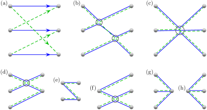
Figure 1: (Color online) The trajectory sets with encounters that contribute to the 3rd correlation function $C(\epsilon,3)$

In this paper we want to show how (4,5,6) can be obtained using the trajectory based methods developed in Refs. Sie, ; Mul1, ; Ric, ; Heu1, . In Sec. II we consider the first term in (4): we show that the prefactor $C(\epsilon,n)$ of the exponential is indeed given by the RMT expression obtained in Ref. Kui, and that this is multiplied by the exponential given in (5). The underlying diagrams considered here are the same as the ones occurring also in the semiclassical calculation of the RMT contribution. In Sec. III we consider the second term in (4) and show how this contribution arises from trajectories that are always correlated. Furthermore we show in Sec. IV that there exist no mixed terms between the first and the second term in (4), that could result - expressed in terms of the considered diagrams - from correlations between trajectories always correlated with each other on the one side and trajectories only correlated with each other during encounters on the other side.

II Influence of the Ehrenfest time on trajectories with encounters

The main idea in this section is to split our diagrams in a different way compared to the semiclassical analysis without Ehrenfest time (referred to as the RMT-treatment) and the analysis of the Ehrenfest-time dependence of the cases $n=1,2,3$ in Ref. Bro, : in the semiclassical calculation one considers an arbitrary number of orbits encountering each other. It turns out in the RMT-treatment to be sufficient to consider only encounters where all orbits are linearizable up to the same point, see for example Fig. 2. When taking into account the Ehrenfest-time dependence this is no longer sufficient as was first shown in Ref. Bro, ; see Fig. 3 for an example of an additional diagram analyzed in this case. The main complication arising in Ref. Bro, is then to treat these encounters. To simplify the calculation we imagine these encounters being built up out of several encounters, each of which consist of two encounter stretches. We have distinguished these 2-encounters by different boxes in Fig. 4. In this way it is much easier to consider encounter diagrams of arbitrary complexity with finite Ehrenfest time, which did not appear in the formalism used in Ref. Bro, .

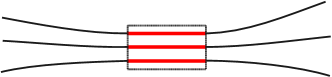
Figure 2: (Color online) A 3-encounter as it can be approximated in the RMT-treatment (c.f. Fig. 1c). The encounter stretches are marked by a box (shown red).

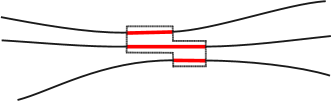
Figure 3: (Color online) A 3-encounter as previously treated with Ehrenfest time Bro . The encounter stretches are marked by a box (shown red).

We first illustrate our procedure by considering three correlated orbits with two 2-encounters as in Fig. 4 and show how the result given in Ref. Bro, can be obtained in this case and then we treat the general case of $n$ orbits with $\left(n-1\right)$ independent or overlapping 2-encounters.

II.1 Explanation of our procedure for $n=3$

In the treatment of the RMT-type contribution (5) we first consider the case in which all the encounters occur inside the system. For $n=3$ we have the two semiclassical diagrams in Fig. 1b,c which include a trajectory set (of three original trajectories and three partners) with two 2-encounters in Fig. 1b and a single 3-encounter in Fig. 1c. By shrinking the link connecting the two encounters in Fig. 1b we can see how we deform them into the diagram in Fig. 1c and we use this idea in our Ehrenfest-time treatment.

II.1.1 Two 2-encounters

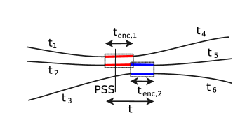
Figure 4: (Color online) A diagram with two 2-encounters as we treat it with Ehrenfest time. The encounter stretches of the two 2-encounters are marked by boxes (shown red and blue). A possible position of the Poincaré surface of section (PSS) is marked by a black vertical line.

For the calculation of contributions resulting from diagrams differing in encounters we first need to review the notation and the important steps of the corresponding calculation in Ref. Mul1, . An encounter of two orbits is characterized by the difference of the stable and unstable coordinates $s_{i}$ and $u_{i}$ measured in a Poincaré surface of section (PSS) put inside the encounter; see Fig. 4. In terms of these coordinates the duration of the encounters is given by $t_{{\rm enc},i}=1/\lambda\ln\left(c^{2}/\left|s_{i}u_{i}\right|\right)$ derived from the condition that the coordinates $s_{i},u_{i}$ are only allowed to grow up to a classical constant $c$ (which is later related to the Ehrenfest time). The weight function measuring the probability to find these encounters is obtained by integrating over all possible positions where the encounter stretches can be placed and dividing by the volume of available phase space (in the corresponding closed system) $\Omega$ and further by the durations of the encounters $t_{{\rm enc},i}$ to avoid overcounting the same set of correlated trajectories. The action difference $\Delta S$ between the orbits is in general given by a quadratic form of the coordinates $s_{i},u_{i}$ determined by where the partner trajectories must pierce the PSS’s to reconnect in the right way to form a closed cycle. For example for a 3-encounter one obtains Mul1 $\Delta S=s_{1}^{\prime}u_{1}^{\prime}+s_{2}^{\prime}u_{2}^{\prime}-s_{1}^{\prime}u_{2}^{\prime}$ where the prime denotes that the coordinates are measured in one PSS from the central trajectory. If we instead measure the coordinates in two different sections, we obtain $\Delta S=s_{1}u_{1}+s_{2}u_{2}-s_{1}u_{2}\exp{(-\lambda\Delta t)}$ where the time $\Delta t$ denotes the time the particle needs to travel between the two sections. This leads in the limit of well separated encounters to $\Delta S\approx s_{1}u_{1}+s_{2}u_{2}$. From this and from Ref. Mul1, we can draw the following conclusions for the form of the action difference in the case of an arbitrary number of (possibly overlapping) 2-encounters: In the case of $k$ well separated 2-encounters we obtain for the action difference $\Delta S\approx\sum_{i=1}^{k}s_{i}u_{i}$. When these encounters overlap the action difference can differ from the last expression by terms exponentially damped with the time difference between the two sections.

In our treatment, the overall contribution $C^{\ref{fig4}}(\epsilon,\tau,3)$ of the two 2-encounters (depicted in more detail in Fig. 4) is obtained by allowing the upper trajectory to possess a minimal length of the first 2-encounter and the lowest one a minimal length of the second 2-encounter. The middle trajectory, which passes through both encounters has a minimal length given by the maximum of the two encounter times as we allow the encounters to overlap. However we do not yet allow one encounter to be subsumed into the other so we also set the time $t$ between the start of the first encounter and the end of the second to be longer than the maximum encounter time. To write down the semiclassical contribution of the diagram in Fig. 4 we sum over the number of possible classical orbits using the open sum rule Ric . Converting the time integrals resulting from this rule to time integrals with respect to link durations, we obtain

$$C^{\ref{fig4}}(\epsilon,\tau,3) = \frac{N^{2}}{\tau_{\mathrm{D}}^{3}}\left(\prod_{i=1}^{6}\int_{0}^{\infty}{\rm d}t_{i}{\rm e}^{-t_{i}\left(1-{\rm i}\epsilon\right)/\tau_{\mathrm{D}}}\right)$$

$$\times\int_{-c}^{c}{\rm d}^{2}s{\rm d}^{2}u\frac{{\rm e}^{{\rm i}\epsilon\left(t_{{\rm enc},1}+t_{{\rm enc},2}\right)/\tau_{\mathrm{D}}}}{\Omega^{2}t_{{\rm enc},1}t_{{\rm enc},2}}$$

$$\times\int_{\max\left\{t_{{\rm enc},1},t_{{\rm enc},2}\right\}}^{\infty}{\rm d}t\,{\rm e}^{\left({\rm i}/\hbar\right)\Delta S}{\rm e}^{-t\left(1-{\rm i}\epsilon\right)/\tau_{\mathrm{D}}},$$

where the superscript refers to Fig. 4. We have summed over the possible channels, and $t_{i}$ with $i=1,\ldots,6$ label the links from the channels to the encounters. In (II.1.1) where ${\rm d}^{2}s={\rm d}s_{1}{\rm d}s_{2}$ and ${\rm d}^{2}u={\rm d}u_{1}{\rm d}u_{2}$, $s_{i}$ and $u_{i}$ with $i=1,2$ are the stable and unstable coordinate differences between the two parts of the trajectories piercing through a PSS placed in the $i$-th encounter. As explained above, the action difference is given by $\Delta S=s_{1}u_{1}+s_{2}u_{2}-s_{1}u_{2}\exp{(-\lambda\Delta t)}$. By expanding the part of the exponential ${\rm e}^{({\rm i}/\hbar)\Delta S}$ containing this $\Delta t$-dependent part into a Taylor series one verifies easily that contributions from higher order terms than the leading (time independent) one are of higher order in $1/\left(\lambda\tau_{D}\right)$ and can be neglected. This reasoning also holds for diagrams with more than two 2-encounters.

In the first line of (II.1.1) we can see that each integral over the links is weighted by its classical probability to remain inside the system for the time $t_{i}$ which decays exponentially with the average dwell time $\tau_{\mathrm{D}}$. We only want to consider trajectory sets where the whole diagram remains inside the system, as if any parts were to hit the lead and escape the diagram would be truncated at that point. With the energy dependence in (7) this gives the factors ${\rm e}^{-t_{i}\left(1-{\rm i}\epsilon\right)/\tau_{\mathrm{D}}}$ in (II.1.1). Inside the encounters however we have trajectory stretches that are so close that the conditional survival probability of secondary traversals is 1 and we need only consider the survival probability of one stretch. If that stretch does not escape then neither will the other. The energy dependence still depends on the total time so that encounter 1 would lead to the factor ${\rm e}^{-t_{{\rm enc},1}\left(1-2{\rm i}\epsilon\right)/\tau_{\mathrm{D}}}$. With the overlap, encounter 2 would then have a more complicated exponential factor, but because the time $t$ (between the two outer ends of the encounter stretches on the middle trajectory shown in Fig. 4) passes through both encounters their survival probability (of both stretches of both encounters) can be expressed as the survival probability of a stretch of duration $t$ as in the last line of (II.1.1). The energy dependence instead also requires the extra traversal of the encounters as given by the exponential factor in the middle line of (II.1.1).

Performing the integrals in the first line of (II.1.1) we have

$$C^{\ref{fig4}}(\epsilon,\tau,3)=\frac{\tau_{\mathrm{D}}T_{\mathrm{H}}^{2}}{(1-{\rm i}\epsilon)^{6}}F^{\ref{fig4}}(\tau),$$ (9)

where we have moved all of the Ehrenfest-time dependent parts into the factor $F^{\ref{fig4}}(\tau)$ with the superscript again referring to Fig. 4,

$$F^{\ref{fig4}}(\tau) = \int_{-c}^{c}{\rm d}^{2}s{\rm d}^{2}u\frac{{\rm e}^{\left({\rm i}/\hbar\right)\Delta S}{\rm e}^{{\rm i}\epsilon\left(t_{{\rm enc},1}+t_{{\rm enc},2}\right)/\tau_{\mathrm{D}}}}{\Omega^{2}t_{{\rm enc},1}t_{{\rm enc},2}}$$ (10)

$$\times\int_{\max\left\{t_{{\rm enc},1},t_{{\rm enc},2}\right\}}^{\infty}{\rm d}t\,{\rm e}^{-t\left(1-{\rm i}\epsilon\right)/\tau_{\mathrm{D}}}.$$

Here we can also see the connection with the previous Ehrenfest-time treatment of such a diagram. When $t>t_{{\rm enc},1}+t_{{\rm enc},2}$ the two encounters separate (the integrals can then be further broken down into products) and this is the case in which the trajectories can be considered to have two independent 2-encounters as in Ref. Bro, . Because we choose a different lower limit however, the contribution above also includes some of the diagrams previously treated as 3-encounters in Ref. Bro, . The reason for our choice becomes clear in the following steps. We first substitute $t^{\prime}=t-\max\left\{t_{{\rm enc},1},t_{{\rm enc},2}\right\}$,

$$F^{\ref{fig4}}(\tau) = \int_{-c}^{c}{\rm d}^{2}s{\rm d}^{2}u\frac{{\rm e}^{\left({\rm i}/\hbar\right)\Delta S}{\rm e}^{{\rm i}\epsilon\left(t_{{\rm enc},1}+t_{{\rm enc},2}\right)/\tau_{\mathrm{D}}}}{\Omega^{2}t_{{\rm enc},1}t_{{\rm enc},2}}$$

$$\times\int_{0}^{\infty}{\rm d}t^{\prime}\,{\rm e}^{-(t^{\prime}+\max\left\{t_{{\rm enc},1},t_{{\rm enc},2}\right\})\left(1-{\rm i}\epsilon\right)/\tau_{\mathrm{D}}},$$

and then substitute $u_{i}=c/\sigma_{i}$, $s_{i}=cx_{i}\sigma_{i}$ and perform the $\sigma_{i}$-integrals using the explicit form of the $t_{{\rm enc},i}=1/\lambda\ln\left(c^{2}/\left|s_{i}u_{i}\right|\right)$ (for details of this calculation, see also Ref. Bro, ). This results in

$$F^{\ref{fig4}}(\tau) = 16\int_{0}^{1}{\rm d}x^{2}\frac{\lambda^{2}c^{4}}{\Omega^{2}}\cos\left(\frac{c^{2}}{\hbar}x_{1}\right)\cos\left(\frac{c^{2}}{\hbar}x_{2}\right)$$ (12)

$$\times\int_{0}^{\infty}{\rm d}t^{\prime}\,{\rm e}^{-\left(t^{\prime}+\max\left\{-\ln x_{1},-\ln x_{2}\right\}/\lambda\right)\left(1-{\rm i}\epsilon\right)/\tau_{\mathrm{D}}}$$

$$\times{\rm e}^{-{\rm i}\epsilon\left(\ln x_{1}+\ln x_{2}\right)/(\lambda\tau_{\mathrm{D}})}.$$

Now we substitute $x_{i}^{\prime}=x_{i}c^{2}/\hbar$ and obtain

$$F^{\ref{fig4}}(\tau) = 16\int_{0}^{\infty}{\rm d}{x^{\prime}}^{2}\frac{\lambda^{2}\hbar^{2}}{\Omega^{2}}\cos\left(x^{\prime}_{1}\right)\cos\left(x^{\prime}_{2}\right)$$ (13)

$$\times\int_{0}^{\infty}{\rm d}t^{\prime}\,{\rm e}^{-\left(t^{\prime}+\max\left\{-\ln x^{\prime}_{1},-\ln x^{\prime}_{2}\right\}/\lambda\right)\left(1-{\rm i}\epsilon\right)/\tau_{\mathrm{D}}}$$

$$\times{\rm e}^{-{\rm i}\epsilon\left(\ln x^{\prime}_{1}+\ln x^{\prime}_{2}\right)/(\lambda\tau_{\mathrm{D}})}{\rm e}^{-\tau\left(1-3{\rm i}\epsilon\right)}.$$

Here we split the resulting expression into an $\hbar$-independent integral (or more exactly trivially dependent on $\hbar$), that exists due to the energy average that is always contained in our calculations, and an Ehrenfest-time or $\hbar$ dependent part with $\tau_{\mathrm{E}}\equiv 1/\lambda\ln\left(c^{2}/\hbar\right)$. This contains the Ehrenfest-time dependence that is expected from (5), so (13) already shows that the diagrams considered here yield the correct Ehrenfest-time dependence.

II.1.2 A 3-encounter

Now we consider the case in which one of the two 2-encounters lies fully inside the other one, which we will refer to as a generalized version of a 3-encounter, as depicted in Fig. 5.

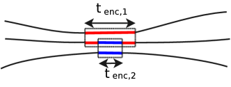
Figure 5: (Color online) One 2-encounter is located fully inside the other, corresponding to our treatment of a generalized version of a 3-encounter. The two 2-encounters are marked by boxes (indicated by different colors).

For the Ehrenfest-time dependent part we have a similar contribution as in (10) with two differences: First $t$ is best defined as the distance between the midpoints of the two different encounter stretches and so it can vary between

$$|t| \leq \frac{1}{2}\left(\max\left\{t_{{\rm enc},1},t_{{\rm enc},2}\right\}-\min\left\{t_{{\rm enc},1},t_{{\rm enc},2}\right\}\right),$$

$$|t| \leq \frac{1}{2}|t_{{\rm enc},1}-t_{{\rm enc},2}|.$$ (14)

Second the survival probability of the encounters is determined by the longest encounter stretch and is independent of $t$. The Ehrenfest-time dependent part can then be written as

$$F^{\ref{fig5}}(\tau) = \int_{-c}^{c}{\rm d}^{2}s{\rm d}^{2}u\frac{{\rm e}^{\left({\rm i}/\hbar\right)\Delta S}{\rm e}^{{\rm i}\epsilon\left(t_{{\rm enc},1}+t_{{\rm enc},2}\right)/\tau_{\mathrm{D}}}}{\Omega^{2}t_{{\rm enc},1}t_{{\rm enc},2}}$$

$$\times\int_{-\frac{1}{2}|t_{{\rm enc},1}-t_{{\rm enc},2}|}^{\frac{1}{2}|t_{{\rm enc},1}-t_{{\rm enc},2}|}{\rm d}t\,{\rm e}^{-(\max\left\{t_{{\rm enc},1},t_{{\rm enc},2}\right\})\left(1-{\rm i}\epsilon\right)/\tau_{\mathrm{D}}}.$$

Performing the $t$ integral and following the same steps as for (12,13), we find

$$F^{\ref{fig5}}(\tau) = 16\int_{0}^{\infty}{\rm d}{x^{\prime}}^{2}\frac{\lambda^{2}\hbar^{2}}{\Omega^{2}}\frac{|\ln x^{\prime}_{1}-\ln x^{\prime}_{2}|}{\lambda}\cos\left(x^{\prime}_{1}\right)$$ (16)

$$\times\cos\left(x^{\prime}_{2}\right){\rm e}^{-\left(\max\left\{-\ln x^{\prime}_{1},-\ln x^{\prime}_{2}\right\}\right)\left(1-{\rm i}\epsilon\right)/(\lambda\tau_{\mathrm{D}})}$$

$$\times{\rm e}^{-{\rm i}\epsilon\left(\ln x^{\prime}_{1}+\ln x^{\prime}_{2}\right)/(\lambda\tau_{\mathrm{D}})}{\rm e}^{-\tau\left(1-3{\rm i}\epsilon\right)}.$$

This part also shows an Ehrenfest-time dependence as expected from (5). Note that when performing the $t$-integral the result in this case is of course proportional to $|t_{{\rm enc},1}-t_{{\rm enc},2}|$ which contains, after the substitution from $x$ to $x^{\prime}$, two times the same terms linear in $\tau_{\mathrm{E}}$ with different signs that thus cancel each other.

II.1.3 Touching the lead

Up to now we have concentrated on encounters inside the system, but apart from these diagrams we also need to consider diagrams where the encounters touch the opening as in Fig. 1d-h. We will, as above, start by considering encounters built up out of two 2-encounters and we focus here on how the calculation of the contribution is changed when encounters move into the lead compared to the treatment of encounters inside the system. As can also be found in more detail in Ref. Bro, when encounters touch the lead one includes in the semiclassical expressions for encounters inside the system an additional time integral running between zero and the corresponding encounter time, which characterizes the duration of the part of the encounter stretch that has not yet been moved into the lead.

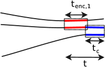
Figure 6: (Color online) The second of two 2-encounters now enters the lead so that only $t_{c}$ of it remains inside the system.

We consider two encounters with durations $t_{{\rm enc},1}$ and $t_{{\rm enc},2}$ with the second encounter touching the opening as in Fig. 1d and drawn in more detail in Fig. 6. As the second encounter enters the lead we now define the time $t$ to be from the start of the first encounter until the lead and introduce the time $t_{c}$ which measures the part of the second encounter that has not yet been moved into the lead. We also separate the Ehrenfest-time relevant contribution $F^{\ref{fig6}}(\tau)$ in this detailed calculation into two cases: in the first case (A); $t_{{\rm enc},2}<t_{{\rm enc},1}$; we have $F_{{\rm A}}^{\ref{fig6}}(\tau)$ with the additional integral over the time $t_{c}$

$$F_{{\rm A}}^{\ref{fig6}}(\tau) = \int_{\begin{subarray}{l}-c\\ t_{{\rm enc},2}<t_{{\rm enc},1}\end{subarray}}^{c}{\rm d}^{2}s{\rm d}^{2}u\frac{{\rm e}^{\left({\rm i}/\hbar\right)\Delta S}{\rm e}^{{\rm i}\epsilon t_{{\rm enc},1}/\tau_{\mathrm{D}}}}{\Omega^{2}t_{{\rm enc},1}t_{{\rm enc},2}}$$

$$\times\int_{0}^{t_{{\rm enc},2}}{\rm d}t_{c}\,{\rm e}^{{\rm i}\epsilon t_{c}/\tau_{\mathrm{D}}}\int_{t_{{\rm enc},1}}^{\infty}{\rm d}t\,{\rm e}^{-t(1-{\rm i}\epsilon)/\tau_{\mathrm{D}}},$$

where the limits on the time integrals derive from the fact that the first encounter is not allowed to touch the lead (this would be included as a 3-encounter) and that the second must. Performing the time integrals this is

$$F_{{\rm A}}^{\ref{fig6}}(\tau) = \int_{\begin{subarray}{l}-c\\ t_{{\rm enc},2}<t_{{\rm enc},1}\end{subarray}}^{c}{\rm d}^{2}s{\rm d}^{2}u\frac{{\rm e}^{\left({\rm i}/\hbar\right)\Delta S}}{\Omega^{2}t_{{\rm enc},1}t_{{\rm enc},2}}\frac{\tau_{\mathrm{D}}^{2}}{{\rm i}\epsilon(1-{\rm i}\epsilon)}$$ (18)

$$\times\left[{\rm e}^{{\rm i}\epsilon t_{{\rm enc},2}/\tau_{\mathrm{D}}}-1\right]{\rm e}^{-t_{{\rm enc},1}(1-2{\rm i}\epsilon)/\tau_{\mathrm{D}}},$$

with the first and second term in the square brackets resulting from the upper and lower limit of the $t_{c}$-integration. In the second case (B); $t_{{\rm enc},2}>t_{{\rm enc},1}$; we obtain

$$F_{{\rm B}}^{\ref{fig6}}(\tau) = \int_{\begin{subarray}{l}-c\\ t_{{\rm enc},2}>t_{{\rm enc},1}\end{subarray}}^{c}{\rm d}^{2}s{\rm d}^{2}u\frac{{\rm e}^{\left({\rm i}/\hbar\right)\Delta S}{\rm e}^{{\rm i}\epsilon t_{{\rm enc},1}/\tau_{\mathrm{D}}}}{\Omega^{2}t_{{\rm enc},1}t_{{\rm enc},2}}$$

$$\times\left[\int_{0}^{t_{{\rm enc},1}}{\rm d}t_{c}\,{\rm e}^{{\rm i}\epsilon t_{c}/\tau_{\mathrm{D}}}\int_{t_{{\rm enc},1}}^{\infty}{\rm d}t\,{\rm e}^{-t(1-{\rm i}\epsilon)/\tau_{\mathrm{D}}}\right.$$

$${}+\left.\int_{t_{{\rm enc},1}}^{t_{{\rm enc},2}}{\rm d}t_{c}\,{\rm e}^{{\rm i}\epsilon t_{c}/\tau_{\mathrm{D}}}\int_{t_{c}}^{\infty}{\rm d}t\,{\rm e}^{-t(1-{\rm i}\epsilon)/\tau_{\mathrm{D}}}\right],$$

where the more complicated limits derive from not allowing the second encounter to move further left than the first. After integrating we have

$$F_{{\rm B}}^{\ref{fig6}}(\tau) = \int_{\begin{subarray}{l}-c\\ t_{{\rm enc},2}>t_{{\rm enc},1}\end{subarray}}^{c}{\rm d}^{2}s{\rm d}^{2}u\frac{{\rm e}^{\left({\rm i}/\hbar\right)\Delta S}}{\Omega^{2}t_{{\rm enc},1}t_{{\rm enc},2}}\frac{\tau_{\mathrm{D}}^{2}}{(1-{\rm i}\epsilon)}$$

$$\times\left[\frac{1}{{\rm i}\epsilon}\left[{\rm e}^{{\rm i}\epsilon t_{{\rm enc},1}/\tau_{\mathrm{D}}}-1\right]{\rm e}^{-t_{{\rm enc},1}(1-2{\rm i}\epsilon)/\tau_{\mathrm{D}}}\right.$$

$${}+\frac{1}{(1-2{\rm i}\epsilon)}{\rm e}^{-t_{{\rm enc},1}(1-3{\rm i}\epsilon)/\tau_{\mathrm{D}}}$$

$${}-\left.\frac{1}{(1-2{\rm i}\epsilon)}{\rm e}^{{\rm i}\epsilon t_{{\rm enc},1}/\tau_{\mathrm{D}}}{\rm e}^{-t_{{\rm enc},2}(1-2{\rm i}\epsilon)/\tau_{\mathrm{D}}}\right].$$

The last line comes from the upper limit of the second $t_{c}$-integral and has the same Ehrenfest-time dependence as before and in line with (5). Likewise the upper $t_{c}$ time limit for case A in (II.1.3) leads to the same dependence and we can conclude that the upper limits of the $t_{c}$-integrations yield contributions similar to when the encounters are inside the system and with the same Ehrenfest-time dependence. The remaining (lower) limits of the time integrations in (II.1.3,II.1.3) give contributions possessing a different Ehrenfest-time dependence which however always yield zero in the semiclassical limit due to the fact that the corresponding terms contain no $t_{{\rm enc},2}$ in the exponentials containing $\tau_{\mathrm{D}}$. Apart from the action difference, the only term depending on $s_{2},u_{2}$ is the $1/t_{{\rm enc},2}$. The resulting expression is rapidly oscillating as a function of the energy Mul1 and thus canceled by the energy average.

We can repeat this procedure for the remaining diagrams in Fig. 1 and see that the contributions are determined by the upper limits of the corresponding $t_{c}$ integrals. For the diagrams with a generalized 3-encounter (Fig. 1g,h) this follows as for the 3-encounter inside the system but for Fig. 1e where the two 2-encounters enter different channels (and possibly different leads) there is an additional subtlety. The two encounters are still allowed to overlap, so that during the time $t$ the stretch now connecting both channels can always be inside encounters but the individual encounters are not allowed to connect leads at both ends. These additional possibilities are considered later, where if both encounters connect to the leads at both ends we actually have a band of correlated trajectories (treated in Sec. III) and if only one does we have a mixed term (treated in Sec. IV). With this organization of the encounters we see that each diagram has the same Ehrenfest-time dependence as when the encounters are inside the system, which is in line with (5).

II.1.4 Intermediate summary

The reasoning so far in this section proves the form of (5) for $n=3$. First of all, we know that the resulting contribution from the diagrams analyzed contains an overall factor ${\rm e}^{-\tau(1-3{\rm i}\epsilon)}$. Secondly, the remaining integrals are independent of $\hbar$ and thus independent of the Ehrenfest time. Thirdly, the diagrams we analyze are the same as the ones analyzed in the RMT-case in the first part of Ref. Kui, . As in the limit $\tau_{\mathrm{E}}\to 0$ we must recover that previous result, this implies that $C(\epsilon,\tau,3)$ in (5) is indeed given by the RMT-expression.

II.1.5 Full contributions

Before proceeding to the general case however, we first want to illustrate how our calculation can be used to obtain, apart from just the Ehrenfest-time dependence, the complete dependence on $\tau_{\mathrm{D}}$ and $\epsilon$.

We therefore start for the two 2-encounters from Fig. 4 from the last expression in (13) and perform first the $t^{\prime}$-integral

$$F^{\ref{fig4}}(\tau) = \frac{16\tau_{\mathrm{D}}}{\left(1-{\rm i}\epsilon\right)}\int_{0}^{\infty}{\rm d}{x^{\prime}}^{2}\frac{\lambda^{2}\hbar^{2}}{\Omega^{2}}\cos\left(x^{\prime}_{1}\right)\cos\left(x^{\prime}_{2}\right)$$ (21)

$$\times{\rm e}^{-\max\left\{-\ln x^{\prime}_{1},-\ln x^{\prime}_{2}\right\}\left(1-2{\rm i}\epsilon\right)/(\lambda\tau_{\mathrm{D}})}$$

$$\times{\rm e}^{\min\left\{-\ln x^{\prime}_{1},-\ln x^{\prime}_{2}\right\}{\rm i}\epsilon/(\lambda\tau_{\mathrm{D}})}{\rm e}^{-\tau\left(1-3{\rm i}\epsilon\right)},$$

where it is simpler to rewrite the result in terms of the maximum and minimum value of $\ln x^{\prime}_{i}$. For calculating the $x^{\prime}_{i}$-integrals we perform partial integrations (integrating each time the $\cos$ functions) and then perform the resulting integrals from zero to infinity

$$F^{\ref{fig4}}(\tau) = -\frac{16{\rm i}\epsilon}{\tau_{\mathrm{D}}}\frac{\left(1-2{\rm i}\epsilon\right)}{\left(1-{\rm i}\epsilon\right)}\int_{0}^{\infty}{\rm d}{x^{\prime}}^{2}\frac{\hbar^{2}}{\Omega^{2}}\frac{\sin\left(x^{\prime}_{1}\right)}{x^{\prime}_{1}}\frac{\sin\left(x^{\prime}_{2}\right)}{x^{\prime}_{2}}$$ (22)

$$\times{\rm e}^{-\max\left\{-\ln x^{\prime}_{1},-\ln x^{\prime}_{2}\right\}\left(1-2{\rm i}\epsilon\right)/(\lambda\tau_{\mathrm{D}})}$$

$$\times{\rm e}^{\min\left\{-\ln x^{\prime}_{1},-\ln x^{\prime}_{2}\right\}{\rm i}\epsilon/(\lambda\tau_{\mathrm{D}})}{\rm e}^{-\tau\left(1-3{\rm i}\epsilon\right)}$$

$$= -\frac{{\rm i}\epsilon}{\tau_{\mathrm{D}}T_{\mathrm{H}}^{2}}\frac{\left(1-2{\rm i}\epsilon\right)}{\left(1-{\rm i}\epsilon\right)}{\rm e}^{-\tau\left(1-3{\rm i}\epsilon\right)}.$$

In the first line the additional terms due the partial integration are either zero or cancel due to the energy average. The final result in the last line of (22) can be also obtained by replacing $\max\left\{-\ln x_{1}^{\prime},-\ln x_{2}^{\prime}\right\}/\lambda=y_{1}$ and $\min\left\{-\ln x_{1}^{\prime},-\ln x_{2}^{\prime}\right\}/\lambda=y_{2}$ and performing the integrals with respect to $y_{i}$ from zero to infinity.

To evaluate the contribution from the generalized 3-encounter in Fig. 5 we again perform two partial integrations in (16) and obtain

$$F^{\ref{fig5}}(\tau) = \frac{16}{\tau_{\mathrm{D}}}\left(1-{\rm i}\epsilon\right)\int_{0}^{\infty}{\rm d}{x^{\prime}}^{2}\frac{\hbar^{2}}{\Omega^{2}}\frac{\sin\left(x^{\prime}_{1}\right)}{x^{\prime}_{1}}\frac{\sin\left(x^{\prime}_{2}\right)}{x^{\prime}_{2}}$$ (23)

$$\times{\rm e}^{-\max\left\{-\ln x^{\prime}_{1},-\ln x^{\prime}_{2}\right\}\left(1-2{\rm i}\epsilon\right)/(\lambda\tau_{\mathrm{D}})}$$

$$\times{\rm e}^{\min\left\{-\ln x^{\prime}_{1},-\ln x^{\prime}_{2}\right\}{\rm i}\epsilon/(\lambda\tau_{\mathrm{D}})}{\rm e}^{-\tau\left(1-3{\rm i}\epsilon\right)}$$

$$= \frac{\left(1-{\rm i}\epsilon\right)}{\tau_{\mathrm{D}}T_{\mathrm{H}}^{2}}{\rm e}^{-\tau\left(1-3{\rm i}\epsilon\right)},$$

where we have also left out the terms from the partial integrations that cancel due to the energy average.

With these results we can now show how they connect to the RMT-type results. For this we need to split our diagrams differently and first we need the result for an ideal 3-encounter as depicted in Fig. 2 whose contribution was calculated Bro to be

$$F^{\ref{fig2}}(\tau)=-\frac{\left(1-3{\rm i}\epsilon\right)}{\tau_{\mathrm{D}}T_{\mathrm{H}}^{2}}{\rm e}^{-\tau\left(1-3{\rm i}\epsilon\right)}.$$ (24)

With the extra factors in (9) it is clear how in the limit $\tau_{\mathrm{E}}=0$ this reduces to the RMT-type result for a 3-encounter as in Ref. Kui, . All the remaining contributions should be collected together as two 2-encounters, and as the ideal 3-encounter is included in our generalized 3-encounter we first subtract (24) from (23)

$$F^{\ref{fig5}}(\tau)-F^{\ref{fig2}}(\tau)=2\frac{\left(1-2{\rm i}\epsilon\right)}{\tau_{\mathrm{D}}T_{\mathrm{H}}^{2}}{\rm e}^{-\tau\left(1-3{\rm i}\epsilon\right)}.$$ (25)

Before we add the result from our separation of two 2-encounters in (22) we remember that in the treatment we enforce that the first encounter is to the left of the second. The result in (25) does not have this restriction so we divide by 2 to ensure compatibility and then add the result in (22) to obtain

$$F^{\ref{fig3}}(\tau)=\frac{1}{\tau_{\mathrm{D}}T_{\mathrm{H}}^{2}}\frac{\left(1-2{\rm i}\epsilon\right)^{2}}{\left(1-{\rm i}\epsilon\right)}{\rm e}^{-\tau\left(1-3{\rm i}\epsilon\right)}.$$ (26)

This then reduces to the RMT-type result for trajectories with two 2-encounters when $\tau_{\mathrm{E}}=0$ as in Ref. Kui, . The agreement of these results with the previous Ehrenfest-time treatmentBro can be seen as the result in (26) including both the result from two independent 2-encounters as well as most of the contribution of the diagram referred to as a 3-encounter in Ref. Bro, . When splitting the contribution in a different way as in Ref. Bro, this also leads to terms in both classes that contain different Ehrenfest-time dependencies that only cancel when summed together.

II.2 All orders

Although up to now we have just reproduced results from Ref. Bro, , the procedure used here has the advantage that it yields a simple algorithm for determining the Ehrenfest-time dependence of the corresponding contributions to $C_{1}(\epsilon,\tau,n)$ at arbitrary order. For our example of $n=3$ we showed how it was possible to split the diagrams into two classes that both showed the Ehrenfest-time dependence as expected from (5). We want now to show how to generalize our way of splitting considered for three trajectories to diagrams containing $n$ trajectories.

II.2.1 Ladder diagrams

We start again with the situation in which all of the encounters are inside the system and by considering a case analogous to Fig. 4, but now involving $n$ instead of three trajectories. We first take a diagram that consists of a ladder of $(n-1)$ 2-encounters so that the central $n-2$ trajectories each contain two encounter stretches while the two outside trajectories only contain one encounter stretch each. This situation is depicted in Fig. 7 and the encounters are thus characterized by $(n-1)$ $s,u$-coordinates.

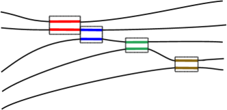
Figure 7: (Color online) A ladder of consecutive 2-encounters. The encounter stretches are marked by boxes (shown in different colors).

In this case we obtain for the Ehrenfest-time relevant contribution $F^{\ref{fig7}}(\tau)$ that the $t$-integral measuring the time difference between the end points of the two encounter stretches on the middle orbit in (10) is replaced by $n-2$ integrals over times $t_{i}$ with the same meaning as $t$; they measure the time difference between the end points of the two (consecutive) encounter stretches on the central trajectories containing two encounter stretches. These times likewise run from the maximum of the corresponding encounter times to infinity. The survival probability is determined by a single (artificial) stretch that runs through all the encounters so that the exponential term describing the $\tau_{\mathrm{D}}$- and $\epsilon$-dependence is now given by

$${\rm e}^{-\sum_{i=1}^{n-2}t_{i}\left(1-{\rm i}\epsilon\right)/\tau_{D}}{\rm e}^{\sum_{i=2}^{n-2}t_{{\rm enc},i}/\tau_{\mathrm{D}}}{\rm e}^{{\rm i}\epsilon\left(t_{{\rm enc},1}+t_{{\rm enc},n-1}\right)/\tau_{\mathrm{D}}},$$ (27)

where $t_{{\rm enc},i}$ are the durations of the $(n-1)$ individual 2-encounters and the middle exponential compensates for the fact that the middle encounters are traversed by two $t_{i}$ and that only one traversal should contribute to the survival probability. Setting $t^{\prime}_{i}=t_{i}-\max\left\{t_{{\rm enc},i},t_{{\rm enc},i+1}\right\}$ and repeating now the steps of (12,13) we find the Ehrenfest-time dependent factor in this case to be

$$F^{\ref{fig7}}(\tau) = \left(\frac{4\lambda\hbar}{\Omega}\right)^{n-1}\prod_{j=1}^{n-1}\int_{0}^{\infty}{\rm d}{x^{\prime}_{j}}\cos\left(x^{\prime}_{j}\right)\prod_{i=1}^{n-2}\int_{0}^{\infty}{\rm d}t^{\prime}_{i}$$ (28)

$$\times{\rm e}^{-\sum_{i=1}^{n-2}\left(t^{\prime}_{i}+\max\left\{-\ln x^{\prime}_{i},-\ln x^{\prime}_{i+1}\right\}/\lambda\right)\left(1-{\rm i}\epsilon\right)/\tau_{\mathrm{D}}}$$

$$\times{\rm e}^{-\sum_{i=2}^{n-2}\ln x^{\prime}_{i}/(\lambda\tau_{\mathrm{D}})}{\rm e}^{-{\rm i}\epsilon\left(\ln x^{\prime}_{1}+\ln x^{\prime}_{n-1}\right)/(\lambda\tau_{\mathrm{D}})}$$

$$\times{\rm e}^{-\tau\left(1-{\rm i}n\epsilon\right)},$$

again confirming the Ehrenfest-time dependence of (5).

II.2.2 Single encounter

Along with the case in which none of the encounters in the ladder can move completely inside another, we can look at the opposite extreme where all the encounter stretches lie inside of the encounter $k$ with the longest duration $t_{{\rm enc},k}=\max_{i}\left\{t_{{\rm enc},i}\right\}$ where $t_{{\rm enc},i}$ are the durations of the $(n-1)$ individual 2-encounters with one of the two orbits containing the stretch of duration $t_{{\rm enc},k}$. This situation is like a generalization of the diagram in Fig. 5 and we similarly now define the times $t_{i}$ to be measured between the centers of encounter $i$ and the encounter $k$ of maximum length (with $i\neq k$). Here the same Ehrenfest-time dependence ${\rm e}^{-\tau\left(1-{\rm i}n\epsilon\right)}$ follows by taking into account that each time $t_{i}$ has a range of variation of size $t_{{\rm enc},k}-t_{{\rm enc},i}$ and that the $\tau_{\mathrm{D}}$- and $\epsilon$-dependent exponential in this case is

$${\rm e}^{-t_{{\rm enc},k}\left(1-{\rm i}\epsilon\right)/\tau_{\mathrm{D}}}{\rm e}^{{\rm i}\epsilon\sum_{i=1}^{n-1}t_{{\rm enc},i}/\tau_{\mathrm{D}}}.$$ (29)

This yields for the Ehrenfest-time dependent factor

$$F^{\ref{fig7}^{\prime}}(\tau) = \left(\frac{4\lambda\hbar}{\Omega}\right)^{n-1}\prod_{j=1}^{n-1}\int_{0}^{\infty}{\rm d}{x^{\prime}_{j}}\cos\left(x^{\prime}_{j}\right)$$ (30)

$$\times{\rm e}^{\left(1-{\rm i}\epsilon\right)\ln x^{\prime}_{k}/(\lambda\tau_{\mathrm{D}})}\left[\prod_{\begin{subarray}{c}i=1\\ i\neq k\end{subarray}}^{n-1}\frac{\left(\ln x^{\prime}_{i}-\ln x^{\prime}_{k}\right)}{\lambda}\right]$$

$$\times{\rm e}^{-{\rm i}\epsilon\sum_{i=1}^{n-1}\ln x^{\prime}_{i}/(\lambda\tau_{\mathrm{D}})}{\rm e}^{-\tau\left(1-{\rm i}n\epsilon\right)},$$

confirming again the Ehrenfest-time dependence predicted by (5).

II.2.3 Mixture

Of course it is additionally possible to have a mixed form between these two extreme cases. This means that some 2-encounters only overlap like in the case of a ladder diagram while the others form ‘single’ encounters; see Fig. 8 for a possible diagram. We then have a ladder of ‘combined’ encounters that themselves can be made up of one or more 2-encounters. The treatment of such diagrams is very similar to the treatments above, and the only slight complication is in defining the appropriate times to extract the Ehrenfest-time dependence.

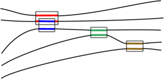
Figure 8: (Color online) One possible example of a mixed case: One encounter is fully contained inside an other, the others form a ladder as considered before.

We recall that the first and last trajectories only pass through one 2-encounter while the central $n-2$ trajectories pass through two. Numbering the central trajectories from $1,\ldots,n-2$, so that trajectory $i$ has encounters $i$ and $i+1$ along it, we divide them into two sets: those whose encounter stretches lie fully inside each other or a connected encounter, as in the case of a single encounter above, that we place in the set $\Omega_{1}$. We place the remaining orbits with two stretches separated as in ladder diagrams in the set $\Omega_{2}$. As mentioned above, we condense the overlapping encounters into combined encounters and record in the set $\Lambda$ the labels of the trajectories that pass through the second stretch in each combined encounter. We also include in this set combined encounters made of a single separated (ladder) 2-encounter. We then use $m(i)$ for $i\in\Lambda$ to record the number of additional consecutive trajectories involved in the same encounter, so that $m(i)=0$ for separated 2-encounters and $m(i)>0$ for larger encounters corresponding to the single encounter case above. If the last combined encounter is a 2-encounter its second stretch is traversed by the last trajectory in the diagram which we number by $n-1$ and include as an element of $\Lambda$. For example, for the diagram in Fig. 8 we would have $\Omega_{1}=\{1\}$, $\Omega_{2}=\{2,3\}$, $\Lambda=\{1,3,4\}$, $m(1)=1$, $m(3)=0$ and $m(4)=0$. For the elements $i\in\Lambda$ we also label by $k_{i}$ the corresponding encounter of maximum length among those from encounter $i$ to encounter $i+m(i)$. To be precise, the two stretches that stay together longest have length $t_{\mathrm{enc},k_{i}}$ while the other encounter times are defined by how long the remaining stretches remain close to one of the two longest.

For the trajectories passing through two separated condensed encounters $i\in\Omega_{2}$ we define the times $t_{i}$ to include the whole of the leftmost and rightmost condensed encounters, i.e. to include the encounters $k_{\bar{i}}$ and $k_{i+1}$, where $\bar{i}$ is the largest element in $\Lambda$ that is $\leq i$. In this case the $\tau_{\mathrm{D}}$- and $\epsilon$-dependent exponential can be written as

$${\rm e}^{-\sum_{i\in\Omega_{2}}t_{i}\left(1-{\rm i}\epsilon\right)/\tau_{\mathrm{D}}}{\rm e}^{\sum_{i\in\bar{\Lambda}}t_{{\rm enc},k_{i}}\left(1-{\rm i}\epsilon\right)/\tau_{\mathrm{D}}}$$

$$\times{\rm e}^{-t_{{\rm enc},k_{1}}\left(1-{\rm i}\epsilon\right)/\tau_{\mathrm{D}}}{\rm e}^{{\rm i}\epsilon\sum_{i=1}^{n-1}t_{{\rm enc},i}/\tau_{\mathrm{D}}},$$ (31)

where $\bar{\Lambda}$ is $\Lambda$ with its largest element removed so that the second term accounts for the overlap between the $t_{i}$’s and the third term for the fact that there is also no overlap at the start of the first such stretch. This equation incorporates both (27) and (29). If we introduce the notation $M[i,j]\equiv\max\left\{t_{{\rm enc},i},t_{{\rm enc},j}\right\}$, we can then define the times $t^{\prime}_{i}=t_{i}-M[k_{\bar{i}},k_{i+1}]$ as before (28). Making the substitutions as done previously yields for the Ehrenfest-time dependent factor

$$F^{\ref{fig7a}}(\tau) = \left(\frac{4\lambda\hbar}{\Omega}\right)^{n-1}\prod_{j=1}^{n-1}\int_{0}^{\infty}{\rm d}{x^{\prime}_{j}}\cos\left(x^{\prime}_{j}\right)\prod_{i\in\Omega_{2}}\int_{0}^{\infty}{\rm d}t_{i}^{\prime}$$ (32)

$$\times\prod_{i\in(\Omega_{1}\cap\Lambda)}\left[\prod_{\begin{subarray}{c}j=i\\ j\neq k_{i}\end{subarray}}^{i+m(i)}\frac{\left(\ln x^{\prime}_{j}-\ln x^{\prime}_{k_{i}}\right)}{\lambda}\right]$$

$${\rm e}^{-\sum_{i\in\Omega_{2}}\left(t^{\prime}_{i}+\hat{M}[k_{\bar{i}},k_{i+1}]/\lambda\right)\left(1-{\rm i}\epsilon\right)/\tau_{\mathrm{D}}}$$

$$\times{\rm e}^{-\sum_{i\in\bar{\Lambda}}\ln x^{\prime}_{k[i]}\left(1-{\rm i}\epsilon\right)/(\lambda\tau_{\mathrm{D}})}{\rm e}^{\ln x^{\prime}_{k[1]}\left(1-{\rm i}\epsilon\right)/(\lambda\tau_{\mathrm{D}})}$$

$$\times{\rm e}^{-{\rm i}\epsilon\sum_{i=1}^{n-1}\ln x^{\prime}_{i}/(\lambda\tau_{\mathrm{D}})}{\rm e}^{-\tau\left(1-{\rm i}n\epsilon\right)},$$

with $\hat{M}[i,j]=\max\left\{-\ln x^{\prime}_{i},-\ln x^{\prime}_{j}\right\}$. As $\Omega_{2}$ and $\bar{\Lambda}$ must have the same number of elements, this again shows the predicted Ehrenfest-time dependence.

II.2.4 General encounters

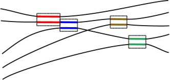
Figure 9: (Color online) A general diagram containing also orbits with more than two stretches. The encounters are marked by boxes (shown in different colors).

Up to now we restricted our discussion to diagrams in which each trajectory is involved in one or two encounters. This is however not yet the most general case where the only restriction is that each trajectory contains at least one encounter stretch, so that some trajectories can also contain more than two encounter stretches. Note that the situation where two trajectories interact (pass through the same 2-encounter block) more than once cannot occur at leading order in inverse channel number. An example of a diagram that is possible is depicted in Fig. 9. In the most general case we define the times $t_{i}$ slightly differently: first we separate the $k\geq 2$ trajectories that have one encounter stretch from the remaining $n-k$ that have more than one. Then we number our encounters accordingly, first those along the trajectories with one encounter stretch with duration $t_{{\rm enc},i}$, $i=1,\ldots,k$ then the remaining encounters with duration $t_{{\rm enc},i}$, $i=k+1,\ldots,n-1$. For the $n-k$ trajectories with two or more encounter stretches we now define $t_{i}$, $i=1,\ldots,n-k$, to be the time difference between the outer edges of the outermost encounters along those trajectories.

For any trajectories with more than two encounter stretches we will need additional time differences to fully fix the positions of the encounters. Because we defined the times $t_{i}$ to go through the outmost encounters, importantly the exponential factor with the survival probability and the energy dependence does not depend on these additional time differences and is given by

$${\rm e}^{-\sum_{i=1}^{n-k}t_{i}\left(1-{\rm i}\epsilon\right)/\tau_{\mathrm{D}}}{\rm e}^{\sum_{i=k+1}^{n-1}t_{{\rm enc},i}/\tau_{\mathrm{D}}}{\rm e}^{{\rm i}\epsilon\sum_{i=1}^{k}t_{{\rm enc},i}/\tau_{\mathrm{D}}}$$ (33)

where the middle term ensures that the survival probability only includes one copy of each encounter and the energy dependence involves all traversals of all the encounters.

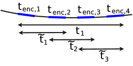
Figure 10: (Color online) Definition of the times $\tilde{t}_{i}$ in the case of more than two encounter stretches on one orbit. The encounter stretches are shown thicker (blue).

For the remaining times we notice that, starting with the ladder system with 2 trajectories containing one encounter stretch and $n-2$ trajectories containing two stretches, every time we increase the number of trajectories with one encounter stretch we simultaneously increase the number with more than two. Therefore there are $k-2$ additional time differences needed to fix the positions of the central encounters along trajectories with more than two and we define times $\tilde{t}_{i}$ for $i=1,\ldots,k-2$ from the left hand side of one encounter stretch to the right hand side of the next encounter stretch following on the right on those trajectories, see also Fig. 10. As the encounters are ordered, they are not (yet) allowed to be subsumed by each other or pushed past the outside encounters. The ranges of the times $\tilde{t}_{i}$ are then fixed by these restrictions. Using again $M[i,j]$ defined after (II.2.3) in the following to make the notation more compact, we obtain for a trajectory containing $m$ encounter stretches of durations $t_{{\rm enc},i}$, $i=1,\ldots,m$, as illustrated in Fig. 10, the integrals

$$\int_{M(1,2)}^{t_{i}}{\rm d}\tilde{t}_{1}\ldots\int_{M[m-2,m-1]}^{t_{i}-\sum_{o=1}^{m-3}\left(\tilde{t}_{o}-M[o,o+1]\right)}{\rm d}\tilde{t}_{m-2}$$

$$= \int_{0}^{t_{i}-M[1,2]}{\rm d}\tilde{t}_{1}^{\prime}\ldots\int_{0}^{t_{i}-\sum_{o=1}^{m-3}\tilde{t}_{o}^{\prime}-M[m-2,m-1]}{\rm d}\tilde{t}_{m-2}^{\prime}.$$

In the second line we substituted $\tilde{t}_{j}^{\prime}=\tilde{t}_{j}-M[j,j+1]$. The time differences $t_{i}$, which are more important for the Ehrenfest-time dependence, must instead just be longer than the maximal length of the encounter stretches lying on the considered trajectory. In general the numbering of the encounters and time differences can be more complicated than in Fig. 10 so we define $l(i)$ to be a list of length $m(i)$ of the encounters enclosed by the time $t_{i}$ (including the outer encounters) and $L(i)$ a list of the corresponding $m(i)-1$ times $\tilde{t}$ between the ends of those encounters. Now we can make the substitution $t^{\prime}_{i}=t_{i}-\max_{j\in l(i)}\left\{t_{{\rm enc},j}\right\}$. After this substitution we recognize that (LABEL:eq32) has become independent of $\hbar$ or the Ehrenfest time. Following then the steps in (12,13) we obtain

$$F^{\ref{fig8}}(\tau) = \left(\frac{4\lambda\hbar}{\Omega}\right)^{n-1}\prod_{j=1}^{n-1}\int_{0}^{\infty}{\rm d}{x^{\prime}_{j}}\cos\left(x^{\prime}_{j}\right)\prod_{i=1}^{n-k}\int_{0}^{\infty}{\rm d}t^{\prime}_{i}$$

$$\times\int_{0}^{t_{i}^{\prime}-\left(\ln x^{\prime}_{\max,i}+\hat{M}[l_{1},l_{2}]\right)/\lambda}{\rm d}\tilde{t}_{L_{1}}^{\prime}\ldots$$

$$\times\int_{0}^{t_{i}^{\prime}-\sum_{o=1}^{m-3}\tilde{t}_{L_{o}}^{\prime}-\left(\ln x^{\prime}_{\max,i}+\hat{M}[l_{m-2},l_{m-1}]\right)/\lambda}{\rm d}\tilde{t}_{L_{m-2}}^{\prime}$$

$$\times{\rm e}^{-\sum_{i=1}^{n-k}\left(t^{\prime}_{i}-\ln x^{\prime}_{\max,i}/\lambda\right)\left(1-{\rm i}\epsilon\right)/\tau_{\mathrm{D}}}$$

$$\times{\rm e}^{-\sum_{i=k+1}^{n-1}\ln x^{\prime}_{i}/(\lambda\tau_{\mathrm{D}})}{\rm e}^{-{\rm i}\epsilon\sum_{i=1}^{k}\ln x^{\prime}_{i}/(\lambda\tau_{\mathrm{D}})}$$ (35)

$$\times{\rm e}^{-\tau\left(1-{\rm i}n\epsilon\right)},$$

with $-\ln x^{\prime}_{\max,i}=\max_{j\in l(i)}\left\{-\ln x^{\prime}_{j}\right\}$ linked to the duration of the longest encounter stretch contained within $t_{i}$. We have also used $\hat{M}[i,j]$ defined after (32) and dropped the explicit $i$ dependence of $l,L$ and $m$ above. Again we obtain the Ehrenfest-time dependence predicted by (5).

As in the case of the ladder diagram above, we can also have the possibility of some encounter stretches being contained in larger encounter stretches and some separated from those larger encounters, see Fig. 11

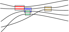
Figure 11: (Color online) An encounter diagram containing also orbits with more than two stretches. In contrast to Fig. 9 encounter stretches here are allowed to be contained fully inside others. The encounters are marked by boxes (shown in different colors).

for an example of a possible diagram. This just implies that some of the $t_{i}$ integrals have to be treated as was done in the case of the configuration shown in Fig. 5, and the Ehrenfest-time dependence predicted by (5) also follows in this case.

II.2.5 Touching the lead

When the encounters are allowed to enter the lead we again have to consider times representing how far each encounter has moved into the lead (actually how much of the encounter remains inside the system). As for the case treated in detail for $n=3$ it is only the upper limit (namely the full encounter time) of these time integrals that have the necessary encounter time dependence to contribute in the semiclassical limit. The reasoning for $n=3$ can then be carried over directly to the more general cases as the upper limits of these integrations yield contributions that are (up to constant factors) the same as the ones obtained when the encounters are inside the system. We thus obtain the same Ehrenfest-time dependence from encounters moved into the leads.

II.3 Summary

The separate diagrams considered in the RMT-type semiclassical treatment Kui can be created from the original collapse of trajectories onto each other and by sliding the individual encounters together or into the leads. The Ehrenfest-time treatment however suggests treating all of these possibilities instead as part of continuous families. What we have shown above in this section is that, if we partition this family in a particular way, for any partition we can find a suitable set of coordinates that allows us to transform the semiclassical contribution so that we can extract the overall Ehrenfest-time dependence. Though the exact details of this transformation depend on the structures of the partition, the algorithmic routines described above all lead to the same Ehrenfest-time dependence. Each partition and hence family then has the factor ${\rm e}^{-\tau\left(1-{\rm i}n\epsilon\right)}$ and no other Ehrenfest-time or $\hbar$ dependence. As we know that we must recover the RMT-type result $C(\epsilon,n)$ in (5) when $\tau_{\mathrm{E}}=0$ (since we treat the same diagrams) with no further Ehrenfest-time dependence, we then obtain the full result in (5) and hence provide a semiclassical justification of the effective RMT ansatz.

III Trajectories always correlated

Figure 12: (Color online) Band of $n=3$ correlated trajectories. The length of the orbits is marked by a box; the duration of the encounter $t_{\rm enc}=1/\lambda\ln\left(c^{2}/{\max}_{i}\left|s_{i}\right|{\max}_{j}\left|u_{j}\right|\right)$ is marked by a dotted box.

In this section we determine the so called classical contribution in (6). To obtain this contribution $C_{2}(\epsilon,\tau,n)$ semiclassically we consider a band of $n$ trajectories that are correlated (inside the same encounter) for their entire duration between entering and leaving the system as in Fig. 12. This implies that all the trajectories have the same length $t$ and that the maximum of the differences $s_{i},u_{i}$ between their stable and unstable coordinates lies below the constant $c$ (related to the Ehrenfest time). For the case $n=2$ this configuration was first considered in Ref. Whi, and then extended to $n=3$ in Ref. Bro, . For our calculation we follow Ref. Bro, and place a PSS at a distance $t_{1}$ from the left end of the trajectories while the remaining time on the right of the section is denoted by $t_{2}=t-t_{1}$. The semiclassical contribution $C_{2}(\epsilon,\tau,n)$ can be written as

$$C_{2}(\epsilon,\tau,n) = \frac{1}{\tau_{\mathrm{D}}}\int_{0}^{\infty}{\rm d}t_{1}\int_{0}^{\infty}{\rm d}t_{2}\frac{{\rm e}^{-t\left(1-{\rm i}n\epsilon\right)/\tau_{\mathrm{D}}}}{(2\pi\hbar)^{n-1}\left(t_{1}+t_{2}\right)}$$

$$\times\int_{|s_{i}|\leq c{\rm e}^{-\lambda t_{1}}}{\rm d}s^{n-1}\int_{|u_{i}|\leq c{\rm e}^{-\lambda t_{2}}}{\rm d}u^{n-1}{\rm e}^{\left({\rm i}/\hbar\right)\Delta S},$$

where we only include one traversal of the band in the survival probability and the restrictions on the $s$ and $u$ integrals ensure that the band always remains together under the exponential divergence of the trajectories due to the chaotic dynamics. Performing an integral over $t_{1}-t_{2}$ and the $u_{i}$ integrals gives

$$C_{2}(\epsilon,\tau,n) = \frac{4^{n-1}}{\tau_{\mathrm{D}}}\int_{0}^{\infty}{\rm d}t\,\frac{{\rm e}^{-t\left(1-{\rm i}n\epsilon\right)/\tau_{\mathrm{D}}}}{(2\pi\hbar)^{n-1}}$$

$$\times\int_{0}^{{\rm e}^{-\lambda t}}{\rm d}x^{n-1}\prod_{i=1}^{n-1}\frac{\hbar}{x_{i}}\sin\left(\frac{c^{2}x_{i}}{\hbar}\right),$$

where $x_{i}={\rm e}^{-\lambda t_{2}}s_{i}/c$. Using that in the semiclassical limit

$$\int_{0}^{{\rm e}^{-\lambda t}}{\rm d}x\frac{\hbar}{x}\sin\left(\frac{c^{2}x}{\hbar}\right)=\frac{\pi\hbar}{2}\Theta\left(\tau_{\mathrm{E}}-t\right),$$ (38)

with the Heaviside theta function $\Theta(x)$, we finally obtain

$$C_{2}(\epsilon,\tau,n)=\frac{1-{\rm e}^{-\tau(1-{\rm i}n\epsilon)}}{1-{\rm i}n\epsilon},$$ (39)

proving the Ehrenfest-time dependence of the $C_{2}(\epsilon,\tau,n)$ in (6).

IV Mixed Terms

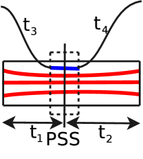
Figure 13: (Color online) An example of a band of three trajectories that possesses an encounter with another trajectory. The band is marked by a thicker box (red stretches), the encounter of the other trajectory with the band by a dotted box (blue stretch) and the links by thin (black) lines. The link durations are denoted by $t_{3}$ and $t_{4}$, and the durations of the band before and after the PSS by $t_{1}$ and $t_{2}$.

Finally we want to consider possible correlations between trajectory structures giving the RMT-type contribution and those giving the classical part, i.e. contributions from correlations between bands of trajectories (that are always correlated with each other) and trajectories that are only correlated with each other during encounters. In particular we want to show that diagrams that have a correlated band that has any encounter with other trajectory structures (with encounters) give no contribution in the semiclassical limit. This, once generalized, then excludes the existence of mixed terms in (4) so that (4) is complete. First we consider the case in which $n-1$ of the trajectories form a correlated band with the remaining trajectory meeting the band in an encounter inside the system as depicted in Fig. 13. This contribution $C^{\ref{fig11}}(\epsilon,\tau,n)$ to the correlation function $C(\epsilon,\tau,n)$ can be written by treating the correlated band as before and introducing the times $t_{3}$ and $t_{4}$ to represent the durations of the parts of the trajectory that encounter the band on the left and on the right of the PSS. It reads

$$C^{\ref{fig11}}(\epsilon,\tau,n) = \frac{1}{\tau_{\mathrm{D}}^{3}}\int_{0}^{\infty}\prod_{i=1}^{4}{\rm d}t_{i}\frac{{\rm e}^{-\sum_{i=1}^{4}t_{i}\left(1-{\rm i}\epsilon\right)/\tau_{\mathrm{D}}}}{(2\pi\hbar)^{n-1}}\hskip 20.00003pt$$ (40)

$$\times\prod_{i=1}^{n-2}\left[\int_{|s_{i}|\leq c{\rm e}^{-\lambda t_{1}}}{\rm d}s^{n-2}\int_{|u_{i}|\leq c{\rm e}^{-\lambda t_{2}}}{\rm d}u^{n-2}\right]$$

$$\times\int_{c{\rm e}^{-\lambda t_{1}}<|s|\leq c}{\rm d}s\int_{c{\rm e}^{-\lambda t_{2}}<|u|\leq c}{\rm d}u$$

$$\times\frac{{\rm e}^{\left({\rm i}/\hbar\right)\Delta S}{\rm e}^{{\rm i}\epsilon\left(t_{\rm enc}+(n-2)(t_{1}+t_{2})\right)/\tau_{\mathrm{D}}}}{\left(t_{1}+t_{2}\right)},$$

where $t_{\rm enc}$ is the time during which the remaining trajectory encounters the band. In this case no overcounting factor $1/t_{\rm enc}$ occurs as the limits of the $s,u$-integrals in the third line are chosen such that the time integral accounting for all possible positions of the single encounter stretch with respect to the band cancels this factor. Choosing different limits for the $s,u$-integrals we could replace the current overcounting factor of $1/\left(t_{1}+t_{2}\right)$ in (40) again by the usual $1/t_{\rm enc}$ as in Sec. II.

The integrals over the $(n-2)$ $s,u$-coordinates within the band are performed in the same manner as in the last section in (38) and lead to the same Heaviside function $\Theta(\tau_{\mathrm{E}}-t)$. For the integrals in the third line in (40) over the differences $s,u$ between the coordinates of a band trajectory and the trajectory encountering it we obtain

$$\int_{c{\rm e}^{-\lambda t_{1}}<|s|\leq c}{\rm d}s\int_{c{\rm e}^{-\lambda t_{2}}<|u|\leq c}{\rm d}u\>{\rm e}^{\left({\rm i}/\hbar\right)su}{\rm e}^{{\rm i}\epsilon t_{\rm enc}/\tau_{\mathrm{D}}}$$ (41)

$$\approx \int_{{\rm e}^{-\lambda t}}^{1}{\rm d}x\frac{4\hbar}{x}\sin\left(\frac{c^{2}x}{\hbar}\right){\rm e}^{{\rm i}\epsilon\tau}$$

$$= \int_{{\rm e}^{-\lambda\left(t-\tau_{\mathrm{E}}\right)}}^{{\rm e}^{\lambda\tau_{\mathrm{E}}}}{\rm d}x^{\prime}\frac{4\hbar}{x}\sin x^{\prime}{\rm e}^{{\rm i}\epsilon\tau}$$

$$= {2\pi\hbar}\Theta\left(t-\tau_{\mathrm{E}}\right){\rm e}^{{\rm i}\epsilon\tau},$$

with $x={\rm e}^{-\lambda t_{2}}s/c$. This Heaviside function is opposite to the one from the band, so that the total contribution vanishes due to the opposing restrictions of the theta functions. Note that when evaluating the Ehrenfest-time dependence of the RMT contributions in Sec. II we chose a different way for performing the integrals. In Sec. II we performed restricted time integrals first and unrestricted $x^{\prime}$ integrals afterwards. The different order of calculating these integrals leads to the theta functions which make it clear that mixed terms like in Fig. 13 vanish; this is why we use this ordering here. If we move more trajectories from the band (composed of at least two trajectories) to the trajectory structure with encounters we still obtain these opposing Heaviside functions and hence no contribution.

A similar reasoning can be applied if the encounter of a trajectory (or part of a trajectory structure) with a band does not happen inside the system but enters the lead at the beginning or the end. In this case we obtain an additional time integral with respect to the time of the encounter that remains inside the system but, as the $s,u$-integrals still yield the same Heaviside functions, this contribution also vanishes. Note that if we move both ends of the encounter into the leads then the encountering trajectory can be considered as part of the band and treated as above or in Sec. III.

The reasoning in this section applies to an arbitrary number of bands of correlated trajectories connected by trajectories that are only correlated in encounters. Therefore all such mixed terms vanish.

V Implications for transport and scattering

V.1 Moments of transmission

Up to now we have concentrated on energy dependent correlation functions involving the whole scattering matrix. Because we use the same semiclassical diagrams our result can be applied directly to dc-transport properties of chaotic systems such as the moments of the transmission or reflection eigenvalues. Assuming the system has two scattering leads and taking just the transmission subblock $t$ of the scattering matrix connecting the $N_{1}$ channels in lead 1 to the $N_{2}$ channels in lead 2 (without an energy difference) the moments of the transmission eigenvalues can be written as

$$M(\tau,n)=\frac{1}{N}{\rm Tr}\left[tt^{\dagger}\right]^{n},$$ (42)

where $N=N_{1}+N_{2}$ is the total number of channels. Within the Landauer-BüttikerLan approach to quantum transport the moments carry information about statistical properties of the transmission in the phase coherent regime, the counting statisticsNaz . For example the first moment characterizes the average conductance $G\propto M(\tau,1)$ and the second one the power of the shot noise $P\propto M(\tau,1)-M(\tau,2)$. Using the semiclassical results from this paper we can simply write

$$M(\tau,n)=M(n){\rm e}^{-\tau}+\frac{N_{1}N_{2}}{N^{2}}\left(1-{\rm e}^{-\tau}\right),$$ (43)

where we have included the probability $N_{1}/N$ of starting in lead 1 in the moments. Equation (43) can be generalized to ac-transport considered in Ref. Petit, by including in the latter equation the $\epsilon$-dependent factors given in (5,6). The result in (43) again splits into two parts with the first involving the semiclassical moments $M(n)$ calculated in Ref. Ber, , which in turn lead to the random matrix probability distribution bb96 ; novaes07 .

The second term in (43) leads to the classical Bernoulli distribution where the transmission amplitude $T$ is 1 with probability $N_{2}/N$ and 0 otherwise (i.e. $N_{1}/N$). The Ehrenfest time then provides a smooth interpolation between these two distributions giving a weight ${\rm e}^{-\tau}$ to the RMT one and the remaining weight $(1-{\rm e}^{-\tau})$ to the classical one. A similar formula and result follows for the moments and probability distribution of the reflection eigenvalues whose zero Ehrenfest time contributions can be simply derived from the treatment in Ref. Ber, .

V.2 Moments of delay times

Taking the full correlation functions $C(\epsilon,\tau,n)$ it is possible to obtain not only the Ehrenfest-time dependence of the density of states of chaotic Andreev systems, covered in detail in Ref. Kui, , but also the moments and distribution of the Wigner delay times. We start with the Wigner-Smith matrix Wig

$$Q=\frac{\hbar}{\rm i}S^{\dagger}(E)\frac{{\rm d}S(E)}{{\rm d}E},$$ (44)

which can be shown to be Hermitian by using the unitarity of the scattering matrix. Because of this unitarity $Q$ can also be written as

$$Q=\frac{\tau_{\mathrm{D}}}{{\rm i}}\frac{{\rm d}}{{\rm d}\epsilon}\left[S^{\dagger}\left(-\frac{\epsilon\hbar}{2\tau_{\mathrm{D}}}\right)S\left(+\frac{\epsilon\hbar}{2\tau_{\mathrm{D}}}\right)\right]\Big{|}_{\epsilon=0},$$ (45)

where the scattering matrix energy differences are measured with respect to the energy $E$. The delay times are simply the eigenvalues of $Q$ so their moments are

$$m(\tau,n)=\frac{1}{N}{\rm Tr}\left[Q\right]^{n}.$$ (46)

Using the relation

$$\frac{1}{n!}\frac{{\rm d}^{n}}{{\rm d}\epsilon^{n}}\left[f(\epsilon)-f(0)\right]^{n}\Big{|}_{\epsilon=0}=\left[f^{\prime}(0)\right]^{n},$$ (47)

the moments of the delay times are Ber2

$$m(\tau,n) = \frac{\tau_{\mathrm{D}}^{n}}{{\rm i}^{n}n!N}\frac{{\rm d}^{n}}{{\rm d}\epsilon^{n}}{\rm Tr}$$

$$\left[S^{\dagger}\left(-\frac{\epsilon\hbar}{2\tau_{\mathrm{D}}}\right)S\left(+\frac{\epsilon\hbar}{2\tau_{\mathrm{D}}}\right)-I\right]^{n}\Big{|}_{\epsilon=0}.$$

Expanding (V.2), the moments can be expressed as

$$m(\tau,n)=\frac{\tau_{\mathrm{D}}^{n}}{{\rm i}^{n}n!}\frac{{\rm d}^{n}}{{\rm d}\epsilon^{n}}\sum_{k=1}^{n}\left(-1\right)^{n-k}\left(\begin{array}[]{c}n\\ k\end{array}\right)C(\epsilon,\tau,k)\Big{|}_{\epsilon=0},$$ (49)

in terms of the correlation functions calculated before. As this is additive we can look at the two parts of the Ehrenfest-time dependent results in (4) separately.

For the first part of the $C_{1}(\epsilon,\tau,k)$ however, it is possible to put our Ehrenfest dependence into the framework of Ref. Ber2, where the moments and the probability distribution $\rho(\tau_{\mathrm{W}})$ of the Wigner delay times $\tau_{\mathrm{W}}$ were calculated (without the Ehrenfest time). We can actually obtain the result in a simple way. Using (47) again we can see that since

$$Q-\tau_{\mathrm{E}}I=\frac{\tau_{\mathrm{D}}}{{\rm i}}\frac{{\rm d}}{{\rm d}\epsilon}\left[S^{\dagger}\left(-\frac{\epsilon\hbar}{2\tau_{\mathrm{D}}}\right)S\left(+\frac{\epsilon\hbar}{2\tau_{\mathrm{D}}}\right){\rm e}^{-{\rm i}\epsilon\tau}\right]\Big{|}_{\epsilon=0},$$ (50)

we have

$$\frac{1}{N}{\rm Tr}\left[Q-\tau_{\mathrm{E}}I\right]^{n} = \frac{\tau_{\mathrm{D}}^{n}}{{\rm i}^{n}n!}\frac{{\rm d}^{n}}{{\rm d}\epsilon^{n}}\sum_{k=1}^{n}$$ (54)

$$\left(-1\right)^{n-k}\left(\begin{array}[]{c}n\\ k\end{array}\right)C(\epsilon,\tau,k){\rm e}^{-{\rm i}k\epsilon\tau}\Big{|}_{\epsilon=0}.$$

Plugging in our result for $C_{1}(\epsilon,\tau,k)$ from (5) the energy dependent exponentials cancel so, apart from the damping factor ${\rm e}^{-\tau}$, we just have the moments without any Ehrenfest-time dependence, leading Ber2 to the RMT result Bro99 . Of course on the left hand side of (54) we have a simple translation by the Ehrenfest time, meaning that the translated probability distribution is the same as the RMT-one (damped). For the full Ehrenfest-time dependent distribution we simply translate back again and have

$$\rho_{1}(\tau_{\mathrm{W}}) = \frac{\sqrt{\left(\tau_{+}-\tau_{\mathrm{W}}\right)\left(\tau_{\mathrm{W}}-\tau_{-}\right)}}{2\pi(\tau_{\mathrm{W}}-\tau_{\mathrm{E}})^{2}}{\rm e}^{-\tau},\quad\tau_{-}<\tau_{\mathrm{W}}<\tau_{+}$$

$$\tau_{\pm} = (3\pm\sqrt{8})\tau_{\mathrm{D}}+\tau_{\mathrm{E}}.$$ (55)

For the second ‘classical’ contribution in (4) we first take the simplest part of the contribution

$$C_{2}^{(1)}(\epsilon,\tau,k)=\frac{1}{1-{\rm i}k\epsilon},$$ (56)

and substitute into (49) obtaining

$$m_{2}^{(1)}(\tau,n)=\tau_{\mathrm{D}}^{n}\sum_{k=1}^{n}\left(-1\right)^{n-k}\left(\begin{array}[]{c}n\\ k\end{array}\right)k^{n}=\tau_{\mathrm{D}}^{n}n!$$ (57)

These moments clearly come from an exponential distribution, so that in the limit $\tau\to\infty$ we recover, for the probability distribution $\rho_{2}^{(1)}(\tau_{\mathrm{W}})$, the classical exponential decay of trajectories inside the system

$$\rho_{2}^{(1)}(\tau_{\mathrm{W}})=\frac{1}{\tau_{\mathrm{D}}}{\rm e}^{-\tau_{\mathrm{W}}/\tau_{\mathrm{D}}},\quad\tau_{\mathrm{W}}>0.$$ (58)

For the remaining contribution of the second part $\rho_{2}^{(2)}(\tau_{\mathrm{W}})$, we have the damping factor ${\rm e}^{-\tau}$, and the energy dependent phase again just leads to a shift in the exponential distribution so this contribution starts at $\tau_{\mathrm{E}}$, thus yielding

$$\rho_{2}^{(2)}(\tau_{\mathrm{W}})=-\frac{1}{\tau_{\mathrm{D}}}{\rm e}^{-\tau_{\mathrm{W}}/\tau_{\mathrm{D}}},\quad\tau_{\mathrm{W}}>\tau_{\mathrm{E}}.$$ (59)

The minus sign however means we truncate the previous exponential at $\tau_{\mathrm{E}}$, so the total second contribution to the probability distribution is

$$\rho_{2}(\tau_{\mathrm{W}})=\frac{1}{\tau_{\mathrm{D}}}{\rm e}^{-\tau_{\mathrm{W}}/\tau_{\mathrm{D}}},\quad 0<\tau_{\mathrm{W}}<\tau_{\mathrm{E}},$$ (60)

and 0 elsewhere. Since this contribution to the delay time probability distribution is considered to be made up of the two distributions $\rho_{1}^{(1)}(\tau_{\mathrm{W}})$ and $\rho_{1}^{(2)}(\tau_{\mathrm{W}})$ and as the shifted and damped one $\rho_{1}^{(2)}(\tau_{\mathrm{W}})$ has the same mean ($\tau_{\mathrm{D}}+\tau_{\mathrm{E}}$) and weight as the shifted and damped RMT distribution $\rho_{1}(\tau_{\mathrm{W}})$ but a minus sign, it is clear that the average time delay stays at $\tau_{\mathrm{D}}$ (i.e. from the untruncated exponential distribution) and is unaffected by the Ehrenfest time. In fact this is an example of the general relation Lyu , derived from the unitarity of the scattering matrix, in which the mean time delay depends just on the average spacing of the resonant levels of the scattering system and the number of scattering channels, i.e. it should have no Ehrenfest time or other dependence.

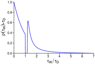
Figure 14: (Color online) The probability density of the Wigner delay times for $\tau=1$.

This shape of the distribution however is significantly affected by the Ehrenfest time, and as an example we plot the complete probability density of the Wigner delay times for $\tau=1$ in Fig. 14. There we can see the exponential decay truncated at $\tau_{\mathrm{E}}=\tau_{\mathrm{D}}$ before a hard gap separates it from the damped RMT distribution which is shifted to the right by $\tau_{\mathrm{E}}$. As the RMT distribution in (V.2) starts at $\tau_{-}$ which is $(3-\sqrt{8})\tau_{\mathrm{D}}$ above the Ehrenfest time, the hard gap is a constant $0.172\tau_{\mathrm{D}}$ wide. The RMT distribution is continuous (unlike the truncation of the exponential at $\tau_{\mathrm{E}}$) and peaks very quickly ($0.056\tau_{\mathrm{D}}$) after the gap at around $1.72{\rm e}^{-\tau}/\tau_{\mathrm{D}}$. Related to the semicircle distribution, it likewise has an upper bound ($\tau_{+}$), which interestingly can be connected Lib to the excitation gap in the density of states of Andreev billiards. By expanding, for small energies, the determinantal equation that governs this excitation gap in terms of the Wigner-Smith matrix $Q$, Ref. Lib, showed that the gap’s width is approximately the inverse of the maximum delay time. There the maximum was increased by disorder scattering, leading to a decrease in the Andreev gap, while here the maximum delay time is increased by the Ehrenfest time as the RMT distribution is correspondingly shifted right. A simultaneously decreasing Andreev gap fits with the effective RMT Goorden ; Ben and semiclassical Kui treatments. However the connection between the secondary gaps, which appear in the density of states of Andreev billiards Kui as a consequence of the Ehrenfest dependence in (4,5,6) shown in this paper, and the gap in the density of the delay times is not so clear.

VI Conclusions

In this paper we have shown how to treat the effect of the Ehrenfest time on correlation functions of arbitrarily many pairs of scattering matrices. In our semiclassical approach we extended and combined the zero Ehrenfest time approach Kui (which leads to the RMT result) and the $n=3$ Ehrenfest time approach Bro and showed how the results of the effective RMT ansatz can be obtained. The different contributions are described by simple diagrams and following an innovative way of partitioning these diagrams we implemented an algorithmic procedure that allows one to easily obtain the Ehrenfest-time dependence. Interestingly this always led to the same factor (which can be traced back to the survival probability only depending on one traversal of each encounter) so that the RMT-type expression is simply modified by the Ehrenfest time by the additional factor ${\rm e}^{-\tau(1-{\rm i}n\epsilon)}$. This is in line with the effective RMT result, but as our result is derived just from the underlying chaotic dynamics of the system we can justify for this situation the use of effective RMT which instead conjectures the Ehrenfest-time dependence.

As the semiclassical framework is based on the underlying classical dynamics we can equally well move away from the RMT arena and obtain the ‘classical’ contribution to the correlation functions. This can be seen to come from bands of trajectories that remain correlated with each other for the entire duration of their stay inside the system. Furthermore the fact that no mixed (between the RMT-type and classical-type) terms arise is simply due to their opposing classical restrictions. This lack of mixed terms as well as the classical contribution were previously shown to be more generally due to the preservation of volume under the dynamical evolution and the separation of phase-space into two essentially independent subsystems Jac ; Jacquod .

The separation of the correlation functions into two contributions, which each have a straightforward dependence on the Ehrenfest time was previously shown to be responsible for secondary gaps in the density of states of Andreev billiards Kui , but has an equal effect on other transport quantities. For the transmission eigenvalues (and their moments) with no energy dependence we just get a straightforward interpolation between the RMT Ber and classical values. For the distribution of the Wigner delay times we further see a truncation of the classical (exponential) distribution and a shift to higher times of the RMT-type distribution. Between the two though a hard gap remains.

The method described in this paper allows for the computation of the Ehrenfest-time dependence of the trace of arbitrarily many scattering matrix pairs but only to leading order in inverse channel number $1/N$. The calculation was only doable because at this order the corresponding semiclassical diagrams involve no closed loops and have no periodic orbit encounters (surrounded periodic orbits). When such surrounded periodic orbits are involved, for example for the conductance variance Bro1 or the next to leading order quantum correction to the transmission, reflection and the spectral form factor Wal1 , the relatively simple cancellation mechanism observed in this paper no longer holds. But by taking into account all possibilities for partial correlations within the ‘fringes’ as in Refs. Wal1, ; Bro1, in a systematic way, it should however also be possible to extend our Ehrenfest-time results to infinite order.

- (1) O. Bohigas, M. J. Giannoni and C. Schmit, Phys. Rev. Lett. 52, 1 (1984).
- (2) M. L. Mehta, Random matrices, Pure and Applied Mathematics, Elsevier, Amsterdam (2004).
- (3) M. C. Gutzwiller, Chaos in classical and quantum mechanics, Springer, New York (1990).
- (4) K. Richter, Semiclassical Theory of Mesoscopic Quantum Systems, Springer, Berlin (2000).
- (5) M. V. Berry, Proc. R. Soc. A 400, 229 (1985).
- (6) J. H. Hannay and A. M. Ozorio de Almeida, J. Phys. A, 17, 3429 (1984).
- (7) M. Sieber and K. Richter, Phys. Scr. T 90, 128 (2001).
- (8) S. Müller, S. Heusler, P. Braun, F. Haake, and A. Altland, Phys. Rev. Lett. 93, 014103 (2004); Phys. Rev. E 72, 046207 (2005).
- (9) R. Landauer, IBM J. Res. Dev. 1, 223 (1957); 32, 306 (1988); M. Büttiker, Phys. Rev. Lett. 57, 1761 (1986).
- (10) R. A. Jalabert, H. U. Baranger, and A. D. Stone, Phys. Rev. Lett. 65, 2442 (1990); H. U. Baranger, R. A. Jalabert, and A. D. Stone, Phys. Rev. Lett. 70, 3876 (1993); Chaos 3, 665 (1993).
- (11) K. Richter and M. Sieber, Phys. Rev. Lett. 89, 206801 (2002).
- (12) S. Heusler, S. Müller, P. Braun, and F. Haake, Phys. Rev. Lett. 96, 066804 (2006); S. Müller, S. Heusler, P. Braun, and F. Haake, New J. Phys. 9, 1 (2007).
- (13) İ. Adagideli, Phys. Rev. B 68, 233308 (2003).
- (14) B. V. Chirikov, F. M. Izrailev, and D. L. Shepelyansky, Sov. Sci. Rev. Sect. C 2, 209 (1981).
- (15) I. L. Aleiner and A. I. Larkin, Phys. Rev. B 54, 14423 (1996).
- (16) P. G. Silvestrov, M. C. Goorden, and C. W. J. Beenakker, Phys. Rev. Lett. 90, 116801 (2003).
- (17) S. Rahav and P. W. Brouwer, Phys. Rev. Lett. 95, 056806 (2005).
- (18) Ph. Jacquod and R. S. Whitney, Phys. Rev. B 73, 195115 (2006).
- (19) O. Agam, I. Aleiner, and A. Larkin, Phys. Rev. Lett. 85, 3153 (2000).
- (20) P. G. Silvestrov, M. C. Goorden, and C. W. J. Beenakker, Phys. Rev. B 67, 241301(R) (2003).
- (21) J. Tworzydło, A. Tajic, H. Schomerus, and C. W. J. Beenakker, Phys. Rev. B 68, 115313 (2003).
- (22) R. S. Whitney and Ph. Jacquod, Phys. Rev. Lett. 96, 206804 (2006).
- (23) M. C. Goorden, P. Jacquod, and C. W. J. Beenakker, Phys. Rev. B 72, 064526 (2005).
- (24) C. W. J. Beenakker, Lect. Notes Phys. 667, 131 (2005).
- (25) P. W. Brouwer and S. Rahav, Phys. Rev. B 74, 085313 (2006).
- (26) R. S. Whitney and Ph. Jacquod, Phys. Rev. Lett. 94, 116801 (2005).
- (27) J. Kuipers, D. Waltner, C. Petitjean, G. Berkolaiko, and K. Richter, Phys. Rev. Lett. 104, 027001 (2010); J. Kuipers, T. Engl, G. Berkolaiko, C. Petitjean, D. Waltner, and K. Richter, Phys. Rev. B 83, 195316 (2011).
- (28) Yu. V. Nazarov, Quantum Noise in Mesoscopic Physics Kluwer, Dordrecht (2003).
- (29) C. Petitjean, D. Waltner, J. Kuipers, İ. Adagideli, and K. Richter, Phys. Rev. B 80, 115310 (2009).
- (30) G. Berkolaiko, J. M. Harrison, and M. Novaes, J. Phys. A 41, 365102 (2008).
- (31) P. W. Brouwer, and C. W. J. Beenakker, J. Math. Phys. 37, 4904 (1996).
- (32) M. Novaes, Phys. Rev. B 75, 073304 (2007).
- (33) E. P. Wigner, Phys. Rev. 98, 145 (1955); F. T. Smith, Phys. Rev. 118, 349 (1960).
- (34) G. Berkolaiko and J. Kuipers, J. Phys. A 43, 035101 (2010).
- (35) P. W. Brouwer, K. M. Frahm and C. W. J. Beenakker, Waves in Random Media 9, 91 (1999).
- (36) V. L. Lyuboshitz, Phys. Lett. B 72, 41 (1977).
- (37) F. Libisch, J. Möller, S. Rotter, M. G. Vavilov, and J. Burgdörfer, Europhys. Lett. 82, 47006 (2008).
- (38) P. W. Brouwer and S. Rahav, Phys. Rev. B 74, 075322 (2006).
- (39) D. Waltner and J. Kuipers, Phys. Rev. E 82, 066205 (2010).