Space-time evolution of Dirac wave packets

Abstract

In this work we study the dynamics of free $3$D relativistic Gaussian wave packets with different spin polarizations. We analyze the connection between the symmetry of initial state and the dynamical characteristics of moving particle. The corresponding solutions of Dirac equation having different types of symmetry were evaluated analytically and numerically and after that the electron probability densities, as well as, the spin densities were visualized. The average values of velocity of the packet center and the average spin were calculated analytically, and the parameters of transient Zitterbewegung in different directions were obtained. These results can be useful for the interpretation of future experiments with trapped ions.

I Introduction

The Dirac equation belongs to the most important equations in modern physics. It predicts the existence of electron spin and magnetic moment, gives the natural description of the positron states, describes fine structure of the energy spectrum of hydrogen-like atoms. The quantized solutions of Dirac equation are considered to be a natural transition to quantum field theory. Moreover, the one-particle relativistic quantum mechanics describes the unexpected electron dynamics including Schrödinger’s Zitterbewegung (ZB)SchBarut and Klein paradox.Klein The trembling motion of relativistic particles or ZB is caused by the interference between positive and negative energy states which form the electron wave packet. The frequency of ZB is determined by the gap between two energy bands, and the amplitude of oscillation of the wave packet center is of the order of the Compton wavelength.

The results of the first experimental observation of ZB phenomena were published recently in the paper by Gerrisma et. al.GKZ For the ZB simulation the experimentalists used a linear Paul trap where ion motion can be described by one-dimensional Dirac equation.Lamata The authors of Ref.[3] study the motion of $Ca^{+}$ ion and determined its position as a function of time for different initial conditions. As was shown in Ref.[4] the solution of the $3+1$ Dirac equation can also be simulated using a single trapped ion with four ionic internal states. In this case the ion position and momentum are associated with respective characteristics of $3$D Dirac particle.

The dynamics of relativistic one-dimensional wave packet for the first time was investigated numerically by Thaller.Thal He visualized the initially localized solutions of single particle Dirac equation and observed the trembling motion of the wave packet centers as well as some other phenomena which are caused by the interference of positive- and negative-energy states. J. Lock found that ZB oscillations of localized initial states have transient rather than sustained character.Lock Some interesting examples of the relativistic dynamics of $3$D electron wave packets were presented in Ref.[7]. It should be stressed that ZB oscillations exist only in the one-particle relativistic theory. Krekora, Su, and Grobe demonstrated analytically and numericallyKrekora that quantum field theory does not permit any Zitterbewegung of real electrons.

The oscillatory ZB motion of $3$D electron wave packets in crystalline solids for the first time was predicted in Ref. [9]. This phenomenon has been considered for 2D electron gas with Rashba spin-orbit coupling in Ref. [10, 11], in narrow gap semiconductors in Ref. [12], in carbon nanotubesZaw72 , in single and bilayer grapheneKat ; RusZaw ; MDF and also in superconductorsLur .

In the present work we investigate the relativistic dynamics of $3$D wave packets. In Sec. II the general properties of symmetry of Dirac equation solutions which determine the dynamics of wave packet are analyzed. After that, in Sec.III we consider the evolution of initial states with different initial symmetry. The electron probability densities evaluated analytically and numerically are visualized. The directions of average velocity of wave packets as well as the phenomenon of high-frequency Zitterbewegung for different initial polarization are determined. In Sec IV the symmetry and structure of spin densities for relativistic packets are analyzed. Finally, in Sec. V, we conclude with the discussion of results. Some auxiliary results are found in Appendixes A and B.

II The symmetry of the relativistic wave packets

In this section we shall first study some general symmetry properties of the electron wave function which determine the dynamics of wave packets. So, we start with the famous Dirac equation for a four-component wave function $\Psi=(\Psi_{1},\Psi_{2},\Psi_{3},\Psi_{4})^{T}$

$$i\hbar\frac{\partial\Psi}{\partial t}=\hat{H}\Psi,$$

where

$$\hat{H}=-ic\hbar\vec{\alpha}\vec{\nabla}+\beta mc^{2},$$

$c$ is the light velocity, $m$ is the electron mass and

$$\vec{\alpha}=\pmatrix{0&\vec{\sigma}\cr\vec{\sigma}&0},~{}~{}\beta=\pmatrix{I&0\cr 0&-I}.$$

The four independent free-particle solutions of Eq.(1) for given momentum $\vec{p}$ and energy $E$, can be written in the form

$$\Psi_{\vec{p},r}(\vec{r},t)=\rm e^{-iEt/\hbar}\varphi_{\vec{p}}(\vec{r})U_{r}(\vec{p}),~{}~{}r=1,2,3,4,$$

where $\varphi_{\vec{p}}(\vec{r})=\frac{1}{(2\pi\hbar)^{3/2}}\rm e^{i\vec{p}\vec{r}/\hbar}$, $E=\pm\lambda_{\vec{p}}$, $\lambda_{\vec{p}}=\sqrt{\vec{p}^{2}c^{2}+m^{2}c^{4}}$, and $U_{r}(\vec{p})$ are the free Dirac spinorsSak

$$\halign{\hbox to\displaywidth{$\hfil\displaystyle#\hfil$}\cr 0.0pt{\hfil$\displaystyle U_{1}(\vec{p})=N\pmatrix{1\cr 0\cr p_{3}\gamma\cr(p_{1}+ip_{2})\gamma},~{}U_{2}(\vec{p})=N\pmatrix{0\cr 1\cr(p_{1}-ip_{2})\gamma\cr-p_{3}\gamma},\cr 0.0pt{\hfil$\displaystyle\hfill E=\lambda_{\vec{p}}>0,\hfill\hbox to0.0pt{\hss(5)}\cr}}}$$

$$\halign{\hbox to\displaywidth{$\hfil\displaystyle#\hfil$}\cr 0.0pt{\hfil$\displaystyle U_{3}(\vec{p})=N\pmatrix{-p_{3}\gamma\cr-(p_{1}+ip_{2})\gamma\cr 1\cr 0},U_{4}(\vec{p})=N\pmatrix{-(p_{1}-ip_{2})\gamma\cr p_{3}\gamma\cr 0\cr 1},\cr 0.0pt{\hfil$\displaystyle\hfill E=-\lambda_{\vec{p}}<0,\hfill\hbox to0.0pt{\hss(6)}\cr}}}$$

$$\gamma=\frac{c}{\lambda_{\vec{p}}+mc^{2}}.$$

Here we use the normalization condition

$$U_{r}^{+}(\vec{p})U_{r^{\prime}}(\vec{p})=\delta_{rr^{\prime}},$$

which means

$$N=\sqrt{(\lambda_{\vec{p}}+mc^{2})/2\lambda_{\vec{p}}}.$$

Let us consider now the symmetry of the solutions of Dirac equation with respect to the space reflection. Suppose that initial wave packet is symmetric: $|\Psi(\vec{r},0)|^{2}=|\Psi(-\vec{r},0)|^{2}$. As it known this symmetry is conserved, i.e. $|\Psi(\vec{r},t)|^{2}=|\Psi(-\vec{r},t)|^{2}$ only if the full function including the spinor part is the eigenfunction of the parity operator $\hat{P}=\beta\hat{R}$, where the matrix $\beta$ is determined by Eq.(3) and $\hat{R}$ is the inversion operator for $\vec{r}$: $\hat{R}\Psi(\vec{r},t)=\Psi(-\vec{r},t)$. Also the Dirac equation is invariant under the replacement

$$\Psi(x,y,z,t)\rightarrow\Psi^{\prime}(\vec{r},t)=\hat{P}_{x,y}\Psi(\vec{r},t),$$

where $\hat{P}_{x,y}=\Sigma_{z}\hat{R}_{x}\hat{R}_{y}$, $\hat{R}_{x}$($\hat{R}_{y}$) is the inversion operator for $x$($y$)- component, $\hat{R}_{x}f(x,y,z)=f(-x,y,z)$ and $\Sigma_{z}$ is the corresponding component of spin operator $\vec{\Sigma}=\pmatrix{\vec{\sigma}&0\cr 0&\vec{\sigma}}$. So, if the wave function satisfies (in particular at $t=0$) the relation

$$\hat{P}_{x,y}\Psi(\vec{r},t)=\mp\Psi(\vec{r},t),$$

then the parity in $x,y$-plane is conserved,

$$|\Psi(x,y,z,t)|^{2}=|\Psi(-x,-y,z,t)|^{2}.$$

Besides, we may determine the reflection transform $z\rightarrow-z$ in Hilbert space as the operator $\hat{P}_{z}=\Sigma_{z}\beta\hat{R}_{z}$ which, just as the operators $\hat{P}$ and $\hat{P}_{x,y}$, commutes with Dirac Hamiltonian (2). If the initial wave packet has the certain party $z\rightarrow-z$

$$\hat{P}_{z}\Psi(\vec{r},0)=\mp\Psi(\vec{r},0),$$

then $\Psi(\vec{r},t)$ satisfies this equation for all times that leads to the conservation of the symmetry

$$|\Psi(x,y,z,t)|^{2}=|\Psi(x,y,-z,t)|^{2}.$$

Similarly we may introduce the operators $\hat{P}_{x}=\Sigma_{x}\beta\hat{R}_{x}$ and $\hat{P}_{y}=\Sigma_{y}\beta\hat{R}_{y}$ connected with the reflection transforms $x\rightarrow-x$ and $y\rightarrow-y$ correspondingly.

Thus the symmetry of the solution $\Psi(\vec{r},t)$ with respect to full ($\vec{r}\rightarrow-\vec{r}$) or partial space symmetry depends not only on the space symmetry of the initial wave function, but also on the ratio between its components. This statement is valid with respect to other types of symmetry. Below we are interested in the dynamics of the initial wave packet of the form

$$\Psi(\vec{r},0)=\frac{F(\vec{r})}{\sqrt{\sum\limits_{i=1}^{4}|\varphi_{i}|^{2}}}\pmatrix{\varphi_{1}\cr\varphi_{2}\cr\varphi_{3}\cr\varphi_{4}},$$

where $\varphi_{i}$ are the complex numbers and the space part $F(\vec{r})$ satisfies the normalization condition

$$\int|F(\vec{r})|^{2}d\vec{r}=1.$$

Specifically we suppose that the probability density at $t=0$ $|\Psi(\vec{r},0)|^{2}=|F(\vec{r})|^{2}$ is spherically or axially symmetric. So let $F(\vec{r})$ has the form

$$F(\vec{r})=F(\rho,z)\rm e^{im\alpha},$$

where $\rho$, $z$, $\alpha$ are cylindrical coordinates and $m$ is an integer. The considered wave packet remains an axial symmetrical (in $x,y$-plane) for all the times if its spinor part $\varphi$ is one of the eigenfunctions of operator $\Sigma_{z}$

$$\Phi_{1}=\frac{\pmatrix{\varphi_{1}&0&\varphi_{3}&0}^{T}}{\sqrt{|\varphi_{1}|^{2}+|\varphi_{3}|^{2}}}~{}or~{}\Phi_{-1}=\frac{\pmatrix{0&\varphi_{2}&0&\varphi_{4}}^{T}}{\sqrt{|\varphi_{2}|^{2}+|\varphi_{4}|^{2}}}.$$

Indeed it is readily to show that the function

$$\Psi(\vec{r},0)=F(\rho,z)\rm e^{im\alpha}\Phi_{1},$$

is the eigenstate of $z$-component of total angular momentum operator $\hat{I}_{z}=\hat{l}_{z}+\frac{1}{2}\Sigma_{z}$

$$\hat{I}_{z}\Psi(\vec{r},0)=(m+\frac{1}{2})\Psi(\vec{r},0),$$

where $\hat{l}_{z}=-i\partial/\partial\alpha$.

For time $t>0$ the general expression for the wave function is

$$\halign{\hbox to\displaywidth{$\hfil\displaystyle#\hfil$}\cr 0.0pt{\hfil$\displaystyle\Psi(\vec{r},t)=(\Psi_{1}(\rho,\alpha,z,t),\Psi_{2}(\rho,\alpha,z,t),\cr 0.0pt{\hfil$\displaystyle\hfill\Psi_{3}(\rho,\alpha,z,t),\Psi_{4}(\rho,\alpha,z,t))^{T}.\hfill\hbox to0.0pt{\hss(21)}\cr}}}$$

But $\hat{I}_{z}$ is a conserved quantity so that the $\Psi(\vec{r},t)$ obeys Eq.(20) too. Solving this equation we find the $\alpha$ -dependence of components $\Psi_{i}(\rho,\alpha,z,t)$

$$\halign{\hbox to\displaywidth{$\hfil\displaystyle#\hfil$}\cr 0.0pt{\hfil$\displaystyle\Psi_{1}=\rm e^{im\alpha}f_{1}(\rho,z,t),~{}\Psi_{2}=\rm e^{i(m+1)\alpha}f_{2}(\rho,z,t)\cr 0.0pt{\hfil$\displaystyle\hfill~{}\Psi_{3}=\rm e^{im\alpha}f_{3}(\rho,z,t),~{}\Psi_{4}=\rm e^{i(m+1)\alpha}f_{4}(\rho,z,t),\hfill\hbox to0.0pt{\hss(22)}\cr}}}$$

which immediately leads to conclusion that the probability density is axially symmetric in $x,y$-plane.

$$|\Psi(\vec{r},t)|^{2}=\sum\limits_{i=1}^{4}|f_{i}(\rho,z,t)|^{2}.$$

Note that the initial state $\Psi(\vec{r},0)=F(\rho,z)\rm e^{im\alpha}\Phi_{-1}$ is the eigenfunction of $\hat{I}_{z}$ too with an eigenvalue $m-1/2$. Notice also that as would be shown below the spherical symmetry of the initial wave packet, Eq. (19) (with $m=0$ and $F(\rho,z)=F(r)$, $r=\sqrt{\rho^{2}+z^{2}}$) turns into axial one. The above statements concerning the wave packet symmetry are justified by our analytical and numerical calculations for different initial conditions.

III Dirac wave packets dynamics

i) The propagation of cylindrically symmetric wave packet

Now we describe some peculiarities of the striking kinematics of three-dimensional relativistic wave packets. As a first example let us consider the time evolution of the initially localized wave function of the form

$$\Psi(\vec{r},0)=\frac{F(\vec{r})}{\sqrt{2}}\pmatrix{1\cr 0\cr 1\cr 0}.$$

As was shown above (see Eq.(18)) for such polarization of the wave packet the probability density conserves its axial symmetry if the space part of the wave function (24) $F(\vec{r})$ has the form (17).

The wave function $\Psi(\vec{r},t)$ can be expanded in plane waves

$$\Psi(\vec{r},t)=\int\varphi_{\vec{p}}(\vec{r})\Psi(\vec{p},t)d\vec{p}.$$

In the momentum space the components of the bispinor wave function

$$\Psi(\vec{p},t)=(\Psi_{1}(\vec{p},t),\Psi_{2}(\vec{p},t),\Psi_{3}(\vec{p},t),\Psi_{4}(\vec{p},t))^{T},$$

are given as a linear superposition of the positive- and negative-energy solutions (5) and (6)

$$\Psi(\vec{p},t)=\sum\limits_{r=1}^{4}C_{r}(\vec{p})U_{r}(\vec{p})\rm e^{-iE_{r}t/\hbar},$$

where $E_{1,2}=\lambda_{\vec{p}}$ and $E_{3,4}=-\lambda_{\vec{p}}$. Here $C_{r}(\vec{p})$ is to be determined by the Fourier expansion of $\Psi(\vec{r},0)$. Straightforward calculation using (5), (6) and (24) gives

$$\halign{\hbox to\displaywidth{$\hfil\displaystyle#\hfil$}\cr 0.0pt{\hfil$\displaystyle\Psi_{1}(\vec{p},t)=\frac{f(\vec{p})}{2\sqrt{2}}\Bigg{[}\rm e^{-i\lambda_{\vec{p}}t/\hbar}(1+\frac{mc^{2}+cp_{3}}{\lambda_{\vec{p}}})+\cr 0.0pt{\hfil$\displaystyle\hfill+\rm e^{i\lambda_{\vec{p}}t/\hbar}(1-\frac{mc^{2}+cp_{3}}{\lambda_{\vec{p}}})\Bigg{]},\hfill\hbox to0.0pt{\hss(28)}\cr}}}$$

$$\Psi_{2}(\vec{p},t)=\Psi_{4}(\vec{p},t)=-\frac{icf(\vec{p})(p_{1}+ip_{2})}{\lambda_{\vec{p}}\sqrt{2}}\sin\frac{\lambda_{\vec{p}}t}{\hbar},$$

$$\halign{\hbox to\displaywidth{$\hfil\displaystyle#\hfil$}\cr 0.0pt{\hfil$\displaystyle\Psi_{3}(\vec{p},t)=\frac{f(\vec{p})}{2\sqrt{2}}\Bigg{[}\rm e^{-i\lambda_{\vec{p}}t/\hbar}(1-\frac{mc^{2}-cp_{3}}{\lambda_{\vec{p}}})+\cr 0.0pt{\hfil$\displaystyle\hfill+\rm e^{i\lambda_{\vec{p}}t/\hbar}(1+\frac{mc^{2}-cp_{3}}{\lambda_{\vec{p}}})\Bigg{]}.\hfill\hbox to0.0pt{\hss(30)}\cr}}}$$

Here $f(\vec{p})$ is the Fourier transform of the function $F(\vec{r})$. To obtain the components of wave function $\Psi_{i}(\vec{r},t)$ we substitute Eqs. (28)-(30) into Eq. (25). Then for the axially symmetric initial wave packet $F(\vec{r})=F(\rho,z)$, where $\rho^{2}=x^{2}+y^{2}$, i.e. $f(\vec{p})=f(p_{\bot},p_{z})$, $p_{\bot}^{2}=p_{x}^{2}+p_{y}^{2}$, after integrating over the angular variable we shall have

$$\halign{\hbox to\displaywidth{$\hfil\displaystyle#\hfil$}\cr 0.0pt{\hfil$\displaystyle\Psi_{1}(\rho,z,t)=\frac{1}{4\sqrt{\pi\hbar^{3}}}\int\limits_{-\infty}^{+\infty}\rm e^{\frac{ip_{z}z}{\hbar}}dp_{z}\int\limits_{0}^{\infty}f(p_{\bot},p_{z})p_{\bot}\times\cr 0.0pt{\hfil$\displaystyle\hfill\times\Bigg{[}\rm e^{-i\lambda_{\vec{p}}t/\hbar}(1+\frac{mc^{2}+cp_{3}}{\lambda_{\vec{p}}})+\hfill\cr 0.0pt{\hfil$\displaystyle\hfill+e^{i\lambda_{\vec{p}}t/\hbar}(1-\frac{mc^{2}+cp_{3}}{\lambda_{\vec{p}}})\Bigg{]}J_{0}(\frac{p_{\bot}\rho}{\hbar})dp_{\bot},\hfill\hbox to0.0pt{\hss(31)}\cr}}}}$$

$$\halign{\hbox to\displaywidth{$\hfil\displaystyle#\hfil$}\cr 0.0pt{\hfil$\displaystyle\Psi_{2}(\rho,\alpha,z,t)=\Psi_{4}(\rho,\alpha,z,t)=\frac{\rm e^{i\alpha}c}{2\sqrt{\pi\hbar^{3}}}\int\limits_{-\infty}^{+\infty}\rm e^{\frac{ip_{z}z}{\hbar}}dp_{z}\times\cr 0.0pt{\hfil$\displaystyle\hfill\times\int\limits_{0}^{\infty}f(p_{\bot},p_{z})\frac{p_{\bot}^{2}}{\lambda_{\vec{p}}}J_{1}(\frac{p_{\bot}\rho}{\hbar})\sin\frac{\lambda_{\vec{p}}t}{\hbar}dp_{\bot},\hfill\hbox to0.0pt{\hss(32)}\cr}}}$$

$$\halign{\hbox to\displaywidth{$\hfil\displaystyle#\hfil$}\cr 0.0pt{\hfil$\displaystyle\Psi_{3}(\rho,z,t)=\frac{1}{4\sqrt{\pi\hbar^{3}}}\int\limits_{-\infty}^{+\infty}\rm e^{\frac{ip_{z}z}{\hbar}}dp_{z}\int\limits_{0}^{\infty}f(p_{\bot},p_{z})p_{\bot}\times\cr 0.0pt{\hfil$\displaystyle\hfill\times\Bigg{[}\rm e^{-i\lambda_{\vec{p}}t/\hbar}(1-\frac{mc^{2}-cp_{3}}{\lambda_{\vec{p}}})+\hfill\cr 0.0pt{\hfil$\displaystyle\hfill+e^{i\lambda_{\vec{p}}t/\hbar}(1+\frac{mc^{2}-cp_{3}}{\lambda_{\vec{p}}})\Bigg{]}J_{0}(\frac{p_{\bot}\rho}{\hbar})dp_{\bot},\hfill\hbox to0.0pt{\hss(33)}\cr}}}}$$

where $J_{0}(u)$, $J_{1}(u)$ are Bessel functions. Using these expressions one may find the dependence of the electron probability density $\sum\limits_{i=1}^{4}|\Psi_{i}(\vec{r},t)|^{2}$ on coordinates and time for the wave packet (24). To illustrate our results in this Section and everywhere below we choose the function in the Gaussian form

$$F(\vec{r})=\frac{1}{d\sqrt{\Delta\pi^{3}}}\rm e^{-\frac{\rho^{2}}{2d^{2}}-\frac{z^{2}}{2\Delta^{2}}+ik_{0}z},$$

where $d$ and $\Delta$ determine the width of wave packet in the $x,y$-plane and in $z$ direction correspondingly, and $\bar{p}_{z}=\hbar k_{0}$ is an average momentum of the wave packet.

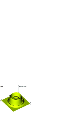
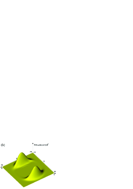
Figure 1: (Color online). The electron probability density for the initial Gaussian packet, Eqs. (24), (34): (a) at $z=0$, $k_{0}=0$ and $\Delta=5$, $d=1$ at time $t=7.5$; (b) at y=0, $k_{0}=0$ and $\Delta=5$, $d=5$ at time $t=7.5$.

In Fig.1(a) we plot the electron probability density at $z=0$ for Gaussian wave packet with initial momentum $k_{0}=0$ and $\Delta=5$, $d=1$ at time $t=7.5$. Here and below all distances are measured in units of the Compton wavelength $\lambda_{k}=\hbar/mc$, the time is in units of $t_{0}=\lambda_{k}/c$. This result was obtained by using the numerical method (”leap-frog” algorithm) described in Appendix A. Just as we expected Fig.1(a) demonstrates the axial symmetry of the considered distribution in $x,y$-plane; the probability density has a form of cylindrical wave propagating from the point of origin and having some maxima.

To analyze the motion of the packet we have to find the average value of velocity of the packet center. In the momentum representation

$$\bar{V}_{i}(t)=c\int\Psi^{+}(\vec{p},t)\alpha_{i}\Psi(\vec{p},t)d\vec{p},~{}~{}i=1,2,3.$$

Substituting Eqs.(28)-(30) into Eq.(35) and using the expressions for matrices $\alpha_{i}$ (Eq.(3)) we obtain

$$\bar{V}_{x}(t)=c\int d\vec{p}|f(\vec{p})|^{2}\Bigg{[}\frac{c^{2}p_{1}p_{3}}{\lambda_{\vec{p}}^{2}}(1-\cos\frac{2\lambda_{\vec{p}}t}{\hbar})+\frac{cp_{2}}{\lambda_{\vec{p}}}\sin\frac{2\lambda_{\vec{p}}t}{\hbar}\Bigg{]},$$

$$\bar{V}_{y}(t)=c\int d\vec{p}|f(\vec{p})|^{2}\Bigg{[}\frac{c^{2}p_{2}p_{3}}{\lambda_{\vec{p}}^{2}}(1-\cos\frac{2\lambda_{\vec{p}}t}{\hbar})-\frac{cp_{1}}{\lambda_{\vec{p}}}\sin\frac{2\lambda_{\vec{p}}t}{\hbar}\Bigg{]},$$

$$\bar{V}_{z}(t)=c\int d\vec{p}|f(\vec{p})|^{2}\Bigg{[}\frac{c^{2}p_{3}^{2}}{\lambda_{\vec{p}}^{2}}+(1-\frac{c^{2}p_{3}^{2}}{\lambda_{\vec{p}}^{2}})\cos\frac{2\lambda_{\vec{p}}t}{\hbar}\Bigg{]},$$

Since the Fourier transform $f(\vec{p})$ of Gaussian wave packet (34) has an axial symmetry in $p_{x},p_{y}$- plane

$$f(\vec{p})=\frac{d\sqrt{d}}{(\hbar\sqrt{\pi})^{3/2}}\rm e^{-\frac{p_{\bot}^{2}d^{2}}{2\hbar^{2}}-\frac{(p_{z}-\hbar k_{0})^{2}\Delta^{2}}{2\hbar^{2}}},$$

the components of velocity $\bar{V}_{x}=\bar{V}_{y}=0$ as it follows from Eqs.(36),(38). Otherwise, owing to the axial symmetry of spacial distribution of the electron density, the average coordinates of packet $\bar{x}=\bar{y}=0$. As a result, mean components of velocity in $x,y$-plane are equal to zero.

The motion of the packet center in $z$-direction experiences rapid oscillations commonly known as Zitterbewegung (the second term in square brackets in Eq.(38)). Besides, the wave packet displaces slowly with constant velocity $\bar{V}_{z0}$ (the first term in square brackets in Eq.(38); see also Eq.(B.8)) even if its momentum $\bar{p}_{z}=\hbar k_{0}=0$.

The existence of the constant component of average velocity $\bar{V}_{z0}$ in this case can be understood from the relation between velocity and momentum depending on the sign of energy: for the wave packet consisting of the states with positive (negative) energy a positive momentum $p_{z}$ corresponds to a positive (negative) velocity $V_{z}$. Let us represent the time-independent probability density in the momentum space $|\Psi(\vec{p})|^{2}$ as a superposition of the positive energy part $\Psi_{+}(\vec{p})$ and the negative energy part $\Psi_{-}(\vec{p})$

$$|\Psi(\vec{p})|^{2}=|\Psi_{+}(\vec{p})|^{2}+|\Psi_{-}(\vec{p})|^{2},$$

where $|\Psi_{\pm}(\vec{p})|^{2}=\sum\limits_{i=1}^{4}|\Psi_{i\pm}(\vec{p},t)|^{2}$, $\Psi_{i\pm}(\vec{p},t)\propto\rm e^{\mp i\frac{\lambda_{p}t}{\hbar}}$. Using Eqs.(28)-(30) one may readily show that

$$|\Psi_{\pm}(\vec{p})|^{2}=\frac{|f(\vec{p})|^{2}}{2}(1\pm\frac{cp_{z}}{\lambda_{\vec{p}}}),$$

Fig.2 shows the dependence $W_{\pm}(p_{z})=2\pi\int\limits_{0}^{\infty}|\Psi_{\pm}(\vec{p})|^{2}p_{\bot}dp_{\bot}$ (in arbitrary units) on $p_{z}$ (in units of $mc$) for the Gaussian initial wave packet, Eqs. (24), (39) for $k_{0}=0$ (a) and for $k_{0}=1$ (in units of $mc/\hbar$) (b).

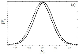
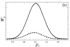
Figure 2: (Color online). The dependencies $W_{\pm}(p_{z})$ of positive (solid line) and negative (dashed line) energy parts for Gaussian initial wave packet, Eqs. (24), (39) for $k_{0}=0$, $\Delta=5$, $d=1$ (a), and for $k_{0}=1$, $\Delta=5$, $d=5$ (b).

We see that for the case $k_{0}=0$ the momentum distribution for positive- and negative- energy components is shifted towards positive and negative momentum $p_{z}$, respectively. But in both cases such dependence leads to the motion of each parts (and the whole wave packet) with a positive velocity along $z$-axis. We also see in Fig. 2(a) that the function $W_{+}(p_{z})$ has essential overlap with the function $W_{-}(p_{z})$ that is a necessary condition for existence of Zitterbewegung of the packet center (see Eq.(38)). The value of constant component of velocity $\bar{V}_{z0}$ depends on the ratio between the initial width of the wave packet and the Compton wavelength. In the limiting case $d>>1$ $\bar{V}_{z0}$ is much less than the light velocity: $\bar{V}_{z0}=\frac{c}{2}(\frac{1}{d})^{2}$. In particular, for the symmetrical wave packet ($k_{0}=0$) of width $d=\Delta=5$ $\bar{V}_{z0}\approx 0.02c$.

Let now the initial wave function $F(\vec{r})$ describes the wave packet moving along $z$-axis with average momentum $\bar{p}_{z}=\hbar k_{0}$. Then the distribution of the full electron density in $x,y$-plane is similar to one shown in Fig.1(a). However the essential difference appears in the character of evolution of the wave packet in $x,z$ (or $y,z$)-plane (Fig. 1(b)). The dependencies $W_{\pm}(p_{z})$ for the states with positive- and negative- energy parts for this case is shown in Fig. 2(b). We see that both components consist of positive momentum $p_{z}$. For the smaller negative-energy parts, this corresponds to the motion with negative velocity along $z$-axis. Thus in the position space the initial wave packet splits into two packets propagating in the opposite directions along $z$ axis.

ii) Asymmetrical wave packet evolution

We next consider another example of the initial spin polarization of the electron

$$\Psi(\vec{r},0)=\frac{F(\vec{r})}{\sqrt{2}}\pmatrix{1\cr 0\cr 0\cr 1},$$

where as before the function $F(\vec{r})$ is determined by Eq.(34).

Note that the example under review is invariant with respect to the reflection transformation $z\rightarrow-z$, i.e. the expression (42) satisfies Eq.(13). As was shown above this means that the probability density is an even function of $z$ at all times. Performing the same kind of calculations as for symmetrical wave packet we find the components of the initial wave function (42) at $t>0$ in the momentum space.

$$\halign{\hbox to\displaywidth{$\hfil\displaystyle#\hfil$}\cr 0.0pt{\hfil$\displaystyle\Psi_{1}(\vec{p},t)=\frac{f(\vec{p})}{2\sqrt{2}}\Bigg{[}e^{-i\lambda_{\vec{p}}t/\hbar}(1+\frac{mc^{2}+c(p_{1}-ip_{2})}{\lambda_{\vec{p}}})+\cr 0.0pt{\hfil$\displaystyle\hfill+\rm e^{i\lambda_{\vec{p}}t/\hbar}(1-\frac{mc^{2}+c(p_{1}-ip_{2})}{\lambda_{\vec{p}}})\Bigg{]},\hfill\hbox to0.0pt{\hss(43)}\cr}}}$$

$$\Psi_{2}(\vec{p},t)=-\Psi_{3}(\vec{p},t)=\frac{icf(\vec{p})p_{3}}{\lambda_{\vec{p}}\sqrt{2}}\sin\frac{\lambda_{\vec{p}}t}{\hbar},$$

$$\halign{\hbox to\displaywidth{$\hfil\displaystyle#\hfil$}\cr 0.0pt{\hfil$\displaystyle\Psi_{4}(\vec{p},t)=\frac{f(\vec{p})}{2\sqrt{2}}\Bigg{[}\rm e^{-i\lambda_{\vec{p}}t/\hbar}(1-\frac{mc^{2}-c(p_{1}+ip_{2})}{\lambda_{\vec{p}}})+\cr 0.0pt{\hfil$\displaystyle\hfill+\rm e^{i\lambda_{\vec{p}}t/\hbar}(1+\frac{mc^{2}-c(p_{1}+ip_{2})}{\lambda_{\vec{p}}})\Bigg{]}.\hfill\hbox to0.0pt{\hss(45)}\cr}}}$$

The components of $\Psi(\vec{r},t)$ can be obtained directly by the Fourier transform of Eqs.(43)-(45).

$$\halign{\hbox to\displaywidth{$\hfil\displaystyle#\hfil$}\cr 0.0pt{\hfil$\displaystyle\Psi_{1}(\rho,\alpha,t)=\frac{1}{2\sqrt{\pi\hbar^{3}}}\int\limits_{-\infty}^{+\infty}\rm e^{\frac{ip_{z}z}{\hbar}}dp_{z}\int\limits_{0}^{\infty}f(p_{\bot},p_{z})p_{\bot}\times\cr 0.0pt{\hfil$\displaystyle\hfill\times\Bigg{[}\cos\frac{\lambda_{\vec{p}}t}{\hbar}J_{0}(\frac{p_{\bot}\rho}{\hbar})+\frac{cp_{\bot}}{\lambda_{\vec{p}}}\sin\frac{\lambda_{\vec{p}}t}{\hbar}\rm e^{-i\alpha}J_{1}(\frac{p_{\bot}\rho}{\hbar})-\hfill\cr 0.0pt{\hfil$\displaystyle\hfill-\frac{imc^{2}}{\lambda_{\vec{p}}}\sin\frac{\lambda_{\vec{p}}t}{\hbar}J_{0}(\frac{p_{\bot}\rho}{\hbar})\Bigg{]}dp_{\bot},\hfill\hbox to0.0pt{\hss(46)}\cr}}}}$$

$$\halign{\hbox to\displaywidth{$\hfil\displaystyle#\hfil$}\cr 0.0pt{\hfil$\displaystyle\Psi_{2}(\rho,z,t)=-\Psi_{3}(\rho,z,t)=\frac{ic}{2\sqrt{\pi\hbar^{3}}}\int\limits_{-\infty}^{+\infty}p_{z}\rm e^{\frac{ip_{z}z}{\hbar}}dp_{z}\times\cr 0.0pt{\hfil$\displaystyle\hfill\times\int\limits_{0}^{\infty}f(p_{\bot},p_{z})\frac{p_{\bot}}{\lambda_{\vec{p}}}\sin\frac{\lambda_{\vec{p}}t}{\hbar}J_{0}(\frac{p_{\bot}\rho}{\hbar})dp_{\bot},\hfill\hbox to0.0pt{\hss(47)}\cr}}}$$

$$\halign{\hbox to\displaywidth{$\hfil\displaystyle#\hfil$}\cr 0.0pt{\hfil$\displaystyle\Psi_{4}(\rho,\alpha,t)=\frac{1}{2\sqrt{\pi\hbar^{3}}}\int\limits_{-\infty}^{+\infty}\rm e^{\frac{ip_{z}z}{\hbar}}dp_{z}\int\limits_{0}^{\infty}f(p_{\bot},p_{z})p_{\bot}\times\cr 0.0pt{\hfil$\displaystyle\hfill\times\Bigg{[}\cos\frac{\lambda_{\vec{p}}t}{\hbar}J_{0}(\frac{p_{\bot}\rho}{\hbar})+\frac{cp_{\bot}}{\lambda_{\vec{p}}}\sin\frac{\lambda_{\vec{p}}t}{\hbar}\rm e^{i\alpha}J_{1}(\frac{p_{\bot}\rho}{\hbar})+\hfill\cr 0.0pt{\hfil$\displaystyle\hfill+\frac{imc^{2}}{\lambda_{\vec{p}}}\sin\frac{\lambda_{\vec{p}}t}{\hbar}J_{0}(\frac{p_{\bot}\rho}{\hbar})\Bigg{]}dp_{\bot}.\hfill\hbox to0.0pt{\hss(48)}\cr}}}}$$

Using these expressions one may find the full electron density $|\Psi(\vec{r},t)|^{2}$. Figure 3(a) shows the corresponding probability density distribution in the plane $z=0$ at time $t=2\pi$. The parameters of wave packet are: $k_{0}=0$ and $\Delta=5$, $d=1$. Comparing Figs. 1(a) and 3(a) we see that the change of initial spin polarization leads to the fact that the wave packet being axially symmetric in $x,y$-plane at $t=0$ loses its symmetry at $t>0$.

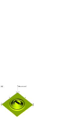
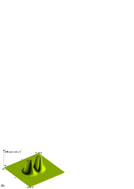
Figure 3: (Color online). The electron probability density for the initial Gaussian packet, Eqs. (42), (34): (a) at $z=0$ with $k_{0}=0$ and $\Delta=5$, $d=1$ at time $t=2\pi$; (b) at y=0, $k_{0}=1$ and $\Delta=5$, $d=2.5$ at time $t=7.5$.

The kinematics of the wave packet can be characterized by the average velocity of its center with components

$$\bar{V}_{x}(t)=c\int d\vec{p}|f(\vec{p})|^{2}\Bigg{[}\frac{c^{2}p_{1}^{2}}{\lambda_{\vec{p}}^{2}}+(1-\frac{c^{2}p_{1}^{2}}{\lambda_{\vec{p}}^{2}})\cos\frac{2\lambda_{\vec{p}}t}{\hbar}\Bigg{]},$$

$$\bar{V}_{y}(t)=c\int d\vec{p}|f(\vec{p})|^{2}\Bigg{[}\frac{c^{2}p_{1}p_{2}}{\lambda_{\vec{p}}^{2}}(1-\cos\frac{2\lambda_{\vec{p}}t}{\hbar})+\frac{mc^{2}}{\lambda_{\vec{p}}}\sin\frac{2\lambda_{\vec{p}}t}{\hbar}\Bigg{]},$$

$$\bar{V}_{z}(t)=c\int d\vec{p}|f(\vec{p})|^{2}\frac{c^{2}p_{1}p_{3}}{\lambda_{\vec{p}}^{2}}\Bigg{[}1-\cos\frac{2\lambda_{\vec{p}}t}{\hbar}\Bigg{]}.$$

As in the previous case the wave packet center drifts with constant velocity (the first term in square brackets in Eq.(49)), but now it is directed along $x$ axis. Besides, one can see from Eqs. (49) and (50) that the packet center performs damped oscillations (Fig. 4) along $x$ and $y$ directions. We also see from Eq.(51) that $\bar{V}_{z}=0$ that is the result of the symmetry under the replacement $z\rightarrow-z$, Eq.(14).

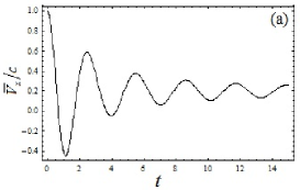
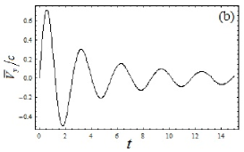
Figure 4: (Color online). The average projections of velocities $\bar{V}_{x}/c$ (a) and $\bar{V}_{y}/c$ (b) versus time $t$ (in units of $\lambda_{k}/c$) for Gaussian initial wave packet, Eqs. (42), (34) with $k_{0}=0$ and $\Delta=5$, $d=1$.

We now consider the behavior of the initial wave packet with nonzero momentum $p_{z}=\hbar k_{0}$. Obviously such initial state is not an eigenfunction of the parity operator $\hat{P}_{z}$. Nevertheless, the probability density remain to be a symmetrical function relatively to the reflection transform $z\rightarrow-z$. Indeed, one may check that the Dirac equation (1) is invariant under the transformation

$$\Psi(\vec{r},t)\rightarrow\Psi^{\prime}(x,y,z,t)=\alpha_{x}\Psi^{*}(x,y,-z,t).$$

So that if the initial wave function satisfies the equation

$$\alpha_{x}\Psi^{*}(x,y,-z,0)=\Psi(x,y,z,0),$$

then, as one can check using Eqs.(46)-(48), this relationship is valid at $t>0$ and consequently Eq. (14) holds.

The character of the motion of the packet center in $x,y$-plane is similar to the case $k_{0}=0$. Namely, the center of the wave packet drifts along $x$-direction with constant component of velocity and oscillates along $x$ and $y$ axis (Zitterbewegung). As it known the ZB is significant if the subpackets with positive and negative energy have overlap in the position space. But if the initial average momentum of the wave packet is nonzero, both subpackets move with the opposite velocities along $z$ axis that leads to their spatial separation. So, the amplitude of the ZB decreases more rapidly than for the case $k_{0}=0$ (compare Fig. 4 and Fig. 5). Notice that this result is valid for the narrow enough wave packets with width $d\leq 1$ and $dk_{0}\ll 1$ (for very large $d$ the ZB oscillations are almost undamped). The constant component of packet center velocity $\bar{V}_{x0}$ also depends on the initial momentum $\hbar k_{0}$. In fact, as it follows from Eq. (49) it decreases as $k_{0}$ increases.

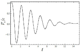
Figure 5: (Color online). The average projection of velocity $\bar{V}_{x}/c$(a) versus time $t$ (in units of $\lambda_{k}/c$) for Gaussian initial wave packet, Eqs. (42), (34) with $k_{0}=1$ and $\Delta=5$, $d=2.5$.

IV Spin dynamics

At present we consider the average value of the spin operator $\vec{\Sigma}$ for Dirac particle

$$\bar{\Sigma}_{\mu}(t)=\int d\vec{r}\Sigma_{\mu}(\vec{r},t)=\int d\vec{r}\sum\limits_{i=1}^{4}\Psi_{i}^{+}(\vec{r},t)\Sigma_{\mu}\Psi_{i}(\vec{r},t),$$

or in the momentum representation

$$\bar{\Sigma}_{\mu}(t)=\int d\vec{p}\sum\Psi_{i}^{+}(\vec{p},t)\Sigma_{\mu}\Psi_{i}(\vec{p},t).$$

One can verify that the spin densities $\Sigma_{\mu}(\vec{r},t)$ for the arbitrary wave function with components $\Psi_{i}=\Psi_{i}(\vec{r},t)$ are

$$\Sigma_{x}(\vec{r},t)=2{\rm Re}(\Psi_{1}^{*}\Psi_{2}+\Psi_{3}^{*}\Psi_{4}),$$

$$\Sigma_{y}(\vec{r},t)=2{\rm Im}(\Psi_{1}^{*}\Psi_{2}+\Psi_{3}^{*}\Psi_{4}),$$

$$\Sigma_{z}(\vec{r},t)=|\Psi_{1}|^{2}-|\Psi_{2}|^{2}+|\Psi_{3}|^{2}-|\Psi_{4}|^{.}$$

i) Cylindrically symmetric wave packet

The form of Eqs.(55)-(57) and the expressions (31)-(33) for the components of wave function show that for an axially symmetric wave packet, Eq.(24) the component of spin density $\Sigma_{z}$ is an axially symmetric too both for $k_{0}=0$ and $k_{0}\neq 0$ (Fig. 6(c)). One can also verify that $\Sigma_{x}$ and $\Sigma_{y}$ components can be written in the form

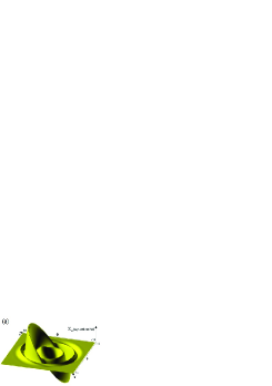
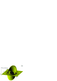
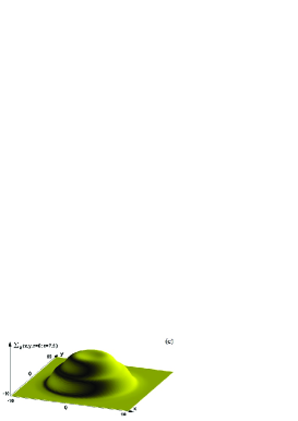
Figure 6: (Color online). The distributions of the components of spin density $\Sigma_{x}(x,y,0,t)$, $\Sigma_{y}(x,y,0,t)$, $\Sigma_{z}(x,y,0,t)$ for initial Gaussian packet, Eqs. (24), (34) with $k_{0}=0$ and $\Delta=5$, $d=1$ at time $t=7.5$.

$$\Sigma_{x}=x\cdot g(\rho,z,t),~{}~{}~{}\Sigma_{y}=y\cdot g(\rho,z,t),$$

where the expression for the function $g(\rho,z,t)$ is enough cumbrous and will not be presented here. Thus the $x,y$-plane projection of vector $\vec{\Sigma}(\vec{r},t)$ is directed along the unit vector of cylindrical system $\vec{e}_{\rho}$. The spin densities $\Sigma_{x}(x,y,0,t)$ and $\Sigma_{y}(x,y,0,t)$ are represented in Fig. 6(a),(b) for the Gaussian wave packet with the average momentum $\bar{p}_{z}=\hbar k_{0}=0$. We see that $\Sigma_{x}(x,y,0,t)$ ($\Sigma_{y}(x,y,0,t)$) is the antisymmetrical function of $x$($y$) and the spin density $\Sigma_{z}(x,y,0,t)$ conserves its axial symmetry.

The average values of spin operators for this polarization can be found by using Eqs.(28)-(30) for wave function in the momentum representation and previous definition, Eq.(54b).

$$\bar{\Sigma}_{x}(t)=\int\frac{|f(\vec{p})|^{2}}{\lambda_{\vec{p}}^{2}}\Bigg{[}cp_{2}\lambda_{\vec{p}}\sin\frac{2\lambda_{\vec{p}}t}{\hbar}+c^{2}p_{3}p_{1}(1-\cos\frac{2\lambda_{\vec{p}}t}{\hbar})\Bigg{]}d\vec{p},$$

$$\bar{\Sigma}_{y}(t)=\int\frac{|f(\vec{p})|^{2}}{\lambda_{\vec{p}}^{2}}\Bigg{[}-cp_{1}\lambda_{\vec{p}}\sin\frac{2\lambda_{\vec{p}}t}{\hbar}+c^{2}p_{3}p_{2}(1-\cos\frac{2\lambda_{\vec{p}}t}{\hbar})\Bigg{]}d\vec{p},$$

$$\bar{\Sigma}_{z}(t)=\int\frac{|f(\vec{p})|^{2}}{\lambda_{\vec{p}}^{2}}\Bigg{[}(\lambda_{\vec{p}}^{2}-c^{2}p_{\bot}^{2})+c^{2}p_{\bot}^{2}\cos\frac{2\lambda_{\vec{p}}t}{\hbar}\Bigg{]}d\vec{p}.$$

As it follows from these relations only $\bar{\Sigma}_{z}(t)$ is not equal to zero for the considered wave packet. The first term in square brackets of the last formula corresponds to the constant component of $\bar{\Sigma}_{z}(t)$ and the second one describes the typical transient Zitterbewegung.

ii) Asymmetrical wave packet

One can easy verify that the second example, Eq.(42) considered in our work corresponds to the initial spin density $\vec{\Sigma}(\vec{r},0)=0$. Really, as it follows from Eqs.(46)-(48) the components of wave function for the packet with $k_{0}=0$ at $z=0$ obey the relations

$$\halign{\hbox to\displaywidth{$\hfil\displaystyle#\hfil$}\cr 0.0pt{\hfil$\displaystyle\Psi_{1}^{*}(x,y,0,t)=\Psi_{4}(x,y,0,t),\cr 0.0pt{\hfil$\displaystyle\hfill\Psi_{2}^{*}(x,y,0,t)=\Psi_{3}(x,y,0,t)=0,\hfill\crcr}}}$$

that together with Eqs.(55)-(57) leads to the result $\Sigma_{x}(x,y,0,t)=\Sigma_{y}(x,y,0,t)=\Sigma_{z}(x,y,0,t)=0$.

The analysis of expressions (46)-(48) and (57) shows that in $x,z$-plane the $z$-component of spin density is an antisymmetric function of $z$ that is connected with discussed above symmetry of probability density with respect to the replacement $z\rightarrow-z$.

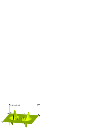
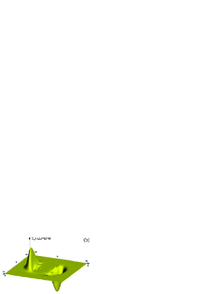
Figure 7: (Color online). The distributions of the components of spin density $\Sigma_{x}(x,0,z,t)$, $\Sigma_{y}(x,0,z,t)$ for initial Gaussian packet, Eqs. (42), (34) with $k_{0}=0$ and $\Delta=d=3.64$ at time $t=8$.

Fig. 7 illustrates the distributions of $\Sigma_{x}(x,0,z,t)$ and $\Sigma_{z}(x,0,z,t)$ for Gaussian wave packet with $k_{0}=1$ and $\Delta=d=3.64$, at $t=8$.

By inserting Eqs.(43)-(45) into Eq.(54b) we find for the average components of spin

$$\bar{\Sigma}_{x}(t)=-\int\frac{|f(\vec{p})|^{2}}{\lambda_{\vec{p}}^{2}}mc^{3}p_{3}(1-\cos\frac{2\lambda_{\vec{p}}t}{\hbar})d\vec{p},$$

$$\bar{\Sigma}_{y}(t)=\int\frac{|f(\vec{p})|^{2}}{\lambda_{\vec{p}}}cp_{3}\sin\frac{2\lambda_{\vec{p}}t}{\hbar}d\vec{p}.$$

$$\halign{\hbox to\displaywidth{$\hfil\displaystyle#\hfil$}\cr 0.0pt{\hfil$\displaystyle\bar{\Sigma}_{z}(t)=\int\frac{|f(\vec{p})|^{2}}{\lambda_{\vec{p}}}\Bigg{[}-cp_{2}\sin\frac{2\lambda_{\vec{p}}t}{\hbar}+\frac{mc^{3}p_{1}}{\lambda_{\vec{p}}}\times\cr 0.0pt{\hfil$\displaystyle\hfill\times(1-\cos\frac{2\lambda_{\vec{p}}t}{\hbar})\Bigg{]}d\vec{p}.\hfill\hbox to0.0pt{\hss(64)}\cr}}}$$

Obviously for a symmetric wave function $f(\vec{p})=f(-\vec{p})$ (that means $k_{0}=0$) these expressions give $\bar{\Sigma}_{x}=\bar{\Sigma}_{y}=\bar{\Sigma}_{z}=0$. Note that $\bar{\Sigma}_{z}$ remains to be equal to zero also for $\bar{p}_{z}=\hbar k_{0}\neq 0$. It may be shown that in this case Eqs.(62),(63) describe the spin ”precession” (in $x,y$-plane about vector $\vec{k_{0}}$) which has a transient character. Such phenomenon for a hole system, described by Luttinger model was discussed in the recent work of authors.DMF

V Summary

In this work we have studied the quantum dynamics of relativistic particles represented by three-dimensional Gaussian wave packets with different initial spin polarizations, described by the Dirac equation. The analysis of the general symmetry properties of solutions of one-particle Dirac equation allows to predict the direction of average electron velocity as well as the direction of trembling motion. In particular, the evolution of spherically and cylindrically symmetric initial Gaussian wave packet demonstrates that the wave packet with initial polarization, which is determined by bispinor $\pmatrix{1&0&1&0}^{T}$ has cylindrical symmetry at all times $t>0$, but the wave packet with initial polarization $\pmatrix{1&0&0&1}^{T}$ loses its cylindrical symmetry at time $t>0$. The influence of the symmetry of initial wave packet on the distribution of spin densities is analyzed.

Appendix A

The ”leap-frog” algorithmS is applied in a spatial grid of bin-sizes $\Delta x$, $\Delta y$, $\Delta z$ and with time step $\Delta t$:

$$\Psi(\vec{r},t+2\Delta t)=\Psi(\vec{r},t)-2i\Delta t\hat{H}(\vec{r})\Psi(\vec{r},t+\Delta t),$$

The spatial derivatives are computed symmetrically. Reflecting boundary conditions are applied on a very large grid (running stops before reflections occur if necessary). We use the norm as the stability measure of the algorithm (1). In accordance with von Neumann stability analysisGKO (for large component plane waves) the stability region ($d$-spatial grid bin, $\Delta t$-time step) is:

$$d^{4}\Bigg{(}1-(\Delta t)^{2}\Bigg{)}-2(d\Delta t)^{2}-4(\Delta t)^{2}>0,$$

Thus, for a single precision calculation the loss of norm can be kept within $10^{-7}$-$10^{-6}$ in a $10^{3}$ time step run. It should be noted that in the case of Zitterbewegung, i.e. of the spatial oscillation of the wave packet, one more condition have to be imposed to the lattice sizes:

$$\Delta x\sim\Delta y\sim\Delta z<\frac{\hbar}{mc},$$

The conditions (A.2) and (A.3) were fulfilled in all our calculations.

Appendix B. Drift velocity for the arbitrary initial wave function

As was shown in previous investigations the motion of the Dirac wave packet center does not obey classical relativistic kinematics. In particular, besides the rapid oscillations (ZB) the wave packet can drift with constant velocity although its average momentum is zero. One can show that in this case the direction of such motion coincides with the direction of initial average velocity. In fact, for the second example considered in this work (Eq. (42)) only $\bar{V}_{x}(t=0)=c$ and $\bar{V}_{y}(t=0)=\bar{V}_{z}(t=0)=0$. Therefore such initial spin polarization leads to the motion of the wave packet with constant velocity along $x$ axis (see Eqs. (21),(26)). It is easy to see that in the first example, Eq. (10), the wave packet at $t=0$ has the velocity directed along $z$ axis, so the motion at $t>0$ occurs in this direction.

Let now find the drift velocity of particle for the case of arbitrary initial polarization

$$\Psi(\vec{p},t)=Af(\vec{p})\pmatrix{\varphi_{1}\cr\varphi_{2}\cr\varphi_{3}\cr\varphi_{4}},$$

where $\varphi_{i}$ are the complex coefficients, $A=\frac{1}{\sqrt{\sum\limits_{i}|\varphi_{i}|^{2}}}$, and $f(\vec{p})$ is to be determined from the Fourier expansion of coordinate wave function $F(\vec{r})$. (We do not suppose that $F(\vec{r})$ and $f(\vec{p})$ have any symmetry).

At $t>0$ the wave function in momentum representation is

$$\halign{\hbox to\displaywidth{$\hfil\displaystyle#\hfil$}\cr 0.0pt{\hfil$\displaystyle\Psi(\vec{p},t)=\Psi_{+}(\vec{p},t)+\Psi_{-}(\vec{p},t)=\cr 0.0pt{\hfil$\displaystyle\hfill\sum\limits_{i=1}^{2}C_{i}(\vec{p})U_{i}(\vec{p})\rm e^{-i\lambda_{\vec{p}}t/\hbar}+\sum\limits_{i=3}^{4}C_{i}(\vec{p})U_{i}(\vec{p})\rm e^{i\lambda_{\vec{p}}t/\hbar},~{}\hfill\hbox to0.0pt{\hss(B.2)}\cr}}}$$

Using the Eqs (5),(6) and (8) for free Dirac spinors we find from Eq. (B.2)

$$\halign{\hbox to\displaywidth{$\hfil\displaystyle#\hfil$}\cr 0.0pt{\hfil$\displaystyle C_{1}=Af(\vec{p})N(\varphi_{1}+\gamma(p_{1}-ip_{2})\varphi_{4}+\gamma p_{3}\varphi_{3}),\cr 0.0pt{\hfil$\displaystyle\hfill C_{2}=Af(\vec{p})N(\varphi_{2}+\gamma(p_{1}+ip_{2})\varphi_{3}-\gamma p_{3}\varphi_{4}),\hfill\cr 0.0pt{\hfil$\displaystyle\hfill C_{3}=Af(\vec{p})N(-\gamma p_{3}\varphi_{1}-\gamma(p_{1}-ip_{2})\varphi_{2}+\varphi_{3}),\hfill\cr 0.0pt{\hfil$\displaystyle\hfill C_{4}=Af(\vec{p})N(-\gamma(p_{1}+ip_{2})\varphi_{1}+\gamma p_{3}\varphi_{2}+\varphi_{4}).\hfill\hbox to0.0pt{\hss(B.3)}\cr}}}}}$$

The density of $\mu$-component of velocity ($\mu=1,2,3$) in the momentum space is

$$V_{\mu}(\vec{p},t)=\Psi^{+}(\vec{p},t)\hat{V}_{\mu}\Psi(\vec{p},t),~{}~{}\hat{V}_{\mu}=c\alpha_{\mu}.$$

Obviously the time-independent part $V_{\mu 0}$ of $V_{\mu}(\vec{p},t)$ is defined as

$$V_{\mu 0}(\vec{p})=\Psi_{+}^{+}(\vec{p},t)\hat{V}_{\mu}\Psi_{+}(\vec{p},t)+\Psi_{-}^{+}(\vec{p},t)\hat{V}_{\mu}\Psi_{-}(\vec{p},t),$$

where $\Psi_{+}(\vec{p},t)$ and $\Psi_{-}(\vec{p},t)$ corresponds to the contribution of positive and negative energy into Eq.(B.2). One may check that

$$(V_{\mu})_{ij}=U_{i}\hat{V}_{\mu}U_{j}=\Bigg{\{}{\frac{cp_{\mu}}{\lambda_{\vec{p}}}\delta_{ij},~{}i,j=1,2\atop-\frac{cp_{\mu}}{\lambda_{\vec{p}}}\delta_{ij},~{}i,j=3,4}.$$

So, using Eqs. (B.2), (B.5) and (B.6) we obtain

$$\bar{V}_{\mu 0}=\int\frac{c^{2}p_{\mu}}{\lambda_{\vec{p}}^{2}}(|C_{1}|^{2}+|C_{2}|^{2}-|C_{3}|^{2}-|C_{4}|^{2})d\vec{p}.$$

Substituting the expression for the coefficients $C_{i}$, Eq.(B.3) into the Eq.(B.7), we find the constant velocity of wave packet center

$$\halign{\hbox to\displaywidth{$\hfil\displaystyle#\hfil$}\cr 0.0pt{\hfil$\displaystyle\bar{V}_{\mu 0}=\frac{c}{\sum\limits_{i=1}^{4}|\varphi_{i}|^{2}}\int|f(\vec{p})|^{2}\frac{c^{2}p_{\mu}}{\lambda_{\vec{p}}^{2}}\Bigg{[}mc(|\varphi_{1}|^{2}+|\varphi_{2}|^{2}-|\varphi_{3}|^{2}-|\varphi_{4}|^{2})\cr 0.0pt{\hfil$\displaystyle\hfill+2p_{1}{\rm Re}(\varphi_{1}^{*}\varphi_{4}+\varphi_{3}^{*}\varphi_{2})+2p_{2}{\rm Im}(\varphi_{1}^{*}\varphi_{4}+\varphi_{3}^{*}\varphi_{2})+\hfill\cr 0.0pt{\hfil$\displaystyle\hfill+2p_{3}{\rm Re}(\varphi_{1}^{*}\varphi_{3}-\varphi_{2}^{*}\varphi_{4})\Bigg{]}.\hfill\hbox to0.0pt{\hss(B.8)}\cr}}}}$$

It is convenient to represent this expression using the initial components of velocity $\bar{V}_{\mu}(0)$, so that

$$\halign{\hbox to\displaywidth{$\hfil\displaystyle#\hfil$}\cr 0.0pt{\hfil$\displaystyle\bar{V}_{\mu 0}=\bar{V}_{\mu}(0)\int|f(\vec{p})|^{2}\frac{p_{\mu}^{2}}{\lambda_{\vec{p}}^{2}}d\vec{p}+mc^{4}\int|f(\vec{p})|^{2}\frac{p_{\mu}}{\lambda_{\vec{p}}^{2}}\times\cr 0.0pt{\hfil$\displaystyle\hfill\times\frac{(|\varphi_{1}|^{2}+|\varphi_{2}|^{2}-|\varphi_{3}|^{2}-|\varphi_{4}|^{2})}{\sum\limits_{i=1}^{4}|\varphi_{i}|^{2}}d\vec{p}.\hfill\hbox to0.0pt{\hss(B.9)}\cr}}}$$

(Note that in this equation there is no summation over $\mu$). Let the initial Gaussian wave packet be spherically symmetric, i.e. $f(\vec{p})$ is determined by Eq.(39) with $d=\Delta$. Then if the average momentum $\hbar k_{0}=0$ the second term in Eq.(B.9) equals to zero and the value of integral in the first term does not depend on $\mu$. Thus the direction of the constant velocity of wave packet coincides with the initial one. In the case $k_{0}d>>1$ as it follows from Eq.(B.9) $\bar{V}_{z0}>>\bar{V}_{x0}$, $\bar{V}_{y0}$ and the asymptotic direction of the average velocity is along $z$-axis, i.e. along the average momentum $\bar{p}_{z}=\hbar k_{0}$. A similar result was obtained in our previous workMDF , concerning the propagation of the wave packet in graphene.

Note that Eq.(A.8) is valid also for the most general initial wave packet of the form

$$\Psi(\vec{p},0)=(\Psi_{1}(\vec{p}),\Psi_{2}(\vec{p}),\Psi_{3}(\vec{p}),\Psi_{4}(\vec{p}))^{T},$$

if we rename $\Psi_{i}(\vec{p})=\frac{f(\vec{p})\varphi_{i}}{\sqrt{\sum|\varphi_{i}|^{2}}}$ in Eq.(B.8) . It is not difficult to check that the expressions for the constant components of velocity obtained earlier for the examples Eq.(24) and Eq.(42) follow also from the general equation (B.8).

References

(1) E. Schrödinger, Sitzungsber. Peuss. Akad. Wiss., Phys. Math. Kl. 24, 418 (1930). See also A. O. Barut and A. J. Bracken,
where Schrödinger’s work on Zitterbewegung of the
electrons is reexamined, Phys. Rev. D 23, 2454 (1981).
(2) O. Klein, Z.Phys. 53, 157 (1929).
(3) R. Gerritsma, G. Kirchmair, F. Zähringer, E. Solano, R. Blatt , C. F. Roos, Nature 463, 68 (2010).
(4) L. Lamata, J. Leon, T. Schätz, and E. Solana, Phys. Rev. Lett. 98, 253005 (2007).
(5) B. Thaller, arXiv:quant-ph/0409079 (2004, unpublished).
(6) J. A. Lock, Am. J. Phys. 47, 797 (1979).
(7) N. Simicevic, arXiv: 0812.1807v1 [physics.comp-ph] (2008); N. Simicevic, arXiv: 0901.3765v1 [quant-ph] (2009).
(8) P. Krekora, Q. Su, and R. Grobe, Phys. Rev. Lett. 93, 043004 (2004).
(9) L. Ferrari and G. Russo, Phys. Rev. B 42, 7454 (1990).
(10) J. Schliemann, D. Loss, and R. M. Westervelt, Phys. Rev. Lett. 94, 206801 (2005).
(11) V. Ya. Demikhovskii, G. M. Maksimova, and E. V. Frolova, Phys. Rev. B 78, 115401 (2008).
(12) W. Zawadzki, Phys. Rev. B 72, 085217 (2005).
(13) M. Katsnelson, Eur. Phys. J. B 51, 157 (2006).
(14) T. M. Rusin and W. Zawadzki, Phys. Rev. B 76, 195439 (2007).
(15) G. M. Maksimova, V. Ya. Demikhovskii, and E. V. Frolova, Phys. Rev. B 78, 235321 (2008).
(16) D. Lurie and S. Cremer, Physica (Amsterdam) 50, 224 (1970).
(17) J. J. Sakurai, Advanced Quantum Mechanics, Addison-Wesly, Reading,
MA, 92, (1967).
(18) V. Ya. Demikhovskii, G. M. Maksimova, and E. V. Frolova, Phys. Rev. B 81, 115206 (2010).
(19) U. Schumann, J. Comput. Phys. 18, N. 4, 465 (1975).
(20) B. Gustafsson , H.-O. Kreiss , J. Oliger, Time Dependent Problems and Difference methods, Wiley, N.Y. (1995).