Improving beam stability in particle accelerator models by using Hamiltonian control

Abstract

We derive a Hamiltonian control theory which can be applied to a 4D symplectic map that models a ring particle accelerator composed of elements with sextupole nonlinearity. The controlled system is designed to exhibit a more regular orbital behavior than the uncontrolled one. Using the Smaller Alignement Index (SALI) chaos indicator, we are able to show that the controlled system has a dynamical aperture up to $1.7$ times larger than the original model.

1 Introduction

Particle accelerators are technological devices which allow studies at both “infinitely small scale”, e.g. particles responsible for elementary forces, and “extremely large scale”, e.g. the origin of cosmos. In a simplified approach, such devices are composed of basic elements sequence: focusing and defocusing magnets, accelerating electromagnetic fields and trajectory bending elements as they are used in the case of ring accelerators. The resulting dynamics is nonlinear, and can be described, in the absence of strong damping, by a conservative system. This system can be modelled by a symplectic map built from the composition of several elementary maps corresponding to each basic magnetic element.

One of the main problems found in the dynamics of ring accelerators is to study the stability around the nominal orbit, i.e. the circular orbit passing through the centre of the ring. Each component of the ring can be seen as a nonlinear map, that deforms the trajectory at large amplitude. Moreover, such maps possess stochastic layers whose effect is the reduction of the stability domains around the nominal circular orbit (the so-called dynamical aperture - DA) [1]. Such behaviors imply that (chaotic) nearby orbits can drift away after a few ring turns, eventually colliding with accelerator’s boundaries, and consequently reduce the beam lifetime and the performance of the accelerator.

The aim of the present paper is to derive a reliable improvement of the stability of the beam by increasing the DA in a simplified accelerator model, consisting of only one type of element having a sextupole nonlinearity [2, 3, 4, 5].

We work in the framework of the Hamiltonian Control Theory presented in [7, 8], where two methods to control symplectic maps have been described, namely using Lie transformations and generating functions. In the present paper we use the former method, that allows direct determination of the new controlled map; avoiding the possible problems related to coordinate inversion.

The aim of control theory is to improve selected features of a given system, by slightly modifying its Hamiltonian with the addition of a small control term, so that the new system and the unperturbed one are conjugated namely, they have the same dynamics. This technique is particularly suitable whenever one can directly act on the system and modify it, e.g. in the case of a particle accelerator where the addition of a control term in the Hamiltonian function can be seen as the introduction of a suitable magnet in the accelerator lattice.

In our study, we use the Smaller Alignement Index (SALI) [6, 10, 11, 12] method, which is an efficient indicator for characterising orbits as chaotic or regular in Hamiltonian flows and symplectic maps. The SALI is computed using the time evolution of two deviation vectors along the studied orbit.

The paper is organized as follows: we introduce the model in Section 2 and present a general result for the control of symplectic maps in Section 3. We apply the theory to the symplectic map model of a standard ring accelerator in Section 4. We briefly recall the SALI chaos indicator in Section 5, while Section 6 presents our numerical results on the behavior of the constructed model. Finally, in Section 7 we summarize our conclusions. Further technical details can be found in the Appendix.

2 The model

Let us consider a system consisting of a charged particle and a simplified accelerator ring with linear frequencies (tunes) $q_{x}$, $q_{y}$, with a localized thin sextupole magnet (for more details the interested reader is referred to [2]). The magnetic field of this element modifies the orbit once the particle passes through it. The basic model is :

$$\left(\begin{smallmatrix}x_{1}^{\prime}\\ x_{2}^{\prime}\\ x_{3}^{\prime}\\ x_{4}^{\prime}\end{smallmatrix}\right)=\left(\begin{smallmatrix}\cos\omega_{1}&-\sin\omega_{1}&0&0\\ \sin\omega_{1}&\cos\omega_{1}&0&0\\ 0&0&\cos\omega_{2}&-\sin\omega_{2}\\ 0&0&\sin\omega_{2}&\cos\omega_{2}\\ \end{smallmatrix}\right)\left(\begin{smallmatrix}x_{1}\\ x_{2}+x_{1}^{2}-x_{3}^{2}\\ x_{3}\\ x_{4}-2x_{1}x_{3}\end{smallmatrix}\right)=T\left(\begin{smallmatrix}x_{1}\\ x_{2}\\ x_{3}\\ x_{4}\end{smallmatrix}\right)\,$$ (1)

where $x_{1}$ ($x_{3}$) denote the deflection from the ideal circular orbit in the horizontal (vertical) direction before the particle enters the element and $x_{2}$ ($x_{4}$) are the associated momentum. Primed variables denote positions and momenta after the particle left the element. The parameters $\omega_{1}$ and $\omega_{2}$ are related to the accelerator’s tunes  $q_{x}$ and $q_{y}$ by the relations $\omega_{1}=2\pi q_{x}$ and $\omega_{2}=2\pi q_{y}$. The first matrix in (1) describes the linear motion of a particle, which corresponds to a simple rotation in the phase space. The nonlinearity induced by the thin sextupole magnet is modeled by the 2^nd order polynomial expression in (1). The particle dynamics at the $n$-th turn, can be described by the sequence $(x_{1}^{(n)},x_{2}^{(n)},x_{3}^{(n)},x_{4}^{(n)})_{n\geq 0}$, where the $(n+1)$-th positions and momenta are defined as a function of the $n$-th ones by (1).

The map (1) decomposes in an integrable part and a quadratic perturbation, respectively the system is associated to the following Hamiltonian (see A)

$$H(x_{1},x_{2},x_{3},x_{4})=-\omega_{1}\frac{x_{1}^{2}+x_{2}^{2}}{2}-\omega_{2}\frac{x_{3}^{2}+x_{4}^{2}}{2}\quad\text{and}\quad V(x_{1},x_{2},x_{3},x_{4})=-\frac{x_{1}^{3}}{3}+x_{1}x_{3}^{2}\,,$$ (2)

more precisely (1) can be written in terms of Poisson brackets  as

$$\vec{x}^{\prime}=T(\vec{x})=e^{\{H\}}e^{\{V\}}\vec{x}\,.$$ (3)

Here $\vec{x}=(x_{1},x_{2},x_{3},x_{4})^{\rm T}$, with ^T denoting the transpose of a matrix, and by definition, for any function $f$ defined in the phase space, $\{H\}f=\{H,f\}=(\nabla H)^{\mathrm{T}}J\nabla f$, with $J=\left(\begin{array}[]{cc}\mathbf{0}&\mathbf{1}\\ -\mathbf{1}&\mathbf{0}\end{array}\right)$, being the symplectic constant matrix,

$$e^{\{H\}}f=\sum_{n\geq 0}\frac{\{H\}^{n}}{n!}f\quad\text{and}\quad\{H\}^{n}f=\{H\}^{n-1}(\{H\}f)\,.$$ (4)

Maps of the form (1) have already been studied in  [6] where it has been shown that chaotic orbits reduce the DA to a hypersphere of radius $\sim 0.39$ in the 4-dimensional phase space (see Figs. 5 and 6 of [6]). The goal of the present paper is to show that the stability region of the nominal circular orbit can be increased once the map (1) is controlled by an appropriately designed map.

3 Control theory for symplectic maps

The aim of Hamiltonian theory is to provide mathematic tools to be able to modify the dynamics of a symplectic system. With this, it is possible to manipulate intrinsic features, e.g. to reduce the chaotic regions in phase space or to build invariant tori.

In the following we will be interested in controlling a quasi-integrable symplectic map in such a way that it will allow us to obtain a new, controlled map “closer” to the integrable part of the original map, and thus increase the stability region around the nominal circular orbit. This is of great importance since chaos diffusion channels in phase space with unpredictable consequences in configuration space. The controlled map is expected to have a smaller number of escaping orbits and a larger region occupied by invariant curves in a neighbourhood of the origin. For this purpose, we apply the method presented in [8], with the modification that in the present case the integrable part is not expressed in action-angle variables. In particular, the integrable part is a rotation, so the present theory applies to perturbations of rotations, instead of maps close to identity.

Let us consider an integrable symplectic map defined through its infinitesimal generator  $H$

$$\vec{x}^{\prime}=e^{\{H\}}\vec{x}\,,$$ (5)

and consider the quasi-integrable map perturbation of the former

$$\vec{x}^{\prime}=T(\vec{x})=e^{\{H\}}e^{\{V\}}\vec{x}\,,$$ (6)

where $\vec{x}\in\mathbb{R}^{2N}$ and $V$ is a perturbation, namely $V=o(H)$. The aim of Hamiltonian control theory, is to construct a third map, the control map, whose generator $F$ is small (it satisfies $F=o(V)$). The controlled map

$$T_{ctrl}=e^{\{H\}}e^{\{V\}}e^{\{F\}}\,,$$ (7)

will be conjugated to a map $T_{*}$, closer to $e^{\{H\}}$ than $T$ (see (11) below). We note that the use of the exponential of a Poisson bracket, ensures that such maps are symplectic by construction.

To be more precise, let us define the unperturbed map

$$\mathcal{A}^{-1}=e^{-\{H\}}\,,$$ (8)

and observe that $(1-\mathcal{A}^{-1})$ is not invertible, since its kernel contains any smooth function of $H$. Thus we assume the existence of a “pseudo-inverse”operator, $\mathcal{G}$, that should satisfy (see [8] for details)

$$\mathcal{G}\left(1-\mathcal{A}^{-1}\right)\mathcal{G}=\mathcal{G}\,.$$ (9)

At this point we can define the non-resonant and the resonant operators

$$\mathcal{N}:=\left(1-\mathcal{A}^{-1}\right)\mathcal{G}\quad\text{and}\quad\mathcal{R}:=1-\mathcal{N}\,,$$ (10)

which are projectors, i.e. $\mathcal{N}^{2}=\mathcal{N}$ and $\mathcal{R}^{2}=\mathcal{R}$.

Our main theoretical result can be stated in the following theorem:

Theorem 3.1.

Under the above hypotheses and defining $S=\mathcal{G}V$ we have

$$e^{\{S\}}T_{ctrl}e^{-\{S\}}=e^{\{H\}}e^{\{\mathcal{R}V\}}:=T_{*}\,,$$ (11)

where

$$T_{ctrl}=e^{\{H\}}e^{\{V\}}e^{\{F\}}\,,$$ (12)

with a control term given by

$$e^{\{F\}}=e^{-\{V\}}e^{\{\left(\mathcal{N-G}\right)V\}}e^{\{\mathcal{R}V\}}e^{\{\mathcal{G}V\}}\,.$$ (13)

Remark 3.2 (Warped addition).

Let us define as in [8] the warped addition, $\{A\}\oplus\{B\}$, of two operators by

$$e^{\{A\}}e^{\{B\}}:=e^{\{A\}\oplus\{B\}}\,.$$ (14)

An explicit formula can be obtained using the Baker-Campbell-Hausdorff formula [9], where $\{A\}\oplus\{B\}$ is a series whose first terms are

$$\{A\}\oplus\{B\}=\{A\}+\{B\}+\frac{1}{2}\left(\{A\}\{B\}-\{B\}\{A\}\right)+\dots\,,$$ (15)

hence the warped addition is a deformation of the usual addition between operators.

Proof.

Using this warped addition, we can rewrite the controlled map into the form

$$T_{ctrl}=e^{\{H\}\oplus\{V\}\oplus\{F\}}\,,$$ (16)

where the control term (13) becomes

$$\{F\}=-\{V\}\oplus\{\left(\mathcal{N-G}\right)V\}\oplus\{\mathcal{R}V\}\oplus\{\mathcal{G}V\}\,.$$ (17)

From (10) we have:

$$\mathcal{N-G}=-\mathcal{A}^{-1}\mathcal{G}\,.$$ (18)

One can easily prove (see appendix A of [8]) that

$$\left(-\{H\}\right)\oplus\left(-\{S\}\right)\oplus\{H\}=-\{\mathcal{A}^{-1}S\}\,,$$ (19)

hence, recalling the definition of $S$ and (18), we can rewrite (17) as

$$\{F\}=-\{V\}\oplus(-\{H\})\oplus(-\{S\})\oplus\{H\}\oplus\{\mathcal{R}V\}\oplus\{S\}\,.$$ (20)

By rearranging the terms we can easily get

$$\{S\}\oplus\{H\}\oplus\{V\}\oplus\{F\}\oplus(-\{S\})=\{H\}\oplus\{\mathcal{R}V\}\,,$$ (21)

which is nothing but (11) rewritten using the warped addition. ∎

Remark 3.3.

Let us observe that the control term is, as required, small compared to $V$. In fact from (17) and by using the approximated formula for the warped addition (15), we obtain

$$\{F\} = -\{V\}\oplus\{\left(\mathcal{N-G}\right)V\}\oplus\{\mathcal{R}V\}\oplus\{\mathcal{G}V\}$$ (22)

$$= -\{V\}+\{\mathcal{N}V\}-\{\mathcal{G}V\}+\{\mathcal{R}V\}+\{\mathcal{G}V\}+o(V)=o(V)\,,$$ (23)

where we use the relation $\mathcal{N+R}=1$.

Under the assumption of absence of resonances, i.e. $\mathcal{R}V=0$, the $o(V)$ term in the control map can be explicitly computed to give (see A)

$$F=\frac{1}{2}\{V\}\mathcal{G}V+o(V^{2})\,.$$ (24)

4 The control term for the non-resonant map

In this section we derive the controlled map presented in section 3 in case of maps of the form (1). To implement the theory we need to diagonalize the operator $\{H\}$. For this reason we introduce complex variables

$$\zeta_{1}=x_{2}+ix_{1}\quad\text{and}\quad\zeta_{2}=x_{4}+ix_{3}\,,$$ (25)

and rewrite $H$ as

$$H(\zeta_{1},\zeta_{2})=-\frac{\omega_{1}}{2}|\zeta_{1}|^{2}-\frac{\omega_{2}}{2}|\zeta_{2}|^{2}\,.$$ (26)

The Poisson bracket with $H$ now takes the form

$$\{H\}=i\omega_{1}\left(\bar{\zeta}_{1}\partial_{\bar{\zeta}_{1}}-{\zeta}_{1}\partial_{{\zeta}_{1}}\right)+i\omega_{2}\left(\bar{\zeta}_{2}\partial_{\bar{\zeta}_{2}}-{\zeta}_{2}\partial_{{\zeta}_{2}}\right)\,.$$ (27)

Hence, for any $\vec{n}=(n_{1},n_{2})\in\mathbb{N}^{2}$ and $\vec{m}=(m_{1},m_{2})\in\mathbb{N}^{2}$ we obtain

$$\{H\}\zeta^{\vec{n}}\bar{\zeta}^{\vec{m}}=i\left(\omega_{1}m_{1}-\omega_{1}n_{1}+\omega_{2}m_{2}-\omega_{2}n_{2}\right)\zeta^{\vec{n}}\bar{\zeta}^{\vec{m}}=i\vec{\omega}\cdot(\vec{m}-\vec{n})\zeta^{\vec{n}}\bar{\zeta}^{\vec{m}}.$$ (28)

Here we introduced the vector $\vec{\omega}=(\omega_{1},\omega_{2})$ and use the compact notation $\zeta^{\vec{n}}=\zeta_{1}^{n_{1}}\zeta_{2}^{n_{2}}$ for the complex vector ${\zeta}=(\zeta_{1},\zeta_{2})$. The operator $\{H\}$ is diagonal in these variables and thus map (8) is straightforwardly obtained as

$$\mathcal{A}^{-1}\zeta^{\vec{n}}\bar{\zeta}^{\vec{m}}=e^{-\{H\}}\zeta^{\vec{n}}\bar{\zeta}^{\vec{m}}=e^{-i\vec{\omega}\cdot(\vec{m}-\vec{n})}\zeta^{\vec{n}}\bar{\zeta}^{\vec{m}}\,.$$ (29)

Once we have this map, we can compute the operators $\mathcal{G}$, $\mathcal{N}$ and $\mathcal{R}$. For all $\vec{n}$ and $\vec{m}\in\mathbb{N}^{2}\setminus\{0\}$, such that $\vec{n}\neq\vec{m}$ and

$$\vec{\omega}\cdot(\vec{m}-\vec{n})\neq 2k\pi\quad\forall k\in\mathbb{Z}\,$$ (30)

(which defines the non-resonance condition), we get

$$\mathcal{G}\zeta^{\vec{n}}\bar{\zeta}^{\vec{m}}=\frac{1}{1-e^{-i\vec{\omega}\cdot(\vec{m}-\vec{n})}}\mathcal{N}\zeta^{\vec{n}}\bar{\zeta}^{\vec{m}}\,,$$ (31)

with

$$\mathcal{N}\zeta^{\vec{n}}\bar{\zeta}^{\vec{m}}=\begin{cases}\zeta^{\vec{n}}\bar{\zeta}^{\vec{m}}&\text{if $\vec{\omega}\cdot(\vec{m}-\vec{n})\neq 2k\pi\quad\forall k\in\mathbb{Z}$}\\ 0&\text{otherwise}\end{cases}\,.$$ (32)

In the rest of the paper, we will assume the above non-resonant condition (30) to hold for the considered values of $q_{x}$ and $q_{y}$. Let us remark that this is not a limitation of the actual theory, but just a working assumption. We could equivalently have chosen to work in the resonant regime, using a different control term suitable for resonant dynamics.

The explicit computations are as follows : first we need to express $V$ in terms of complex variables; next we compute $S=\mathcal{G}V$, and transform back to the original variables. Finally we compute the exponential $e^{\{\mathcal{G}V\}}$. Actually, even if $\mathcal{G}V$ is a polynomial of degree three in the variables $x_{1},x_{2},x_{3},x_{4}$ the map $e^{\{\mathcal{G}V\}}$ is given by an infinite series. The terms of this series can be sequentially computed, but the degree of complexity (i.e. the number of involved terms) increase very fast. To simplify the computations we decided to use the approximated generator of the control map (24) already truncated at order 2

$$F_{2}=\frac{1}{2}\{V\}\mathcal{G}V\,.$$ (33)

We note that $F_{2}$ is composed by about twenty terms. A detailed discussion of the whole procedure needed to obtain $F_{2}$, as well as its explicit formula, are presented in A.

We now face another difficulty, namely the computation of the control map from the generator $F_{2}$. This is equivalent to perform the sum

$$e^{\{F_{2}\}}=1+\{F_{2}\}+\frac{1}{2}\{F_{2}\}^{2}+\dots\,,$$ (34)

whose complexity once again grows very fast. We thus introduce a second approximation to our construction, by computing only a finite number of terms in the above sum. So, we define a truncated control map of order $k$

$$C_{k}(F_{2})=\sum_{l=0}^{k}\frac{\{F_{2}\}^{l}}{l!}\,,$$ (35)

and a truncated controlled map of order $k$

$$T_{k}(F_{2})=e^{\{H\}}e^{\{V\}}C_{k}(F_{2})=T\,C_{k}(F_{2})\,.$$ (36)

Since the exact control map $e^{\{F_{2}\}}$ given by (34) is symplectic, the controlled map (7) will also be symplectic. On the other hand, we cannot expect the $k$-th order control map $C_{k}(F_{2})$ to be symplectic. We know that a map is symplectic if its Jacobian matrix $A$ verifies (in its definition domain) the equality

$$A^{\mathrm{T}}JA-J=0\,,$$ (37)

Thus, in order to check the symplecticity defect of $T_{k}(F_{2})$ we compute the norm $D_{k}$ of matrix $A_{k}^{\mathrm{T}}JA_{k}-J$, where $A_{k}$ is the Jacobian of $T_{k}(F_{2})$ given by (36). The results are presented in Fig. 1 for orders $k=1$ up to $k=5$, in the region $(x_{1},x_{3})\in[-1,1]\times[-1,1]$, $x_{2}=x_{4}=0$. The results indicate that $T_{k}(F_{2})$ is a good approximation of a symplectic map for $k\geq 4$, because we get $D_{k}\lesssim 10^{-4}$ for a large portion ($\gtrsim 53$ %) of variables values. We note that in the central region of the truncated controlled map, where the actual physical process of beam’s evolution occurs, the symplectic character of the map is established even better since there $D_{k}\lesssim 10^{-8}$. As expected, the larger the order $k$, the closer to symplecticity the approximation is.

Figure 1: The simplicity defect of the controlled map $T_{k}(F_{2})$ (36). Plot of $\log_{10}D_{k}$, where $D_{k}=||A_{k}^{T}{J}A_{k}-{J}||$ and $A_{k}$ is the Jacobian of the $k$-order controlled map $T_{k}(F_{2})$ given by (36), for $16000$ uniformly distributed values in the square $(x_{1},x_{3})\in[-1,1]\times[-1,1]$, $x_{2}=x_{4}=0$, for (a) $k=1$, (b) $k=2$, (c) $k=3$, (d) $k=4$ and (e) $k=5$. The percentage of orbits with $\log_{10}D_{k}<{-4}$ is $0.5\%$, $11\%$, $28\%$, $53\%$ and $73\%$ for $k=1,2,3,4$ and $5$ respectively. The gray scale corresponds to the value of $\log_{10}D_{k}$: the darker the color, the smaller the value of $\log_{10}D_{k}$ is, and hence the closer the map is to a symplectic one.

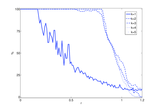
The main objective of the addition of a control term is to increase the size of the stability region around the central periodic orbit. This increase leads to decrease the number of escaping orbits, as we can see from the results presented in Fig. 2, where we plot in black the initial conditions on the square $(x_{1},x_{3})\in[-1,1]\times[-1,1]$, $x_{2}=x_{4}=0$, giving rise to orbits that do not escape up to $10^{5}$ iterations of the map. In particular, we consider in Fig. 2(a) the original uncontrolled map (1), and in Figs. 2(b) to 2(d), the $k$ order controlled map $T_{k}(F_{2})$ for $k=1$ to $k=5$ respectively. One can easily see that the region of non-escaping orbits for the original map is smaller than the one of the controlled maps. This observation can be quantified by considering initial conditions inside a circle centered at the origin of each panel of Fig. 2 (which represent the actual physical plane since the initial momenta are $x^{(0)}_{2}=x^{(k)}_{4}=0$) with radius $r^{2}={x^{(0)}_{1}}^{2}+{x^{(0)}_{3}}^{2}$, and evaluate the number of escaping and non-escaping orbits as a function of the circle radius for $T_{k}(F_{2})$ with $k=1$ up to $k=5$. Results reported in Fig. 3 support the previous claim, by clearly showing that controlled maps of orders $3$, $4$ and $5$ behave very similarly and lead to an increase of the non-escaping region. Let us note that the behavior of the controlled maps of orders $k=1$ (Fig. 2(b)) and $k=2$ (Fig. 2(c)) is somewhat misleading if it is not analyzed together with the information from the symplecticity defect (see Figs. 1(a) and (b) respectively). In fact, these maps are strongly dissipative and produce a strong shift of orbits towards the origin, preventing them from escaping. This dissipation effect is not physical, as it is not observed in real accelerators, and therefore we do not discuss further the $k=1$ and $k=2$ controlled maps.

Figure 2: Non-escaping regions of controlled map $T_{k}(F_{2})$ as a function of the truncation order $k$. $16000$ uniformly distributed initial conditions in the square $(x_{1},x_{3})\in[-1,1]\times[-1,1]$, $x^{(0)}_{2}=x^{(0)}_{4}=0$ are iterated up to $n=10^{5}$ using (a) the uncontrolled map (1) and (b)–(f) the $k=1$ to $k=5$ order controlled map $T_{k}(F_{2})$ (36), respectively. Initial conditions corresponding to non-escaping orbits up to $n=10^{5}$ are coloured in black, while escaping orbits are colored in white.

Figure 3: Percentages of non-escaping orbits for the controlled map $T_{k}(F_{2})$ (36) as a function of the distance from the origin in the physical space $(x_{1},x_{3})$. We iterate initial conditions in a circle of radius $r$ centred at the origin of plane $(x_{1},x_{3})$, with $x_{2}^{(0)}=x_{4}^{(0)}=0$, and compute the percentages of non-escaping orbits during $n=10^{5}$ iterations, for the controlled map $T_{k}(F_{2})$ with $k=1,2,3,4,5$, as a function of $r$.

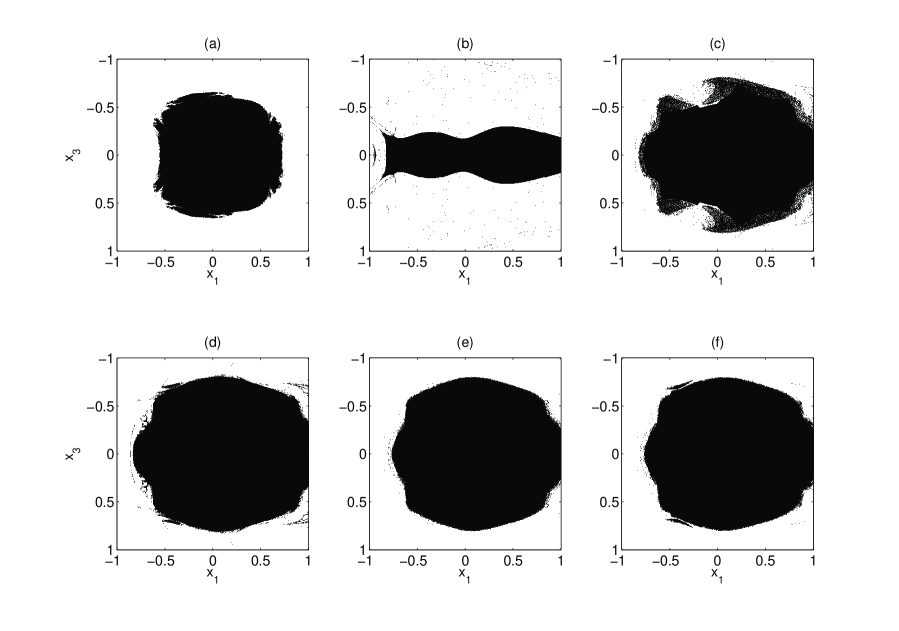
From the results of Figs. 2 and 3 we see that the addition of even the lower order ($k=3$) control term, having an acceptable symplecticity defect, increases drastically the size of the region of non-escaping orbits around the central periodic orbit. A further increase of the order of the control term results to less significant increment of this region, while the computational effort for constructing the controlled map increases considerably. In fact, $T_{1}(F_{2})$ contains around $100$ elementary terms, i.e. monomials in $x_{1}\dots x_{4}$, while this number is almost doubled for each order, so that $T_{5}(F_{2})$ contains around $2000$ terms. Also the CPU time needed to evolve the orbits increases with the order. For example, while the integration of one orbit using $T_{1}(F_{2})$ takes about $1.4$ times the CPU time needed to integrate the original map (1), the use of $T_{5}(F_{2})$ needs almost $21.5$ times more.

Thus we conclude that the $T_{4}(F_{2})$ controlled map, which can be considered quite accurately to be symplectic, is sufficient to get significant increment of the percentage of non-escaping orbits, without paying an extreme computational cost.

5 The SALI method

The Smaller Alignment Index (SALI) [10] has been proved to be an efficiently simple method to determine the regular or chaotic nature of orbits in conservative dynamical systems. Thanks to its properties, it has already been successfully distinguished between regular and chaotic motion both, in symplectic maps and Hamiltonian flows [11, 12, 13, 14, 15].

For the sake of completeness, let us briefly recall the definition of the SALI and its behavior for regular and chaotic orbits, restricting our attention to $2N$-dimensional symplectic maps. The interested reader can consult [10] for a more detailed description. To compute the SALI of a given orbit of such maps, one has to follow the time evolution of the orbit itself and also of two linearly independent unitary deviation vectors $\hat{v}_{1}^{(0)},\hat{v}_{2}^{(0)}$. The evolution of an orbit of a map $T$ is described by the discrete-time equations of the map

$$\vec{x}^{(n+1)}=T(\vec{x}^{(n)})\,,$$ (38)

where $\vec{x}^{(n)}=(x_{1}^{(n)},x_{2}^{(n)},...,x_{2N}^{(n)})^{\rm T}$, represents the orbit’s coordinates at the $n$-th iteration. The deviation vectors $\vec{v}_{1}^{(n)},\vec{v}_{2}^{(n)}$ at time $n$ are given by the tangent map

$$\vec{v}_{i}^{(n+1)}=A(\vec{x}^{(n)})\cdot\vec{v}_{i}^{(n)}\quad i=1,2\,,$$ (39)

where $A$ denotes the Jacobian matrix of map (38), evaluated at the points of the orbit under study. Then, according to [10] the SALI for the given orbit is defined as

$$\mbox{SALI}(n)=min\left\{\left\|\hat{v}_{1}^{(n)}+\hat{v}_{2}^{(n)}\right\|,\left\|\hat{v}_{1}^{(n)}-\hat{v}_{2}^{(n)}\right\|\right\}\,,$$ (40)

where $\|\cdot\|$ denotes the usual Euclidean norm and $\hat{v}_{i}=\frac{\vec{v}_{i}}{\|\vec{v}_{i}\|}$, $i=1,2$ are unitary normalised vectors.

In the case of chaotic orbits, the deviation vectors $\hat{v}_{1}$, $\hat{v}_{2}$ eventually become aligned in the direction defined by the maximal Lyapunov characteristic exponent (LCE), and SALI$(n)$ falls exponentially to zero. An analytical study of SALI’s behavior for chaotic orbits was carried out in [12] where it was shown that

$$\mbox{SALI}(n)\propto e^{-(\sigma_{1}-\sigma_{2})n},$$ (41)

with $\sigma_{1}$, $\sigma_{2}$ being the two largest LCEs.

On the other hand, in the case of regular motion the orbit lies on a torus and the vectors $\hat{v}_{1}$, $\hat{v}_{2}$ eventually fall on its tangent space, following a $n^{-1}$ time evolution, having in general different directions. This behavior is due to the fact that for regular orbits, the norm of a deviation vector increases linearly in time. Thus, the normalization procedure brings about a decrease of the magnitude of the coordinates perpendicular to the torus, at a rate proportional to $n^{-1}$, and so $\hat{v}_{1}$, $\hat{v}_{2}$ eventually fall on the tangent space of the torus. In this case, the SALI oscillates about non-zero values (for more details see [11]).

The simplicity of SALI’s definition, its completely different behavior for regular and chaotic orbits and its rapid convergence to zero in the case of chaotic motion are the main advantages that make SALI an ideal chaos detection tool. Recently a generalization of the SALI, the so-called Generalized Alignment Index (GALI) has been introduced [16, 17], which uses information of more than two deviation vectors from the reference orbit. Since the advantages of GALI over SALI become relevant in the case of multi-dimensional systems, in the present paper we apply the SALI method for the dynamical study of the 4D map (1).

6 Dynamics of the controlled map

As already mentioned, the goal of constructing the controlled map $T_{ctrl}=T\,e^{\{F\}}$ is to increase the percentage of regular orbits up to a given (large) number of iterations, or equivalently increase the size of the stability region around the nominal circular trajectory (i.e. the DA). Because the presence of chaotic regions can induce a large drift in the phase space, that eventually could lead to the escape of orbits, the achievement of a larger DA can be qualitatively inspected by checking via the SALI method the regular or chaotic nature of orbits in a neighborhood of the origin (see Fig. 4). We note that we define an orbit to be chaotic whenever SALI$(t)<10^{-8}$, and regular for the contrary.

Figure 4: Stability analysis in the $(x_{1},x_{3})$ plane. $16000$ uniformly distributed initial conditions in the square $(x_{1},x_{3})\in[-1,1]\times[-1,1]$, $x_{2}^{(0)}=x_{4}^{(0)}=0$ are integrated using the $T_{3}(F_{2})$ ((a) and (b)), and the $T_{4}(F_{2})$ controlled map ((c) and (d)), up to $n=10^{4}$ ((a) and (c)) and $n=10^{5}$ iterations ((b) and (d)). The gray scale represents the value of $\log_{10}$SALI for each orbit at the end of the integration time. The lighter the color the more stable is the orbit, while white color denotes that an orbit escaped before the total number of iterations was reached. The black circle indicate the initial condition of the orbit studied in Fig. 5.

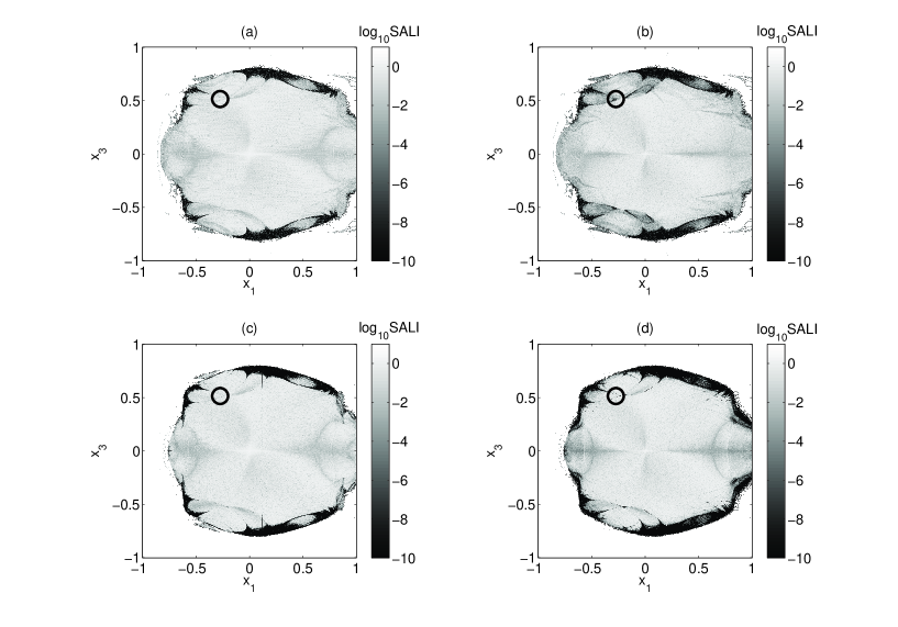
In Fig. 4 (which should be compared with Fig.5 of [6]) we observe a strong enlargement of the region of regular orbits. This region is characterized by large SALI values. In particular, for $10^{4}$ iterations of the $T_{4}(F_{2})$ map, $54\%$ of the considered orbits are regular, while for the uncontrolled map this percentage reduces to $33\%$. This improvement can be also confirmed by visual inspection of Fig. 2, where the regions of non-escaping orbits are shown for different orders of the controlled map (36).

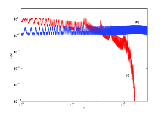
In Figs. 4(a) and (b) we see that there exist orbits of the $T_{3}(F_{2})$ map, which are characterized as regular up to $n=10^{4}$ iterations, while they show their chaotic character once they are iterated up to $n=10^{5}$. Such orbits correspond to the dark regions marked by a black circle in Fig. 4(b) (for comparison this circle is also plotted in all panels of Fig. 4). This discrepancy is absent for the $T_{4}(F_{2})$ map, which shows almost the same geometrical shape for the non-escaping region when we pass from $10^{4}$ to $10^{5}$ iterations. In order to better understand this behavior we followed the evolution of a single orbit with initial condition $\vec{x}^{(0)}=(-0.50,0,-0.65,0)^{T}$ –inside the black circle in Fig. 4– for both the $T_{3}(F_{2})$ and the $T_{4}(F_{2})$ controlled maps, computing the corresponding SALI values up to $2\times 10^{5}$ iterations. The results are reported in Fig. 5 and clearly show that the orbit behaves regularly up to $n\approx 10^{5}$ iterations of the $T_{3}(F_{2})$ map, since its SALI values are different from zero, but later on a sudden decrease of SALI to zero denotes the chaotic character of the orbit. This behavior clearly implies this is a slightly chaotic, sticky orbit, which remains close to a torus for long time intervals ($n\approx 10^{5}$), while later on it enters a chaotic region of the phase space. It is interesting to note that iterating the same initial condition by the $T_{4}(F_{2})$ map we get a regular behavior at least up to $n=2\times 10^{5}$.

Figure 5: (Color online) Dynamics of two orbits with the same initial conditions for the $3^{rd}$ and $4^{th}$ order controlled maps. Time evolution of the SALI for the orbit with initial conditions $\vec{x}^{(0)}=(-0.50,0,-0.65,0)^{T}$ (see Fig. 4), using the $T_{3}(F_{2})$ [(r) red curve] and the $T_{4}(F_{2})$ controlled map [(b) blue curve].

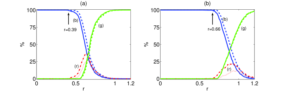
In order to provide additional numerical evidence of the effectiveness of the controlled map (36) in increasing the DA, we consider initial conditions inside a 4D sphere centered at the origin $x_{1}=x_{2}=x_{3}=x_{4}=0$ of the map, with radius, $r^{2}={{x_{1}^{(0)}}^{2}+{x_{2}^{(0)}}^{2}+{x_{3}^{(0)}}^{2}+{x_{4}^{(0)}}^{2}}$. We compute the number of regular, escaping and chaotic orbits as a function of the sphere radius. The corresponding results are reported in Fig. 6(b), while in Fig. 6(a) we reproduce Fig. 6 of [6] for comparison. From this figure we observe a strong increase of the DA, since the largest sphere containing $100\%$ regular orbits has a radius $r\approx 0.66$, while this radius was $r\approx 0.39$ for the original uncontrolled map. We also observe that increasing the total number of iterations from $10^{4}$ to $10^{5}$ (dashed and solid lines in Fig. 6 respectively) increases the percentage of chaotic orbits, but the radius of the 4D sphere containing only regular orbits does not change significantly.

Figure 6: (Color online) Dynamical aperture of the (a) original map (1) and (b) the $T_{4}(F_{2})$ controlled map (36). The percentages of regular [(b) blue curves], escaping [(g) green curves] and chaotic [(r) red curves] orbits after $n=10^{4}$ (dashed curves) and $n=10^{5}$ iterations (solid curves) for initial conditions in a 4D sphere centred at the origin $x_{1}=x_{2}=x_{3}=x_{4}=0$, as a function of the sphere radius $r$. Each point corresponds the average value over $5000$ initial conditions. The largest radius at which the percentage of regular orbits is still $100\%$, is marked by an arrow in each panel.

7 Conclusions

In this paper we considered a simple model of a ring particle accelerator with sextupole nonlinearity that can be described by a symplectic map. In the framework of Hamiltonian control theory, we were able to control the dynamics of the original system, by providing a suitable control map, resulting in a small “perturbation”of the initial map. This control map has been constructed with the aim of DA enlargement of the particle accelerator, and thus improving the beam’s life-time and the accelerator’s performance.

In particular, the theoretical framework we developed allows a $1$-parameter family of approximated controlled maps. We performed several numerical simulations in order to choose “the best”approximated controlled map $T_{k}(F_{2})$ (36), taking into account the complexity of the map, i.e. the number of terms by which it is composed, the CPU time needed to perform the numerical iteration of orbits, and the accuracy of the results in terms of the symplectic character of the map. We find that the $4^{th}$ order controlled map $T_{4}(F_{2})$ is an optimal choice for the controlled system.

Using this controlled map we succeeded in achieving our initially set goal, since the $T_{4}(F_{2})$ map exhibits a DA with a radius more than $1.7$ times larger than the one for the original map (see Fig. 6).

Appendix A Computation of the control term.

The aim of this section is to introduce further details for the construction of the control term and of the controlled map, and to provide explicit formulas for the interested reader.

A.1 Notations

Let us first introduce some notations and recall some useful relations.

• Lie brackets and operators. Let $\mathcal{X}$ be the vector space of $C^{\infty}$ real or complex functions of $2N$ variables $(p,q)$. For any $F,\,G\,\in\mathcal{X}$, the Lie bracket is given by

  $$\{F,G\}:=\sum_{i=1}^{N}\left[\partial_{p_{i}}F\partial_{q_{i}}G-\partial_{q_{i}}F\partial_{p_{i}}G\right]\,,$$ (42)

  where $\partial_{x_{i}}f\equiv\frac{\partial f}{\partial x_{i}}$ denotes the partial derivative with respect to the variable $x_{i}$.

  Using the above definition, we can define a linear operator, induced by an element $F$ of $\mathcal{X}$, acting on $\mathcal{X}$

  $$\begin{array}[]{rccl}\{F\}:&\mathcal{X}&\rightarrow&\mathcal{X}\\ &G&\mapsto&\{F\}G:=\{F,G\}\end{array}$$ (43)

  This operator is linear, antisymmetric and verifies the Jacobi identity

  $$\forall F,G\in\mathcal{X}\quad\{\{F\}G\}=\{F\}\{G\}-\{G\}\{F\}$$ (44)

• Exponential. We define the exponential of such an operator $\{F\}$, by

  $$e^{\{F\}}:=\sum_{k=0}^{\infty}\frac{\{F\}^{k}}{k!}\,,$$ (45)

  which is also an operator acting on $\mathcal{X}$. The power of an operator is the composition : $\{F\}^{k}G=\{F\}^{k-1}\left(\{F\}G\right)$.

  We observe that in the case of the Hamiltonian function $H$, the exponential provides the flow, namely $e^{\{H\}}x_{0}=x(t)$, of the Hamilton equations

  $$\begin{cases}\dot{p}&=-\partial_{q}H\\ \dot{q}&=\partial_{p}H\,.\end{cases}$$ (46)

• Vector Field. The action of the above defined operators, can be extended to vector fields “component by component”

  $$\forall\,F,G,H\in\mathcal{X}\quad\{F\}\left(\begin{array}[]{c}G\\ H\end{array}\right):=\left(\begin{array}[]{c}\{F\}G\\ \{F\}H\end{array}\right).$$ (47)

A.2 Mappings as time-$1$ flows.

We show now that map (1) can be seen as the time-$1$ flow of a given Hamiltonian system. More precisely we show that

$$T\left(\begin{array}[]{c}x_{1}\\ x_{2}\\ x_{3}\\ x_{4}\end{array}\right) = \left(\begin{array}[]{cccc}\cos(\omega_{1})&-\sin(\omega_{1})&0&0\\ \sin(\omega_{1})&\cos(\omega_{1})&0&0\\ 0&0&\cos(\omega_{2})&-\sin(\omega_{2})\\ 0&0&\sin(\omega_{2})&\cos(\omega_{2})\end{array}\right)\left(\begin{array}[]{c}x_{1}\\ x_{2}+x_{1}^{2}-x_{3}^{2}\\ x_{3}\\ x_{4}-2x_{1}x_{3}\end{array}\right)$$ (60)

$$= e^{\{H\}}e^{\{V\}}\left(\begin{array}[]{c}x_{1}\\ x_{2}\\ x_{3}\\ x_{4}\end{array}\right)$$ (65)

where

$$H(x_{1},x_{2},x_{3},x_{4})=-\omega_{1}\frac{x_{1}^{2}+x_{2}^{2}}{2}-\omega_{2}\frac{x_{3}^{2}+x_{4}^{2}}{2}$$ (66)

and

$$V(x_{1},x_{2},x_{3},x_{4})=-\frac{x_{1}^{3}}{3}+x_{1}x_{3}^{2}\,.$$ (67)

Let us observe that $H$ is the sum of two non-interacting harmonic oscillators with frequencies $\omega_{1}$ and $\omega_{2}$, hence its dynamics is explicitly given by

$$\begin{cases}x_{1}(t)&=A\cos(\omega_{1}t)-B\sin(\omega_{1}t)\\ x_{2}(t)&=B\cos(\omega_{1}t)+A\sin(\omega_{1}t)\\ x_{3}(t)&=C\cos(\omega_{2}t)-D\sin(\omega_{2}t)\\ x_{4}(t)&=D\cos(\omega_{2}t)+C\sin(\omega_{2}t)\,.\end{cases}$$ (68)

By definition $\vec{y}=e^{\{H\}}\vec{x}$ is the solution at time $1$ with initial condition $\vec{x}=(x_{1},x_{2},x_{3},x_{4})^{T}$, hence we obtain

$$\begin{cases}y_{1}&=\cos(\omega_{1})x_{1}-\sin(\omega_{1})x_{2}\\ y_{2}&=\sin(\omega_{1})x_{1}+\cos(\omega_{1})x_{2}\\ y_{3}&=\cos(\omega_{2})x_{3}-\sin(\omega_{2})x_{4}\\ y_{4}&=\sin(\omega_{2})x_{3}+\cos(\omega_{2})x_{4}\,,\end{cases}$$ (69)

that is

$$e^{\{H\}}\left(\begin{array}[]{c}x_{1}\\ x_{2}\\ x_{3}\\ x_{4}\end{array}\right)=\left(\begin{array}[]{cccc}\cos(\omega_{1})&-\sin(\omega_{1})&0&0\\ \sin(\omega_{1})&\cos(\omega_{1})&0&0\\ 0&0&\cos(\omega_{2})&-\sin(\omega_{2})\\ 0&0&\sin(\omega_{2})&\cos(\omega_{2})\end{array}\right)\left(\begin{array}[]{c}x_{1}\\ x_{2}\\ x_{3}\\ x_{4}\end{array}\right)\,.$$ (70)

From (67) and the definition (43) we easily get

$$\{V\} := \partial_{x_{2}}V\partial_{x_{1}}-\partial_{x_{1}}V\partial_{x_{2}}+\partial_{x_{4}}V\partial_{x_{3}}-\partial_{x_{3}}V\partial_{x_{4}}$$

$$= (x_{1}^{2}-x_{3}^{2})\partial_{x_{2}}-2x_{1}x_{3}\partial_{x_{4}}.$$

This means that once applied to a vector $\vec{x}$ only the second and fourth components of $\{V\}\vec{x}$ will be non-zero and moreover they only depend on the first and third components of $\vec{x}$, hence $\{V\}^{2}\vec{x}=\vec{0}$. We can thus conclude that $\forall\,k\geq 2$ and $\forall\vec{x}\in\mathbb{R}^{4}$, we get $\{V\}^{k}\vec{x}=\vec{0}$. Finally using the definition (45) we obtain

$$e^{\{V\}}\vec{x}=\sum_{k=0}^{\infty}\frac{\{V\}^{k}}{k!}\vec{x}=I\vec{x}+\{V\}\vec{x}=\left(\begin{array}[]{c}x_{1}\\ x_{2}+x_{1}^{2}-x_{3}^{2}\\ x_{3}\\ x_{4}-2x_{1}x_{3}\end{array}\right)$$ (72)

A.3 Computation of the generator $F$ under the assumption $\mathcal{R}V\equiv 0$.

Let us recall that the composition of maps expressed by exponential defines the warped addition

$$e^{\{A\}}e^{\{B\}}:=e^{\{A\}\oplus\{B\}}\,,$$ (73)

whose first terms are

$$\{A\}\oplus\{B\}=\{A\}+\{B\}+\frac{1}{2}(\{A\}\{B\}-\{B\}\{A\})+\dots$$ (74)

Using the warped addition with equation (13) of Theorem 3.1, we obtain

$$e^{\{F\}}=e^{-\{V\}}e^{\{(\mathcal{N}-\mathcal{G})V\}}e^{\{\mathcal{R}V\}}e^{\{\mathcal{\mathcal{G}V}\}}=e^{-\{V\}\oplus\{(\mathcal{N}-\mathcal{G})V\}\oplus\{\mathcal{R}V\}\oplus\{\mathcal{\mathcal{G}V}\}}\,,$$ (75)

and thus

$$\{F\} = -\{V\}\oplus\{(\mathcal{N}-\mathcal{G})V\}\oplus\{\mathcal{R}V\}\oplus\{\mathcal{\mathcal{G}V}\}=-\{V\}\oplus\{(1-\mathcal{G})V\}\oplus\{\mathcal{G}V\}+o(V^{2})$$ (76)

$$= \left[\frac{1}{2}\underbrace{\left(\{V\}\{\mathcal{G}V\}-\{\mathcal{G}V\}\{V\}\right)}_{\stackrel{{\scriptstyle(\ref{jacobi})}}{{=}}\{\{V\}\mathcal{G}V\}}-\{\mathcal{G}V\}\right]\oplus\{\mathcal{G}V\}+o(V^{2})$$

$$= \frac{1}{2}\{\{V\}\mathcal{G}V\}+\frac{1}{4}\underbrace{\{\{\{V\}\mathcal{G}V\}\mathcal{G}V\}}_{=o(V^{2})}+o(V^{2})=\frac{1}{2}\{\{V\}\mathcal{G}V\}+o(V^{2})\,,$$

where we explicitly used the assumption $\mathcal{R}V=0$ to remove the third term on the the right hand side on the first equation and hence to write $\mathcal{N}V=V$. We are thus able to define the non-resonant control term, up to order $V^{2}$, to be

$$F_{2}=\frac{1}{2}\{V\}\mathcal{G}V=\frac{1}{2}\{V,\mathcal{G}V\}\,.$$ (77)

A.4 The operator $\mathcal{G}$

To get the explicit formula for $F_{2}$ we need to compute the expression of $\mathcal{G}$. ¿From definition (9) the operator $\mathcal{G}$ should satisfy

$$\mathcal{G}\left(1-e^{-\{H\}}\right)\mathcal{G}=\mathcal{G}\,.$$ (78)

To construct it, it will be more convenient to use complex variables

$$\zeta_{1}=x_{2}+ix_{1}\quad\text{and}\quad\zeta_{2}=x_{4}+ix_{3}\,.$$ (79)

Then the function $H$ becomes

$$H(\zeta_{1},\zeta_{2})=-\frac{\omega_{1}}{2}\zeta_{1}\bar{\zeta}_{1}-\frac{\omega_{2}}{2}\zeta_{2}\bar{\zeta}_{2}\,,$$ (80)

and using

$$\frac{\partial}{\partial x_{1}} = \frac{\partial\zeta_{1}}{\partial x_{1}}\frac{\partial}{\partial\zeta_{1}}+\frac{\partial\bar{\zeta}_{1}}{\partial x_{1}}\frac{\partial}{\partial\bar{\zeta}_{1}}=i\frac{\partial}{\partial\zeta_{1}}-i\frac{\partial}{\partial\bar{\zeta}_{1}}$$ (81)

$$\frac{\partial}{\partial x_{2}} = \frac{\partial\zeta_{1}}{\partial x_{2}}\frac{\partial}{\partial\zeta_{1}}+\frac{\partial\bar{\zeta}_{1}}{\partial x_{2}}\frac{\partial}{\partial\bar{\zeta}_{1}}=\frac{\partial}{\partial\zeta_{1}}+\frac{\partial}{\partial\bar{\zeta}_{1}}$$ (82)

for $(x_{1},x_{2})$, the operator $\{H\}$ becomes

$$\partial_{x_{2}}H\partial_{x_{1}}-\partial_{x_{1}}H\partial_{x_{2}}=2i\left(\partial_{\zeta_{1}}H\partial_{\bar{\zeta}_{1}}-\partial_{\bar{\zeta}_{1}}H\partial_{\zeta_{1}}\right)=i\omega_{1}\left(\bar{\zeta}_{1}\partial_{\bar{\zeta}_{1}}-\zeta_{1}\partial_{\zeta_{1}}\right)\,,$$ (83)

with a similar expression holding for $(x_{3},x_{4})$. Hence for any $\vec{n}=(n_{1},n_{2})\in\mathbb{N}^{2}$ and $\vec{m}=(m_{1},m_{2})\in\mathbb{N}^{2}$ we obtain

$$\{H\}{\zeta}^{\vec{n}}\bar{{\zeta}}^{\vec{m}}=i\left(\omega_{1}m_{1}-\omega_{1}n_{1}+\omega_{2}m_{2}-\omega_{2}n_{2}\right){\zeta}^{\vec{n}}\bar{{\zeta}}^{\vec{m}}=i\vec{\omega}\cdot(\vec{m}-\vec{n}){\zeta}^{\vec{n}}\bar{{\zeta}}^{\vec{m}}\,,$$ (84)

where we introduced the vector $\vec{\omega}=(\omega_{1},\omega_{2})$ and we used the compact notation ${\zeta}^{\vec{n}}=\zeta_{1}^{n_{1}}\zeta_{2}^{n_{2}}$, for the complex vector ${\zeta}=(\zeta_{1},\zeta_{2})$.

We note that from the knowledge of the operators’ action on such monomials $\zeta^{\vec{n}}\bar{\zeta}^{\vec{m}}$, we can reconstruct the operator action on any regular function. The operators are linear and they will be applied on polynomials in the $\vec{x}$ variable, which are nothing more than polynomials in the complex variables.

Let us now compute the time-$1$ flow of $\{H\}$ by using complex variables. Starting from  (84) and then proceeding by induction, we can easily prove that for all $k\in\mathbb{N}$

$$\{H\}^{k}\zeta^{\vec{n}}\bar{\zeta}^{\vec{m}}=\left(i\vec{\omega}\cdot(\vec{m}-\vec{n})\right)^{k}\zeta^{\vec{n}}\bar{\zeta}^{\vec{m}}\,,$$ (85)

and finally

$$e^{\{H\}}{\zeta}^{\vec{n}}\bar{\zeta}^{\vec{m}}=\sum_{k=0}^{\infty}\frac{\left(i\vec{\omega}\cdot(\vec{m}-\vec{n})\right)^{k}}{k!}{\zeta}^{\vec{n}}\bar{{\zeta}}^{\vec{m}}=e^{i\vec{\omega}\cdot(\vec{m}-\vec{n})}{\zeta}^{\vec{n}}\bar{\zeta}^{\vec{m}}.$$ (86)

Similarly $e^{-\{H\}}{\zeta}^{\vec{n}}\bar{{\zeta}}^{\vec{m}}=e^{-i\vec{\omega}\cdot(\vec{m}-\vec{n})}{\zeta}^{\vec{n}}\bar{{\zeta}}^{\vec{m}}$.

Assuming a non-resonance condition

$$\vec{\omega}\cdot(\vec{m}-\vec{n})\neq 2k\pi\quad\forall\vec{n}\neq\vec{m}\in\mathbb{N}^{2}\setminus\{0\}\quad\text{and}\quad\forall k\in\mathbb{Z}\,,$$ (87)

a possible choice for the operator $\mathcal{G}$ is the following

$$\mathcal{G}{\zeta}^{\vec{n}}\bar{{\zeta}}^{\vec{m}}:=\frac{1}{1-e^{-i\vec{\omega}\cdot(\vec{m}-\vec{n})}}\mathcal{N}{\zeta}^{\vec{n}}\bar{{\zeta}}^{\vec{m}}$$ (88)

with

$$\mathcal{N}{\zeta}^{\vec{n}}\bar{{\zeta}}^{\vec{m}}=\begin{cases}{\zeta}^{\vec{n}}\bar{{\zeta}}^{\vec{m}}&\text{if $\vec{\omega}\cdot(\vec{m}-\vec{n})\neq 2\pi k$}\\ 0&\text{otherwise}\end{cases}\,.$$ (89)

It is easy to check that the operator $\mathcal{G}$ defined by (88) verifies (78). In order to do so we introduce the compact notation

$$Z_{n,m}:={\zeta}^{\vec{n}}\bar{{\zeta}}^{\vec{m}}\quad\text{and}\quad\square_{n,m}:=e^{-i\vec{\omega}\cdot(\vec{m}-\vec{n})}\,.$$ (90)

Developing the left hand side of (78) and using the linearity of all operators, we get

$$\mathcal{G}\left(1-e^{-\{H\}}\right)\mathcal{G}Z_{n,m} = \left(\mathcal{G}-\mathcal{G}e^{-\{H\}}\right)\frac{1}{1-\square_{n,m}}Z_{n,m}$$ (91)

$$= \frac{1}{1-\square_{n,m}}\mathcal{G}Z_{n,m}-\frac{1}{1-\square_{n,m}}\mathcal{G}e^{-\{H\}}Z_{n,m}$$ (92)

$$= \frac{1}{(1-\square_{n,m})^{2}}Z_{n,m}-\frac{1}{1-\square_{n,m}}\mathcal{G}(\square_{n,m}Z_{n,m})$$ (93)

$$= \frac{1}{(1-\square_{n,m})^{2}}Z_{n,m}-\frac{\square_{n,m}}{(1-\square_{n,m})^{2}}Z_{n,m}$$ (94)

$$= \frac{1}{1-\square_{n,m}}Z_{n,m}=\mathcal{G}Z_{n,m}\,.$$ (95)

A.5 Expression of the control term $F_{2}$

The function $F_{2}$ is defined by (77), where $V$ is a known function. The term $\mathcal{G}V$ will be computed starting from the previously obtained expression of $\mathcal{G}$. To construct $F_{2}$ we first have to express $V$ in the complex variables (79):

$$V(\zeta_{1},\zeta_{2})=-\frac{1}{24}i\zeta_{1}^{3}+\frac{1}{8}i\bar{\zeta}_{1}\zeta_{1}^{2}-\frac{1}{8}i\bar{\zeta}_{1}^{2}\zeta_{1}+\frac{1}{24}i\bar{\zeta}_{1}^{3}+\frac{1}{8}i\zeta_{1}\zeta_{2}^{2}-\frac{1}{4}i\zeta_{1}\zeta_{2}\bar{\zeta}_{2}$$

$$+\frac{1}{8}i\zeta_{1}\bar{\zeta}_{2}^{2}-\frac{1}{8}i\bar{\zeta}_{1}\zeta_{2}^{2}+\frac{1}{4}i\bar{\zeta}_{1}\bar{\zeta}_{2}\zeta_{2}-\frac{1}{8}i\bar{\zeta}_{1}\bar{\zeta}_{2}^{2}\,.$$ (96)

By the linearity of the operator, and by using (88), we easily compute $\mathcal{G}V$. In particular we apply $\mathcal{G}$ to each term of (96). Then using the inverse change of coordinates

$$x_{1}=\frac{1}{2}i(\bar{\zeta}_{1}-\zeta_{1})\quad\text{and}\quad x_{2}=\frac{1}{2}(\zeta_{1}+\bar{\zeta}_{1})\,$$ (97)

(similar expressions hold for $(x_{3},x_{4})$ and $(\zeta_{2},\bar{\zeta}_{2})$), we can go back to the original variables $\vec{x}$. The obtained expression after some algebraic simplifications is

$$\mathcal{G}V = -1/6\,\csc\left(3/2\,\omega_{1}\right)\left[x_{2}\,\cos\left(1/2\,\omega_{1}\right)+x_{1}\,\sin\left(1/2\,\omega_{1}\right)\right]\left[{x_{1}}^{2}-3\,{x_{3}}^{2}+{x_{2}}^{2}\right.$$ (98)

$$\left.+\left(2\,{x_{1}}^{2}-6\,{x_{3}}^{2}+{x_{2}}^{2}\right)\cos\left(\omega_{1}\right)-x_{1}\,x_{2}\,\sin\left(\omega_{1}\right)\right]$$

$$+1/4\,{\frac{\sin\left(\omega_{2}\right)}{\cos\left(\omega_{1}-\omega_{2}\right)-\cos\left(\omega_{2}\right)}}$$

$$-1/4\,{\frac{\left(-x_{2}\,{x_{4}}^{2}+x_{2}\,{x_{3}}^{2}+2\,x_{1}\,x_{4}\,x_{3}\right)\sin\left(\omega_{2}\right)}{\cos\left(\omega_{2}\right)-\cos\left(\omega_{1}+\omega_{2}\right)}}$$

Then the explicit expression of the control term $F_{2}$ is

$$F_{2} = 1/2(x_{1}^{2}-x_{3}^{2})\Bigg{(}-1/6\csc(3/2\omega_{1})\cos(1/2\omega_{1})(x_{1}^{2}-3x_{3}^{2}+x_{2}^{2}$$ (99)

$$+(2x_{1}^{2}-6x_{3}^{2}+x_{2}^{2})\cos(\omega_{1})-x_{1}x_{2}\sin(\omega_{1}))$$

$$-1/6\csc(3/2\omega_{1})\Big{(}x_{2}\cos(1/2\omega_{1})+x_{1}\sin(1/2\omega_{1})\Big{)}(2x_{2}+2x_{2}\cos(\omega_{1})-x_{1}\sin(\omega_{1}))$$

$$-1/4{\frac{(x_{3}^{2}-x_{4}^{2})\sin(\omega_{2})}{\cos(\omega_{2})-\cos(\omega_{1}+\omega_{2})}}\Bigg{)}+1/4{\frac{x_{1}x_{3}(2x_{1}x_{3}-2x_{2}x_{4})\sin(\omega_{2})}{\cos(\omega_{2})-\cos(\omega_{1}+\omega_{2})}}.$$

References

- [1] Giovanozzi M, Scandale W and Todesco E 1997 Part. Accel. 56 195
- [2] Bountis T and Tompaidis S 1991 G. Turchetti, W. Scandale (Eds.), World Scientific, Singapore 112
- [3] Bountis T and Kollmann M 1994 Physica D 71 122
- [4] Vrahatis M N Bountis T and Kollmann M 1996 Int. J. Bifur. and Chaos 6 (8) 1425
- [5] Vrahatis M N Isliker H and Bountis T 1997 Int. J. Bifur. and Chaos 7 (12) 2707
- [6] Bountis T and Skokos Ch 2006 Nucl. Instr. Meth. Phys. Res. - Sect. A 561 173
- [7] Vittot M 2004 J. Phys. A: Math. Gen. 37 6337
- [8] Chandre C, Vittot M, Elskens Y, Ciraolo G and Pettini M 2005 Physica D 208 131
- [9] Bourbaki N 1972 Eléments de Mathématiques: Groupes et Algèbres de Lie (Hermann Ed. Paris)
- [10] Skokos Ch 2001 J. Phys. A 34 10029
- [11] Skokos Ch, Antonopoulos Ch, Bountis T and Vrahatis M N 2003 Prog. Theor. Phys. Supp. 150 439
- [12] Skokos Ch, Antonopoulos Ch, Bountis T C and Vrahatis M N 2004 J. Phys. A 37 6269
- [13] Széll A, Érdi B, Sándor Zs and Steves B 2004 MNRAS 347 380
- [14] Panagopoulos P, Bountis T C and Skokos Ch 2004 J. Vib. & Acoust. 126 520
- [15] Manos T, Athanassoula E 2005 Proceedings of Semaine de l’ Astrophysique Française Journées de la SF2A eds F Caloli, T Contini, J M Hameury and L Pagani (EDP-Science Conference Series) p 631
- [16] Skokos Ch, Bountis T and Antonopoulos Ch 2007 J. Phys. D 231 30
- [17] Skokos Ch, Bountis T and Antonopoulos Ch Eur. Phys. J. Sp. T. 165 5