A magnetic field evolution scenario for brown dwarfs
and giant planets

Very little is known about magnetic fields of extrasolar planets and brown dwarfs. We use the energy flux scaling law presented by Christensen et al. (2009) to calculate the evolution of average magnetic fields in extrasolar planets and brown dwarfs under the assumption of fast rotation, which is probably the case for most of them. We find that massive brown dwarfs of about 70 M_Jup can have fields of a few kilo-Gauss during the first few hundred Million years. These fields can grow by a factor of two before they weaken after deuterium burning has stopped. Brown dwarfs with weak deuterium burning and extrasolar giant planets start with magnetic fields between $\sim$100 G and $\sim$1 kG at the age of a few Myr, depending on their mass. Their magnetic field weakens steadily until after 10 Gyr it has shrunk by about a factor of 10. We use observed X-ray luminosities to estimate the age of the known extrasolar giant planets that are more massive than 0.3 M_Jup and closer than 20 pc. Taking into account the age estimate, and assuming sun-like wind-properties and radio emission processes similar to those at Jupiter, we calculate their radio flux and its frequency. The highest radio flux we predict comes out as 700 mJy at a frequency around 150 MHz for $\tau$ Boo b, but the flux is below 60 mJy for the rest. Most planets are expected to emit radiation between a few Mhz and up to 100 MHz, well above the ionospheric cutoff frequency.

1 Introduction

The discovery of hundreds of extrasolar planets during the last two decades has enabled us to investigate the physical properties of these objects, and to compare them to the known planets of our own solar system. The discoveries of brown dwarfs, on the other hand, have opened our view for this interesting class of objects placed between stars and planets and sharing physical properties with both groups. Particularly interesting questions are whether planets, brown dwarfs, and stars share the same physical principles with regard to their magnetic dynamos, and what typical field strengths must be expected at objects for which a positive field detection is missing so far (brown dwarfs and exoplanets).

Radioemissions from magnetized planets result from the interaction of their magnetospheres with the stellar wind. This accelerates electrons to several keV, which emit radio waves at the local cyclotron frequency (e.g., Zarka, 1992, 1998; Farrell et al., 1999; Zarka, 2007). A similar mechanism, the electron cyclotron maser, was identified as the dominant source of radio emission for a number of very-low mass stars and brown dwarfs (Hallinan et al., 2008). Radio emissions from extrasolar planets are particularly interesting because they can outshine the radio emission from a quiet host star (e.g., Farrell et al., 1999; Grießmeier et al., 2005), and may therefore be utilized to discover extrasolar planets. So far, none of the searches for radio emission from extrasolar planets could present a positive detection. This is not too surprising because currently available facilities are hardly sensitive enough to observe the expected weak radio flux.

Both the frequency and the total radio flux depend critically on the magnetic field strength of the planet, the latter primarily because it controls the cross section of the magnetosphere interacting with the stellar wind. In addition, the energy flux of the wind, which depends on the planet’s distance from the host star and on stellar activity, plays an important role for the total radio flux. The spectrum of the radio emission is expected to show a sharp cutoff at the electron cyclotron frequency corresponding to the maximum magnetic field strength close to the planetary surface. Future observations of the radio spectrum of extrasolar planets can therefore constrain the field strength rather reliably.

Usually, one assumes that radio emission can be generated at extrasolar planets in much the same way as they are generated at Jupiter. Recent estimates of radio fluxes from known extrasolar planets were presented by Farrell et al., (1999), Lazio et al., (2004), Stevens, (2005), Grießmeier et al., 2007a , and Jardine & Cameron, (2008). One of the large uncertainties in the prediction of radio emission is the magnetic moment of extrasolar planets. Grießmeier et al., (2004) discussed the different magnetic moment scaling laws that were available at that time and applied them to estimate the field of extrasolar planets. Christensen & Aubert, (2006) derived a magnetic field scaling relation for planets based on dynamos simulations that cover a broad parameter range. Recently, Christensen et al., (2009) generalized the scaling law and showed that its predictions agree with observations for a wide class of rapidly rotating objects, from Earth and Jupiter to low-mass main sequence (spectral types K and M) and T Tauri stars (see also Christensen, 2009). Here, we revisit the question of magnetic field strength at brown dwarfs and giant planets and the estimate for the radio flux from extrasolar planets, using this scaling law, which we believe to be on more solid grounds both theoretically and observationally than previously suggested scaling laws.

2 Magnetic flux estimate

Here we use this scaling law in the form given by Reiners et al., 2009b , who expressed the magnetic field strength in terms of mass $M$, luminosity $L$ and radius $R$ (all normalized with solar values):

$$B_{\rm dyn}=4.8\times\left(\frac{ML^{2}}{R^{7}}\right)^{1/6}\rm{[kG]},$$ (1)

where $B_{\rm dyn}$ is the mean magnetic field strength at the surface of the dynamo.

In its original form (Christensen et al., 2009), the scaling relation connects the strength of the magnetic field to the one-third power of the energy flux (luminosity divided by surface area). It is independent of the rotation rate, provided the latter is sufficiently high. A weak 1/6-power dependence on the mean density and a factor describing the thermodynamic efficiency of magnetic field generation also enter into the scaling law. The latter factor is found to be close to one for a large class of objects (Christensen et al., 2009), and this value has been used in Eq. 1. Aside from this assumption, the value of the numerical prefactor in this equations is only based on the results of dynamo simulations.

For massive brown dwarfs and stars the top of the dynamo is close to or at the surface of the object and the value of $B_{\rm dyn}$ is directly relevant for observations that relate to the magnetic field strength. In giant planets, with $M<13M_{\rm J}$ (13 Jupiter masses), the surface of the dynamo region is at some depth, for example in Jupiter at approximately 83 % of the planet’s radius and the field at the surface is somewhat smaller (Christensen et al., 2009). Higher multipole components, which are assumed to make up half of $B_{\rm dyn}$, drop off rapidly with radius and are neglected for simplicity. The radius of objects with masses between 0.3 and 70 $M_{\rm J}$ is nearly constant within $\pm$ 20% of one Jupiter radius for ages larger than 200 Myr (Burrows et al., 2001). In this case the depth to the top of the dynamo, at the pressure of metallization of hydrogen in a H-He planet, is approximately inversely proportional to the mass. We relate the dipole field strength at the equator of a giant planet, $B_{\rm dip}^{\rm eq}$, to the overall field strength at the top of the dynamo, $B_{\rm dyn}$, by

$$B_{\rm dip}^{\rm eq}=\frac{B_{dyn}}{2\sqrt{2}}\left(1-\frac{0.17}{M/{\rm M}_{\rm J}}\right)^{3}.$$ (2)

The factor $2\sqrt{2}$ in the denominator results from the assumption that at the dynamo surface the dipole field strength is half of the rms field strength and from the fact that the equatorial dipole field is $1/\sqrt{2}$ of the rms dipole field.

To estimate the field strength of substellar objects, we employ in Eq. 1 radii and luminosities from the evolutionary tracks calculated by Burrows et al., (1993, 1997) for substellar objects. Our model predicts a magnetic field of 9 G for an object of one $M_{\rm J}$ at an age of 4.5 Gyr. This value agrees well with the polar dipole field strength of Jupiter, which is 8.4 G (e.g., Connerney, 1993).

2.1 Rotation of the planets

We implicitly assume that the objects are rotating above a critical rotation velocity, so that our scaling law can be applied. This seems to be the case in most of the solar-system giant planets (Christensen, 2009, Section 4) and in brown dwarfs (Reiners & Basri, 2008). Giant planets with semimajor axes less than about 0.1 – 0.2 AU are expected to be slowed down to synchronous rotation by tidal braking on time scales of less than 1 Gyr (Seager & Hui, 2002). However, for planets that are very close to their host star the synchronous rotation rate may still lie above the critical limit for our scaling law to apply; the value of the latter is somewhat uncertain. M-dwarfs with rotation periods up to at least 4 days are generally found to fall into the magnetically saturated regime (Reiners et al., 2009a ) for which our scaling law applies. We emphasize that our results can be considered as upper limits and would be lower if the objects for some reason would rotate substantially slower.

3 Radio flux calculation

We estimate the magnetospheric radio flux from extrasolar giant planets following the work of Stevens, (2005). This means we assume that the input power into the magnetosphere is proportional to the total kinetic energy flux of the stellar wind. Grießmeier et al., 2007a discussed different mechanisms depending on the source of available energy. They also calculate radio emission for the case where the input power is provided by magnetic energy of the interplanetary field, for unipolar magnetic interaction, and for stellar flares. In general, stellar activity of planet host stars is relatively weak so that we concentrate on the kinetic energy flux as source for the power input.

3.1 Radio flux scaling law

In order to calculate the radio flux of a giant extrasolar planet at the location of the Earth, we relate it to the radio flux of Jupiter using Equation (14) from (Stevens, 2005) neglecting the dependence on the wind-velocity (see below):

$$P\propto\frac{1}{d^{2}}\left(\frac{\dot{M}_{\star}M_{\rm dip}}{a^{2}}\right)^{2/3},$$ (3)

with $P$ the radio flux, $d$ the distance to the system, $\dot{M}_{\star}$ the stellar mass-loss rate, $M_{\rm dip}$ the dipole moment of the planet, and $a$ the star-planet distance. The dipole moment is

$$M_{\rm dip}=B_{\rm dip}^{\rm eq}R^{3},$$ (4)

with $R$ the planetary radius. We assume Jupiter-like values for the stellar wind velocity, $V_{W}=400$ km s^-1. As discussed in Stevens, (2005), the latter may be an overestimate in particular for close-in planets, because wind velocities are lower closer to the star. We also note that young stars have higher mass-loss ratios (Wood et al., 2005), but this does not necessarily affect the wind velocities (see also Wood et al., 2002, who assume a fixed stellar wind velocity). Nevertheless, our uncertainties in the wind velocities are probably on the order of a factor of two, which means about a factor of $\sim 3$ (0.5 dex) uncertainty for individual stars. We refer to Stevens, (2005) for further details. In our approximation, for a given semi-major axis, mass-loss rate and distance, the radio flux is only a function of the magnetic moment or the average magnetic field.

The electron cyclotron frequency near the surface in the polar region is $f_{\rm ce}[{\rm MHz}]=2.8B_{\rm dip}^{\rm pol}[{\rm G}]$, where $B_{\rm dip}^{\rm pol}=2B_{\rm dip}^{\rm eq}$ is the polar dipole field strength. For Jupiter it corresponds roughly to the cutoff frequency observed in the radio emission spectrum (see Zarka, 1992). The bulk of Jupiter’s radio flux occurs in roughly the frequency range from 0.1 $f_{\rm ce}$ to the cutoff frequency.

3.2 Parameter estimates for known host stars

3.2.1 Mass-loss rate

To calculate the mass-loss rate that is required in Eq. (3) for host stars of known extrasolar giant planets (EGPs), we parameterize the stellar mass-loss rates using the results from Wood et al., (2005) and use X-ray luminosities taken from the NEXXUS database (Schmitt & Liefke, 2004) in analogy with Stevens, (2005) but with the updated parameters from Wood et al., (2005)

$$\frac{\dot{M}_{\star}}{{\rm\dot{M}}_{\odot}}=\left(\frac{R_{\star}}{{\rm R}_{\odot}}\right)^{2}\left(\frac{F_{X}}{{\rm F}_{X,\odot}}\right)^{1.34}.$$ (5)

With $F_{X}=L_{X}/(4\pi R^{2})$, we get the mass-loss rate as a function of X-ray luminosity times $(R_{\star}/{\rm R}_{\odot})^{-0.68}$. The latter factor introduces an error on the order of $\sim 10$ % if the radius differs from the solar radius by 20 %. A radius offset of 50 % (i.e. for example between 0.6 and 0.9 R_⊙, which is the difference in radius between a G-type star and an early-M star) introduces an error of 24 % in the mass-loss rate ($\sim 0.1$ dex), which means $\sim 15$ % in the radio flux $P$. Compared to the high variability in X-ray flux and the large systematic uncertainties of our approach, we can safely ignore this effect and use for the calculation of the mass-loss rate the equation

$$\frac{\dot{M}_{\star}}{{\rm\dot{M}}_{\odot}}\approx\left(\frac{L_{X}}{{\rm L}_{X,\odot}}\right)^{1.34}.$$ (6)

3.2.2 Magnetic Moment: Mass and age estimate

In order to compute the average surface magnetic field of the EGPs, we need to estimate mass and age for each system. While their masses are known except for the projection uncertainty ($M\,\sin{i}$), the age is more difficult to determine. As a rough estimate, we determine the age from the X-ray activity seen on the host star. X-ray activity is known to be related to the rotation of the star, or to the Rossby number $Ro=P/\tau_{\rm conv}$, with $P$ the rotation period and $\tau_{\rm conv}$ the convective overturn time (e.g., Noyes et al., 1984; Pizzolato et al., 2003). For the host stars of the EGPs that we discuss in Section 4.3, we calculate the convective overturn time from the $(B-V)$ color according to the relation in Noyes et al., (1984), $B-V$ was taken from the Hipparcos catalogue (ESA, 1997). Mamajek, (2008) provides useful relations between the Rossby number and normalized X-ray luminosity (Eq. 7; their Eq. 2.6), and between rotation period and the age (and the color) of a star (Eq. 8; their Eq 2.2, see also Mamajek & Hillenbrand, 2008).

$$Ro = P/\tau_{\rm conv}=0.86-0.79(\log{L_{\rm X}/L_{\rm bol}}+4.83)$$ (7)

$$t = \left(\frac{P}{0.407(BV-0.495)^{0.325}}\right)^{\frac{1}{0.566}}$$ (8)

A full discussion of the uncertainties in this activity-age relationship goes far beyond the scope of our paper and can be found, e.g., in Soderblom, (1983), Barnes, (2007) and Mamajek, (2008). The derived ages have 1$\sigma$ uncertainties on the order of at least 50 %, so these values are really mostly indications of the real age of the planets. For our scaling relations, however, this large an error does not significantly affect the results; at the typical age of the stars, the average magnetic field, radio flux, and peak frequency that we calculate shrink by approximately 20 % if we increase the age by a factor of two. Note that we use the age only for our calculation of the average magnetic field and not for an estimate of the mass-loss rate, which we derive directly from the X-ray flux according to Eq. 6.

For the calculation of the Rossby number in Eq. 7, we need the bolometric luminosity. We calculate the bolometric luminosity from bolometric corrections $BC_{V}$ and the distance and $V$-magnitudes given for each planet’s host star in The Extrasolar Planets Encyclopaedia. We determine $BC_{V}$ from the color $B-V$ following the tabulated values in Kenyon & Hartmann, (1995). In order to correct for the binaries contained in the sample, we finally fitted the relation between $B-V$ and bolometric luminosity neglecting obvious outliers. We use the luminosities that result from $B-V$ according to the relation

$$\log{\frac{L_{\rm bol}}{L_{\odot}}=1.4531-2.0395\,(B-V).}$$ (9)

4 Results

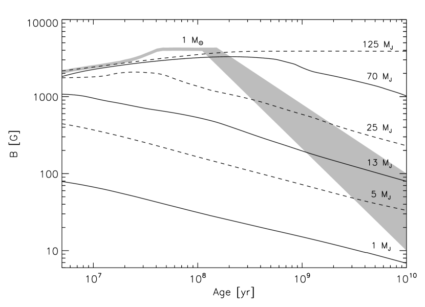
Figure 1: Average magnetic field on the surface of the object, $B_{\rm dyn}$, for $M>13$ M_J, and dipole field, $B_{\rm dip}^{\rm pol}$, for $M\leq 13$ M_J, as a function of age for giant planets, brown dwarfs, and a very-low mass star with $M=$125 M${}_{\textrm{J}}$. All low-mass objects are assumed to be rapidly rotating. An estimate of the average magnetic field of the Sun is overplotted (gray shaded area; for today’s average field see Schrijver, 1987).

We show the evolution of the magnetic fields in Fig. 1. For stars and brown dwarfs, i.e., objects with masses higher than 13 M_J, we show the average magnetic field of the dynamo, $B_{\rm dyn}$, which is probably similar to the average surface field. For giant planets, we plot the dipole field at the surface, $B_{\rm dip}$, from Eq. 2. Evolutionary tracks for a few planetary mass objects and brown dwarfs are shown, as well as one model of a very-low mass star (125 M${}_{\textrm{J}}$). In addition, we overplot an estimate of the magnetic history of the Sun. The difference between solar evolution and all other cases considered is that the Sun developes a radiative core and suffers substantial rotational braking so that it falls below the saturation threshold velocity for the dynamo. During the first $\sim 10^{8}$ yrs of its lifetime, the Sun was rotating rapidly enough so that its dynamo operated in the saturated regime captured by our scaling law. After that time, the solar rotation slowed down (e.g., Skumanich, 1972; Barnes, 2007) and magnetic field generation probably weakened in proportion to angular velocity. Evidence for such a rotation-magnetic field relation was found in M dwarfs (see Reiners et al., 2009a ). We mark this region in grey in Fig. 1 because the uncertainties in the regime of slow rotation are different from our problem and should not be discussed here. In contrast to sun-like stars, fully convective stars do not seem to suffer substantial rotational braking with the result that, even at an age of several Gyrs, they are rotating in the critical regime for magnetic field generation (Delfosse et al., 1998; Barnes, 2007; Reiners & Basri, 2008).

4.1 Evolution of magnetic fields and radio flux

The average magnetic fields of giant planets and brown dwarfs according to our scenario can vary by about an order of magnitude and more during the lifetime of the objects. The magnetic field strength is higher when the objects are young and more luminous (Eq. 1). For example, a one Jupiter-mass planet is predicted to have a polar dipole field strength on the order of $100$ G during the first few Million years; the field weakens over time and is less than 10 G after 10 Gyr. A planet with five Jupiter masses has a magnetic field at the surface that is consistently stronger by a factor of four to five over the entire evolutionary history.

Because of the higher luminosity that is essentially available for magnetic flux generation, magnetic fields in brown dwarfs are larger than fields on extrasolar giant planets, varying typically between a few kG and a hundred G depending on age and mass. Magnetic fields in brown dwarfs also weaken over time as brown dwarfs cool and loose luminosity as the power source for magnetic field generation. Low-mass stars show a generally different behaviour. A low-mass star with $M=125$ M${}_{\textrm{J}}$ can produce a magnetic field of about 2 kG during the first ten Myr, and the field grows by about a factor of two until it stays constant from an age of a few hundred Myrs on. For the solar case, the magnetic field is roughly constant between $5\,10^{7}$ and $10^{8}$ yrs, which is maintained by the constant luminosity and rapid rotation.

4.2 Comparison to other field predictions

Magnetic field estimates for extrasolar giant planets are available from a variety of different scaling laws. Christensen, (2009) summarized scaling laws for planetary magnetic fields that were proposed by different authors. Most of them assume a strong relation between field strength and rotation rate. As an example, Sánchez-Lavega, (2004) estimated the dipolar magnetic moments of exoplanets using the “Elsasser number” scaling law, which predicts the field to depend on the square root of the rotation rate but assumes no dependence on the energy flux. Sánchez-Lavega, (2004) predicts average magnetic fields of $\sim$ 30–60 G for rapidly rotating planets and $\sim 1$ G for slowly rotating ones. The range of values is comparable to our predictions. If young planets were generally fast rotators while old planets rotate slowly, which could be the case when tidal braking plays a role, the results would be similar. However, our model predicts that energy flux rules the magnetic field strength so that extrasolar giant planets have high magnetic fields during their youth and weak magnetic fields at higher ages even if their rotational evolution is entirely different (given that their are still rotating fast enough for dynamo saturation).

Stevens, (2005) used a very simplistic method to scale the magnetic fields of extrasolar giant planets assuming that the planetary magnetic moment is proportional to the planetary mass. This implies no difference between magnetic fields in young and old planets, and no difference between rapid and slow rotators (but note that slow rotators were explicitly left out of his analysis). Stevens, (2005) also provides radio flux predictions that we compare to our predictions in the next section.

4.3 Radio flux and field predictions for known planets

We have calculated the radio flux and cutoff emission frequency for the known planets of stars within 20 pc and with X-ray detections. Planet parameters are from The Extrasolar Planets Encyclopaedia. The results are given in Table 4.3 and are plotted in Fig. 2. Stevens, (2005) assumes the peak radio flux occurs at the electron cyclotron frequency of the equatorial surface field, i.e. at half the cutoff frequency. We mark the frequency range, $(0.1-1)f_{ce}$, over which significant radio emission can be expected for each planet by horizontal lines in Fig. 2. The extension of the range to lower frequencies is rather arbitrary but indicative for the emission from most of the planets of our solar system (e.g., Zarka, 1992). We include only planets that are more massive than about 0.5 M_Jup because in Saturn-sized or smaller planets helium separation may lead to stable stratification at the top of the electrical conducting region (Stevenson, 1980). The associated reduction of the surface field strength is difficult to quantify.

Table 1: Parameters of known planets around stars with X-ray detections within 20 pc

Planet Name	Planet mass	$a$	d1	$\dot{M}$	Age	$B_{\rm dip}^{\rm pol}$	radio flux1	$f_{\rm ce}$
	[${\rm M_{Jup}}\sin{i}$]	[AU]	[pc]	[$\dot{M_{\odot}}$]	[Gyr]	[G]	[mJy]	[MHz]
Jupiter	1.00	5.20		1.0	4.5	9	4.E+09	27
eps Eridani b	1.55	3.39	3.2	25.9	1.7	19	6.3	53
Gliese 876 b	1.93	0.21	4.7	0.1	2.4	23	3.1	66
Gliese 876 c	0.56	0.13	4.7	0.1	2.4	6	2.1	16
GJ 832 b	0.64	3.40	4.9	0.2	2.0	7	0.1	19
HD 62509 b	2.90	1.69	10.3	0.3	5.6	24	0.1	68
Gl 86 b	4.01	0.11	11.0	9.4	2.9	40	43.8	113
HD 147513 b	1.00	1.26	12.9	150.4	0.8	15	4.1	43
ups And b	0.69	0.06	13.5	20.2	1.4	10	41.8	27
ups And c	1.98	0.83	13.5	20.2	1.4	30	2.8	84
ups And d	3.95	2.51	13.5	20.2	1.4	58	1.0	163
gamma Cephei b	1.60	2.04	13.8	1.1	3.6	16	0.1	44
51 Peg b	0.47	0.05	14.7	0.2	6.2	3	0.8	7
tau Boo b	3.90	0.05	15.0	198.5	0.8	58	692.2	161
HR 810 b	1.94	0.91	15.5	103.9	0.8	30	5.5	83
HD 128311 b	2.18	1.10	16.6	39.9	0.9	33	2.1	92
HD 128311 c	3.21	1.76	16.6	39.9	0.9	48	1.5	134
HD 10647 b	0.91	2.10	17.3	22.9	1.4	14	0.3	38
GJ 3021 b	3.32	0.49	17.6	170.2	0.8	49	19.5	138
HD 27442 b	1.28	1.18	18.1	1.9	2.7	14	0.1	39
HD 87883 b	1.78	3.60	18.1	2.6	3.3	19	0.0	54
HD 189733 b	1.13	0.03	19.3	17.3	1.7	14	57.1	39
HD 192263 b	0.72	0.15	19.9	7.1	2.5	8	2.4	23

¹The distance to Jupiter was set to 5.2 AU for the calculation of its radio flux.

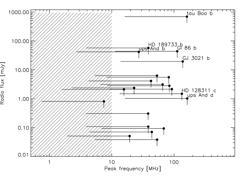
Figure 2: Radio flux for the extrasolar planets of Table 4.3. For each planet, the expected radio flux at Earth is plotted for the frequency range $(0.1-1)f_{\rm ce}$, which is the expected range of strong emission as in the case of Jupiter. The hatched area marks the frequency range below the ionospheric cutoff.

The maximum radio flux predicted for known extrasolar planets is about 700 mJy in the case of $\tau$ Boo b. Maximum emission frequencies are between 7 and 160 MHz, i.e., in most cases above the ionospheric cutoff frequency of 10 MHz. However, when the maximum frequency is less than 20 MHz the peak radio emission may fall below the ionospheric cutoff. The predicted flux for planets other than $\tau$ Boo b is at least an order of magnitude smaller. The fluxes for $\upsilon$ And b, Gl 86 b, and HD 189733 b fall into the range of 40-60 mJy, and their maximum frequencies are well above the ionospheric cutoff. For GJ 3012 b we predict 20 mJy, and all other planets fall below 10 mJy.

Our predicted radio flux values are similar to those in Stevens, (2005), which is mainly due to the fact that the distance to the object is an important factor in the observed radio emission, and that we use the same assumptions for the stellar mass loss rate. Our Fig. 2 can be compared to Figs. 1–3 in Grießmeier et al., 2007a . In general, the range of radio frequencies and radio flux are comparable but can differ substantially between individual objects. Note that we only show estimates for the planets within 20 pc. These are the most likely candidates for the detection of radio emissions.

5 Summary and Discussion

We applied the energy flux scaling relation from Christensen et al., (2009) to estimate the magnetic field evolution on giant extrasolar planets and brown dwarfs. This magnetic field scaling is independent of the rotation of the objects given that they rotate above a critical rotation limit, which probably is the case for isolated brown dwarfs, for young exoplanets, and for exoplanets in orbits not too close to their central star. Close-in planets suffer tidal braking. This applies to all candidate planets for which we predict a radio flux above 10 mJy, except GJ 3021 b. However, for planets that are very close to their host star the synchronous rotation rate may still lie above the critical limit. The critical period is on the order of four days in M-dwarfs, and if we assume the that the critical limit is somewhat higher, the top candidate for the detection of radio emissions, $\tau$ Boo b (3.3 d), as well as $\upsilon$ And b (4.6 d) and HD 189733 b (2.2 d) rotate rapidly enough. At this point, we cannot say more about the real critical limit. Gl 86 b (15.8 d) is probably rotating too slowly and our magnetic field and radio flux estimates are likely too high.

Because energy flux scales with luminosity, young exoplanets have magnetic fields about an order of magnitude higher than old exoplanets. Brown dwarfs go through a similar evolution but may go through a temporal magnetic field maximum depending on the details of the luminosity and radius evolution. Very low-mass stars build up their magnetic fields during the first few $10^{6}$ years and maintain a constant magnetic field during their entire lifetime as long as they are not efficiently braked. The latter is consistent with observations of Zeeman splitting in FeH lines, which directly yields a measurements of the average magnetic field (Reiners & Basri, 2007).

So far, no Zeeman measurements were successful in old brown dwarfs. On the other hand, Hallinan et al., (2008, and references therein) confirms the observation of electron cyclotron masers on three ultra-cool dwarfs that are probably brown dwarfs older than a few hundred Myr. This means, these ultra-cool dwarfs emit radio emission by a mechanism similar to the one discussed for planets in this paper. In particular, from radio detections at 4.88 GHz and 8.44 GHz, Hallinan et al. conclude that these brown dwarfs have regions of magnetic fields with $B>1.7$ kG and $B>3$ kG, respectively. All three objects are high-mass brown dwarfs (0.06 – 0.08 M_⊙) older than a few hundred Million years. The (average) magnetic field prediction for this class of objects is $\sim 3$ kG from our models, which is in good agreement with the observations. Another prediction from our model is that old brown dwarfs at several Gyr age have weaker fields. This needs to be tested in other (older) objects, which requires good estimates of the ages of (old) brown dwarfs. Furthermore, measurements at other radio frequencies are desirable in order to better constraint their maximum field strength.

Reiners et al., 2009b failed to detect kG-strength magnetic fields in four young ($\la 10$ Myr) accreting brown dwarfs that are rapidly rotating ($v\,\sin{i}>5$ km s^-1). According to our scenario, the objects should have average magnetic fields of 1–2 kG, but upper limits of about one kG are found in all of them. This may be a hint for a deviation from our scaling law suggesting that brown dwarfs do not follow this rule, at least not at ages below $\sim 10$ Myr. Another alternative is that (at least in brown dwarfs) the average magnetic field may be altered by the presence of an accretion disk (depending on the position of the X-point and the amount of trapped flux; see Mohanty & Shu, 2008).

Radio flux predictions for giant exoplanets based on our scaling relation are not dramatically different from earlier estimates by Farrell et al., (1999), Stevens, (2005), and Grießmeier et al., 2007a . Still, the uncertainties in the predicted radio flux are much larger than the actual values. First, our assumption of a homogenous magnetic field interacting with an isotropic wind is certainly oversimplified. Quantitative uncertainties of our flux estimates mainly come from uncertainties in the dipole moment (we estimate a factor of 3) and in the mass-loss rate (another factor of 3). Individual values of the radio flux are therefore uncertain by at least a factor of 5, but differential comparison between the radio flux predictions are likely to be more trustworthy because the objects are in general rather comparable.

We estimate that only few extrasolar planets may emit radio flux larger than 10 mJy; $\tau$ Boo b is the strongest potential emitter with $P\sim 700$ mJy. The maximum emission frequencies are well above the ionospheric cutoff frequency of 10 MHz in most cases so that detections of radio emission should not be hampered by the ionosphere.

The uncertainties of magnetic field and radio emission predictions are still very large. Nevertheless, several different scaling scenarios now exist and the one of Christensen et al., (2009) was shown to successfully reproduce magnetic fields of both planets and stars. The detection of magnetic fields in giant extrasolar planets through other techniques like the Zeeman effect will probably remain out of reach for a few decades, at least in old planets with fields that are probably well below 100 G. However, very young and massive planets may harbor magnetic fields up to one kilo-Gauss, which may become detectable in a few systems in the near future.

Radio emission from extrasolar planets has not been detected so far, but the technology for a detection may become soon available with facilities like LOFAR and others. Our scaling relation favors a different set of planets than that suggested by Grießmeier et al., 2007a although $\tau$ Boo b remains the most obvious choice. Our scaling relation can easily be applied to extrasolar planets that will be detected in the future, and target selection for radio observation campaigns can be based on these predictions.