Non existence of a phase transition for the Penetrable Square Wells in one dimension

Abstract

Penetrable Square Wells in one dimension were introduced for the first time in [A. Santos et. al., Phys. Rev. E, 77, 051206 (2008)] as a paradigm for ultra-soft colloids. Using the Kastner, Schreiber, and Schnetz theorem [M. Kastner, Rev. Mod. Phys., 80, 167 (2008)] we give strong evidence for the absence of any phase transition for this model. The argument can be generalized to a large class of model fluids and complements the van Hove’s theorem.

1 Introduction

The Penetrable Square Well (PSW) model in one dimension was first introduced in [1] as a good candidate to describe star polymers in regimes of good and moderate solvent under dilute conditions. The issue of Ruelle’ s thermodynamic stability was analyzed and the region of the phase diagram for a well defined thermodynamic limit of the model was identified. A detailed analysis of its structural and thermodynamical properties where then carried through at low temperatures [2] and high temperatures. [3]

The problem of assessing the existence of phase transitions for this one dimensional model had never been answered in a definitive way. Several attempt to find a gas-liquid phase transition were carried through using the Gibbs Ensemble Monte Carlo (GEMC) technique [4, 5, 6, 7, 8] but all gave negative results. Now it is well known that in three dimensions the Square Well (SW) model admits for a particular choice of the well parameters a gas-liquid transition. [9] As the van Hove’s theorem shows, [10, 12, 13, 11] this disappears in one dimension. Nonetheless the PSW model in one dimension, being a non nearest neighbors fluid, is not analytically solvable and since we have no hard core the van Hove’s theorem does not hold anymore. It is then interesting to answer the question whether a phase transition is possible for it. We should also mention that we also used the GEMC technique to probe for the transition in the three dimensional PSW and we generally found that for a given well width there is a penetrability threshold above which the gas-liquid transition disappears.

In the present work we use the Kastner, Schreiber, and Schnetz (KSS) theorem [14, 15] to give strong analytic evidence for the absence of any phase transition for this fluid model.

The argument hinges on a theorem of Szegö [16] on Toeplitz matrices and can be applied to a large class of one dimensional fluid models and complement the van Hove’s theorem.

The paper is organized as follows: in Section 2 we state the KSS theorem for the exclusion of phase transitions, in Section 3 we describe the PSW model, in Section 4 we show numerically that the PSW model satisfies KSS theorem, in Section 5 we show analytically that the PSW model satisfies the KSS theorem, the conclusive remarks are presented in Section 6.

2 The KSS theorem

The Kastner, Schreiber, and Schnetz (KSS) theorem [14, 15] states the following.

Theorem KSS: Let $V_{N}:\Gamma_{N}\subseteq\mathbb{R}^{N}\rightarrow\mathbb{R}$ be a smooth potential; an analytic mapping from the configuration space $\Gamma_{N}$ onto the reals. Let us indicate with ${\cal H}^{N}({\bf q})$ the Hessian of the potential. Indicating with ${\bf q}_{c}$ the critical points (or saddle points) of $V_{N}({\bf q})$ (i.e. $\nabla_{\bf q}V_{N}|_{{\bf q}={\bf q}_{c}}=0$), with $k({\bf q}_{c})$ their index (the number of negative eigenvalues of ${\cal H}^{N}({\bf q}_{c})$). Assume that the potential is a Morse function (i.e. the determinant of the Hessian calculated on all its critical points is non zero). Whenever $\Gamma_{N}$ is noncompact, assume $V_{N}$ to be “confining”, i.e. $\lim_{\lambda\to\infty}V_{N}(\lambda{\bf q})=\infty,~{}~{}~{}\forall 0\neq{\bf q}\in\Gamma_{N}$. Consider the Jacobian densities,

$$j_{l}(v)=\lim_{N\to\infty}\frac{1}{N}\ln\left[\frac{\sum_{{\bf q}_{c}\in Q_{l}([v,v+\epsilon])}J({\bf q}_{c})}{\sum_{{\bf q}_{c}\in Q_{l}([v,v+\epsilon])}1}\right]~{},$$ (1)

where

$$J({\bf q}_{c})=\left|\det\frac{{\cal H}^{N}({\bf q}_{c})}{2}\right|^{-1/2}~{},$$ (2)

and

$$Q_{l}(v)=\left\{{\bf q}_{c}|[V_{N}({\bf q}_{c})/N=v]\wedge[k({\bf q}_{c})=l(\mbox{\rm mod}4)]\right\}~{}.$$ (3)

Then a phase transition in the thermodynamic limit is excluded at any potential energy in the interval $(\bar{v}-\epsilon,\bar{v}+\epsilon)$ if: (i.) the total number of critical points is limited by $\exp(CN)$, with $C$ a positive constant, (ii.) for all sufficiently small $\epsilon$ the Jacobian densities are $j_{l}(\bar{v})<+\infty$ for $l=0,1,2,3$.

Generally the number of critical points of the potential grows exponentially with the number of degrees of freedom of the system. The fact that the total number of critical points is limited by an exponential is thought to be generically valid. [17] We then assume that for Morse potentials the first hypothesis of the theorem is satisfied. So the key hypothesis of the theorem is the second one, which can be reformulated as follows: for all sequences of critical points ${\bf q}_{c}$ such that $\lim_{N\to\infty}V_{N}({\bf q}_{c})/N=\bar{v}$, we have

$$\lim_{N\to\infty}|\det{\cal H}^{N}({\bf q}_{c})|^{\frac{1}{N}}\neq 0~{}.$$ (4)

3 The PSW model

The pair potential of the PSW model can be found as the $l\to\infty$ limit of the following continuous potential

$$\phi_{l}(r)=a[b-\tanh(l(r-1))]+c[\tanh(l(r-\lambda))+1]~{},$$ (5)

where $a=(\epsilon_{r}+\epsilon_{a})/2$, $b=(\epsilon_{r}-\epsilon_{a})/(\epsilon_{r}+\epsilon_{a})$, $c=\epsilon_{a}/2$, with $\epsilon_{r}$ a positive constant which represent the degree of penetrability of the particles, $\epsilon_{a}$ a positive constant representing the depth of the attractive well, and $\lambda=1+\Delta$, with $\Delta$ the width of the attractive square well. The Penetrable Spheres (PS) in one dimension are obtained as the $\Delta\to 0$ limit of the PSW model. In the limit of $\epsilon_{r}\to\infty$ the PSW reduces to the SW model.

The PSW model is Ruelle stable for $\epsilon_{r}/\epsilon_{a}>2(n+1)$ with $n\leq\Delta<n+1$. [1, 3]

Let us consider a pair potential of the following form

$$\Phi_{l}(r)=\phi_{l}\left(2\left(\frac{L}{2\pi}\right)^{2}\left[1-\cos\left(2\pi\frac{r}{L}\right)\right]\right)~{}.$$ (6)

Note that this pair potential is periodic of period $L$ and flat at the origin, $\Phi_{l}^{{}^{\prime}}(0)=0$. Moreover in the large $L$ limit $\Phi_{l}(r)\approx\phi_{l}(r^{2})$. In Fig. 1 we show this potential for different choices of the smoothing parameter $l$.

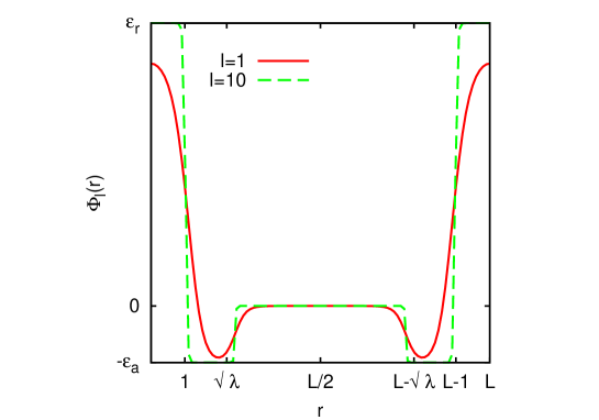
Figure 1: Shows the potential $\Phi_{l}(|x|)$ for $L\gg 1$. In the plot we used $\epsilon_{r}=5,\epsilon_{a}=1,\Delta=4,$ and $L=10$, at two values of the smoothing parameter $l$.

4 Absence of a phase transition

In this section we will apply the KSS theorem to give numerical evidence that there is no phase transition for the PSW model introduced above.

The total potential energy is

$$V_{N}({\bf q})=\frac{1}{2}\sum_{i,j=1}^{N}\Phi_{l}(|x_{i}-x_{j}|)~{},$$ (7)

where ${\bf q}=(x_{1},x_{2},\ldots,x_{N})$. If $\lim_{N\to\infty}V_{N}({\bf q})/N=v$ one finds $\epsilon_{r}/2-\epsilon_{a}\leq v<+\infty$.

The saddle points ${\bf q}_{s}=(x_{1}^{s},x_{2}^{s},\ldots,x_{N}^{s})$ for the total potential energy $(\nabla_{\bf q}V_{N}=0)$, can be various. We will only consider critical point of the following kind: equally spaced points at fixed density $\rho=N/L$,

$$x_{i}^{\rho}=i/\rho~{},~{}~{}~{}i=0,1,2,\ldots,N-1~{}.$$ (8)

Here we can reach

$$\lim_{N\to\infty}V_{N}({\bf q}_{\rho})/N=v_{\rho}~{},$$ (9)

where for large $N$ and up to an additive constant $-\phi_{l}(0)/2$ we have,

$$v_{\rho}\approx\sum_{i=0}^{N-1}\phi_{l}\left(2\left(\frac{L}{2\pi}\right)^{2}\left[1-\cos\left(\frac{2\pi i}{N}\right)\right]\right)~{}.$$ (10)

If $\rho\gg 1$, in the big $N$ limit we can approximate the sum by an integral so that

$$v_{\rho} \approx \frac{N}{2\pi}\int_{0}^{2\pi}\phi_{l}\left(2\left(\frac{L}{2\pi}\right)^{2}(1-\cos\alpha)\right)\,d\alpha$$ (11)

$$= \frac{N}{\pi}\int_{0}^{2}\frac{\phi_{l}\left(2\left(\frac{L}{2\pi}\right)^{2}x\right)}{\sqrt{1-(1-x)^{2}}}\,dx~{},$$

keeping in mind that $L=N/\rho$ and $N$ is big we find in the $l\to\infty$ limit

$$v_{\rho} \approx \frac{N}{\pi}\{\epsilon_{r}[-\arcsin(1-z)]_{0}^{1/[2(L/2\pi)^{2}]}-\epsilon_{a}[-\arcsin(1-z)]_{1/[2(L/2\pi)^{2}]}^{\lambda/[2(L/2\pi)^{2}]}\}$$ (12)

$$\approx 2\rho[\epsilon_{r}-\epsilon_{a}(\sqrt{\lambda}-1)]=v_{\rho}^{0}~{},$$

where we used for small $z$, $\arcsin(1-z)=\pi/2-\sqrt{2z}+O[z^{3/2}]$.

For small $\rho$ in the $l\to\infty$ limit you get,

$$v_{\rho} = \epsilon_{r}/2~{},~{}~{}~{}\rho<1/\sqrt{\lambda}$$ (13)

$$v_{\rho} = \epsilon_{r}/2-\epsilon_{a}~{},~{}~{}~{}1/\sqrt{\lambda}<\rho<1$$ (14)

For intermediate values of the density you will get a stepwise function of the density. A graph of $v_{\rho}$ is shown in Fig. 2.

Other stationary points would be the ones obtained by dividing the interval $L$ into $p=N/\alpha$ ($\alpha>1$) equal pieces and placing $\alpha$ particles at each of the points $x_{i}^{N,p}=iL/p$, $i=0,\ldots,p-1$. By doing so we can reach $\lim_{N\to\infty}V_{N}({\bf q}_{N,p})/N=v_{N,p}$ where up to an additive constant $-\phi_{l}(0)/2$ we have

$$v_{N,p}\approx\left(\frac{N}{p}\right)\sum_{i=0}^{p-1}\phi_{l}\left(2\left(\frac{L}{2\pi}\right)^{2}\left[1-\cos\left(\frac{2\pi i}{p}\right)\right]\right)~{}.$$ (15)

We then immediately see that for $\rho\gg\alpha$, $\lim_{N\to\infty}v_{N,p}=v_{\rho}^{0}$ but for small $\rho$, $v_{N,p}>v_{\rho}$.

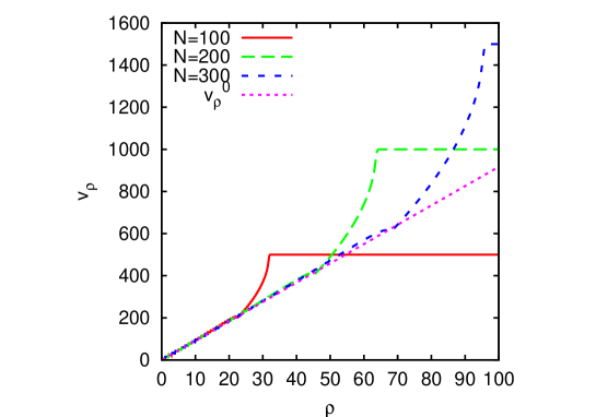
Figure 2: Shows the behavior of $v_{\rho}$ as a function of the density $\rho$ for $N=100,200,$ and $300$ when $\epsilon_{r}=5,\epsilon_{a}=1,$ and $\lambda=2$ with $l=100$. Also the theoretical prediction $v_{\rho}^{0}$ at big densities (Eq. (12)) is shown. Notice that at fixed $N$, $v_{\rho}$ will saturate to $\approx N\epsilon_{r}$ for $4(L/2\pi)^{2}<1$ or $\rho>N/\pi$.

The Hessian ${\cal H}_{i,j}^{N}({\bf q})=\partial^{2}V_{N}({\bf q})/\partial x_{i}\partial x_{j}$ calculated on the saddle points of the first kind can be written as

$${\cal H}_{i,j}^{N}({\bf q}_{\rho}) = -\Phi_{l}^{{}^{\prime\prime}}(r_{ij})~{},~{}~{}~{}i\neq j~{},$$ (16)

$${\cal H}_{i,i}^{N}({\bf q}_{\rho}) = \sum_{j\neq i}^{N}\Phi_{l}^{{}^{\prime\prime}}(r_{ij})~{},$$ (17)

where $\Phi_{l}^{{}^{\prime\prime}}(r)$ is the second derivative of $\Phi_{l}(r)$ and $r_{ij}=|i-j|/\rho$.

So the Hessian calculated on the saddle point is a circulant symmetric matrix with one zero eigenvalue due to the fact that we have translational symmetry $x_{i}^{\rho}=x_{i}^{\rho}\pm n/\rho$ for any $i$ and any integer $n$. In order to break the symmetry we need to fix one point for example the one at $x_{N}^{\rho}$. So the Hessian becomes a $(N-1)\times(N-1)$ symmetric Toeplitz matrix (non circulant anymore) which we call $\bar{{\cal H}}^{(N-1)}({\bf q}_{\rho})$.

In Fig. 3 we have calculated the $|\det\bar{{\cal H}}^{N}({\bf q}_{\rho})|^{1/N}$ as a function of $N$ at $\rho=N/L$ fixed for $\epsilon_{a}=1,\epsilon_{r}=5,\Delta=1$, and $l=10$. One can see that the normalized determinant of the Hessian does not go to zero in the large $N$ limit. So the Kastner, Schreiber, and Schnetz (KSS) criteria [14, 15] is not satisfied and a phase transition is excluded. The same holds for the PS model.

In Fig. 4 we show the dependence of $|\det\bar{{\cal H}}^{N}({\bf q}_{\rho})|^{1/N}$ on density for different choices of $N$.

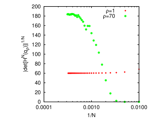
Figure 3: Shows the behavior of $|\det\bar{{\cal H}}^{N}({\bf q}_{\rho})|^{1/N}$ as a function of $N$ at two different densities. Here we chose $\epsilon_{a}=1,\epsilon_{r}=5,\Delta=1$, and $l=10$.

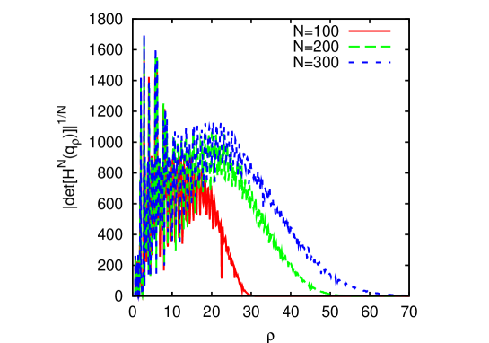
Figure 4: Shows the behavior of $|\det\bar{{\cal H}}^{N}({\bf q}_{\rho})|^{1/N}$ as a function of $\rho$ for various $N$. Here we chose $\epsilon_{a}=1,\epsilon_{r}=5,\Delta=1$, and $l=10$. Notice that for $\rho\lesssim 1/\sqrt{\lambda}$ then ${\cal H}^{N}({\bf q}_{\rho})\approx 0$ and also the normalized determinant is very small. While the approach to zero at large densities is an artifact of the finite sizes of the systems considered.

A system where there is a phase transition has been proved to be the self-gravitating ring (SGR) [18] where $\phi_{SGR}(r)=-1/\sqrt{r+2(L/2\pi)^{2}\epsilon}$. In this case one finds $v_{\rho}^{0}=-\rho 2\sqrt{2/\epsilon}{\cal A}(2/\epsilon)$, with ${\cal A}(x)=\int_{0}^{\pi/2}d\theta\,(1+x\sin^{2}\theta)^{-1/2}$. They use Hadamard upper bound to the absolute value of a determinant to prove that indeed $\lim_{N\to\infty}|\det\bar{{\cal H}}^{N}({\bf q}_{\rho})|^{1/N}=0$. In Fig. 5 we show this numerically for a particular choice of the parameters. Actually this result could be expected from what will be proven in the next section, as in the large $N$ limit for any finite $\epsilon$, $\phi_{SGR}=o(1/N)$ and $|\det\bar{{\cal H}}^{N}({\bf q}_{\rho})|^{1/N}=o(1/N)$. This is a confirmation that theorem KSS is not violated.

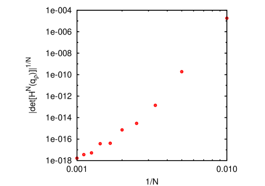
Figure 5: Shows the behavior of $|\det\bar{{\cal H}}^{N}({\bf q}_{\rho})|^{1/N}$ as a function of $N$ for fixed $\rho=1$ in a bilogarithmic plot. Here we chose $\epsilon=0.1$.

5 Limit of the normalized determinant

In this section we will give analytical evidence that there cannot be a phase transition for the PSW model.

We need to apply to our case, Szegö’s theorem [16] for sequences of Toeplitz matrices which deals with the behavior of the eigenvalues as the order of the matrix goes to infinity. In particular we will be using the following Proposition.

Proposition: Let $T_{n}=\{t^{n}_{kj}|k,j=0,1,2,\ldots,n-1\}$ be a sequence of Toeplitz matrices with $t^{n}_{kj}=t^{n}_{k-j}$ such that $T=\lim_{n\to\infty}T_{n}$ and $t_{k}=\lim_{n\to\infty}t^{n}_{k}$ for $k=0,1,2\ldots$. Let us introduce

$$f(x)=\sum_{k=-\infty}^{\infty}t_{k}\,e^{ikx}~{},~{}~{}~{}x\in[0,2\pi]~{}.$$ (18)

Then there exists a sequence of Toeplitz matrices $\tilde{T}_{n}=\{\tilde{t}_{kj}|k,j=0,1,2,\ldots,n-1\}$ with $\tilde{t}_{kj}=\tilde{t}_{k-j}$ and

$$\tilde{t}_{k}=\frac{1}{2\pi}\int_{0}^{2\pi}f(x)e^{-ikx}\,dx~{},$$ (19)

such that

$$\lim_{n\to\infty}|\det T_{n}|^{1/n}=\lim_{n\to\infty}|\det\tilde{T}_{n}|^{1/n}=\exp\left(\frac{1}{2\pi}\int_{0}^{2\pi}\ln|f(x)|\,dx\right)~{},$$ (20)

as long as the integral of $\ln|f(x)|$ exists finite.

If the Toeplitz matrix is Hermitian then $t_{-k}=t_{k}^{*}$ and $f$ is real valued. If moreover The Toeplitz matrix is symmetric then $t_{-k}=t_{k}$ and additionally $f(x)=f(2\pi-x)$.

By choosing $T_{N}=\bar{{\cal H}}^{N}({\bf q}_{\rho})$ and calling $t^{N}_{i-j}={\cal H}_{i,j}^{N}({\bf q}_{\rho})$ we have in the $N\to\infty$ limit, with $L=N/\rho$ ($\rho$ constant), $t_{k}=\lim_{N\to\infty}t^{N}_{k}$ and

$$f(x) = \lim_{\stackrel{{\scriptstyle N\to\infty}}{{N\,{\rm odd}}}}\left(2\sum_{k=1}^{(N-1)/2}t^{N}_{k}\cos(kx)+t^{N}_{0}\right)$$ (21)

$$= 2\sum_{k=1}^{\infty}t_{k}\cos(kx)+t_{0}~{},$$

$$t^{N}_{k} = -\Phi_{l}^{{}^{\prime\prime}}(k/\rho)~{},~{}~{}~{}k=1,2,\ldots,(N-1)/2~{},$$ (22)

$$t^{N}_{0} = -2\sum_{k=1}^{(N-1)/2}t^{N}_{k}~{},$$ (23)

So that $f(0)=0$. Notice that in this case the sequence of matrices $\bar{{\cal H}}^{N}({\bf q}_{\rho})$ does not coincide with the sequence used in the Proposition, only the limiting matrix for large $N$ coincides. But since Szegö’s theorem states the limit of the normalized determinant exists it should be independent from the sequence chosen. An additional support to the Proposition is presented in A.

Now in order to prove the absence of a phase transition we need to prove that $\int_{0}^{2\pi}\ln|f(x)|\,dx$ does not diverge to minus infinity. That is we must control the way $f$ passes through zero. In particular we do not want to have that if $x_{0}$ is a zero of $f$ then

$$|f(x)|\sim e^{-1/|x-x_{0}|^{\alpha}}~{},~{}~{}~{}x\sim x_{0}~{},$$ (24)

with $\alpha\geq 1$, which is faster than any finite power of $(x-x_{0})$.

Now for PSW we can write $\Phi_{l}(r)=\Phi_{l}^{core}(r)+\Phi_{l}^{tail}(r)$. Choose $\Phi_{l}^{tail}(r)=\alpha\exp(-2lr^{2})$ with $\alpha=(\epsilon_{a}+\epsilon_{r})e^{2l}-\epsilon_{a}e^{2\lambda l}$. It is then always possible to redefine the starting potential $\Phi_{l}(r)$ in such a way that $\Phi_{l}^{core}(r)$ exactly vanishes for $r\geq r_{cut}>\sqrt{\lambda}$ keeping all the derivatives at $r=r_{cut}$ continuous. Now in Eq. (21) for $f^{core}$ only a finite number of $k$ contributes to the series, namely the ones for $1\leq k<\rho r_{cut}$. So $f^{core}$ will be well behaved on its zeroes. For the tail we get $f^{tail}(x)=-\alpha\sqrt{\pi/2l}x^{2}\exp(-x^{2}/8l)$. So that we will never have $|f(x)|$ going through a zero (note that the zeroes of $f$ increase in number as $\rho$ increases) with the asymptotically fast behavior of Eq. (24). This proves the absence of any phase transition for the PSW (or PS) models.

Note that the argument continues to hold for example for the Gaussian Core Model (GCM) [19] defined by $\phi_{GCM}(r)=\epsilon\exp[-(r/\sigma)^{2}]$. In this case by choosing $\phi(r)=\exp(-r)$ we get in the large $L$ limit $\Phi(r)=\exp(-r^{2})$ and the Fourier transform of $\Phi^{{}^{\prime\prime}}(r)$ is $-\sqrt{\pi}x^{2}\exp(-x^{2}/4)$ which poses no problems for the zero of $f(x)$ at $x=0$ (note that in this case $f(x)$ is always positive for $x>0$).

The argument breaks down for example if $f(x)=-\exp(-1/|x|)$. In this case the pair potential will be given by $\Phi(r)\sim-\int_{-\infty}^{\infty}\exp(ixr)f(x)/x^{2}\,dx$, and one finds $\Phi(r)\sim 2[\sqrt{-ir}K_{1}(2\sqrt{-ir})+\sqrt{ir}K_{1}(2\sqrt{ir})]$, where $K_{n}$ is the modified Bessel function of the second kind. See Fig. 6 for a plot. Also the relevant feature, in the pair potential, which gives the break down of the argument for the absence of a phase transition, is the large $r$ behavior. Notice that in this case we numerically found out that the normalized determinant tend to a finite value for large $N$. In accord with the fact that when the hypotheses of the proposition are not satisfied Eq. (20) looses its meaning. Considering the normalized determinant for the rescaled potential $\Phi(r)/h(N)$, with $h(N)\to+\infty$ as $N\to\infty$, we saw that it indeed tends to zero, indicating the presence of a phase transition.

We simulated this model fluid and indeed we found that it undergoes a gas-liquid phase transition. The coexisting binodal curve is shown in Fig. 7 and in Table 1 we collect various properties of the two phases. We used GEMC in which two systems can exchange both volume and particles (the total volume $V$ and the total number of particles $N$ are fixed) in such a way to have the same pressures and chemical potentials. We constructed the binodal for $N=50$ particles. In the simulation we had $2N$ particle random displacements (with a magnitude of $0.5\sigma_{i}$, where $\sigma_{i}$ is the dimension of the simulation box of system $i$), $N/10$ volume changes (with a random change of magnitude $0.1$ in $\ln[V_{1}/(V-V_{1})]$, where $V_{1}$ is the volume of one of the two systems), and $N$ particle swap moves. We observed that in order to obtain the binodals at different system sizes we had to assume a scaling of the following kind: $\beta N^{\alpha}=\beta_{50}50^{\alpha}=$constant, indicating that the model is not Ruelle stable (as it may be expected since it has a bounded core and a large attractive region), and $\rho N=\rho_{50}50=$constant, where $\beta_{50}$ and $\rho_{50}$ are the coexistence data shown in Fig. 7 and Table 1. For $50\lesssim N\lesssim 100$ we found $\alpha\approx 1/2$, for $N\approx 200$ then $\alpha\approx 2/3$, and for $N\approx 300$ then $\alpha\approx 3/4$.

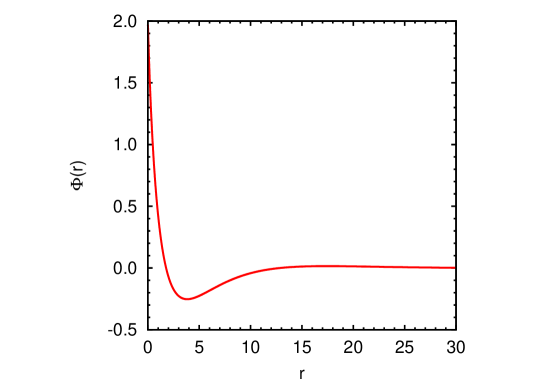
Figure 6: Shows the pair potential $\Phi(r)=2[\sqrt{-ir}K_{1}(2\sqrt{-ir})+\sqrt{ir}K_{1}(2\sqrt{ir})]$ of the counterexample given in the text. We have $\Phi(0)=2$ and $\Phi(r)\propto\sin\sqrt{2r}\exp(-\sqrt{2r})$ at large $r$.

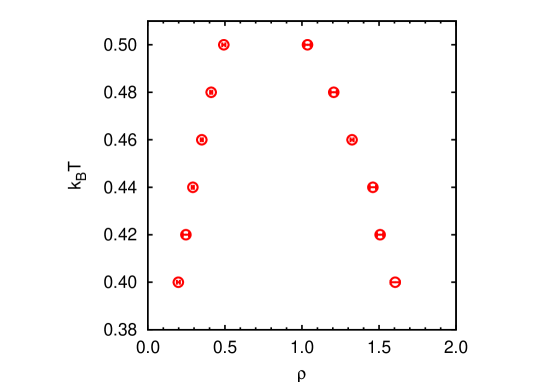
Figure 7: Shows the gas-liquid coexistence line in the temperature density plane, obtained with the GEMC for $N=50$ particles [20] interacting with the pair potential of Fig. 6.

$k_{B}T$	$\rho_{v}$	$\rho_{l}$	$u_{v}$	$u_{l}$	$-(3\ln\Lambda)/\beta+\mu_{v}$	$-(3\ln\Lambda)/\beta+\mu_{l}$
0.40	0.20 $\pm$0.01	1.61 $\pm$0.03	-0.224 $\pm$0.009	-0.907 $\pm$0.007	-0.97 $\pm$0.01	-0.97 $\pm$0.01
0.42	0.25 $\pm$0.02	1.51 $\pm$0.02	-0.26 $\pm$0.01	-0.873 $\pm$0.008	-0.95 $\pm$0.01	-0.943 $\pm$0.008
0.44	0.292 $\pm$0.007	1.46 $\pm$0.02	-0.290 $\pm$0.007	-0.854 $\pm$0.004	-0.938 $\pm$0.004	-0.921 $\pm$0.006
0.46	0.350 $\pm$0.007	1.32 $\pm$0.01	-0.340 $\pm$0.004	-0.815 $\pm$0.006	-0.90 $\pm$0.01	-0.89 $\pm$0.02
0.48	0.411 $\pm$0.007	1.21 $\pm$0.02	-0.370 $\pm$0.003	-0.77 $\pm$0.01	-0.886 $\pm$0.003	-0.86 $\pm$0.01
0.50	0.49 $\pm$0.01	1.04 $\pm$0.02	-0.420 $\pm$0.006	-0.71 $\pm$0.01	-0.87 $\pm$0.01	-0.862 $\pm$0.006

Table 1: Gas-liquid coexistence data ($T,\rho_{i},u_{i},\mu_{i}$ are respectively the temperature the density, the internal energy per particle, and the chemical potential of the vapor $i=v$ or liquid $i=l$ phase. $\beta=1/k_{B}T$ and $\Lambda$ is the de Broglie thermal wavelength.) from GEMC of $N=50$ particles [20].

We then added an hard core to the potential

$$\Phi(r)=\left\{\begin{array}[]{ll}\epsilon&r<1\\ 2[\sqrt{-ir}K_{1}(2\sqrt{-ir})+\sqrt{ir}K_{1}(2\sqrt{ir})]&r\geq 1\end{array}\right.~{},$$ (27)

with $\epsilon$ a positive large number, and we saw, through GEMC, that the corresponding fluid still admitted a gas-liquid phase transition (without $N$ scaling of the densities $\rho<1$) in accord with the expectation that are the large $r$ tails of the potential that make this model singular from the point of view of our argument.

For fluids with a pair potential $\Phi$ given by a hard core and a $-1/r^{\alpha}$ tail we can take the $\Phi^{{}^{\prime\prime}}(r)=0$ for $r<1$ and $\Phi^{{}^{\prime\prime}}(r)=-\alpha(\alpha-1)/r^{\alpha-2}$ for $r>1$, and the resulting $f$ function (the Fourier transform of $-\Phi^{{}^{\prime\prime}}$) is such that $\ln|f(x)|$ has non-integrable zeros. So this class of models does not fall under the hypotheses pf the proposition. And it is well known that when $1<\alpha<2$ the corresponding fluid admits a phase transition [12].

6 Conclusions

Using KSS theorem and a limit theorem of Szegö on Toeplitz matrices we were able to give strong evidence for the exclusion of phase transitions in the phase diagram of the PSW (or PS) fluid. The argument makes use of the fact that the smoothed pair potential amongst the particles has an $r$ cutoff. Even if we just considered two classes of stationary points, i.e. the equally spaced points and equally spaced clusters, we believe that our argument give strong indications of the absence of a phase transition.

Our argument applies equally well to model fluids with large $r$ tails in the pair potential decaying in such a way that the condition of Eq. (24) does not hold. For example it applies to the Gaussian Core Model. We believe this to be a rather large class of fluid models.

We give an example of a model fluid which violates the condition of Eq. (24) and find through GEMC simulations that it indeed has a gas-liquid phase transition.

Our argument does not require the fluid to be a nearest neighbor one, for which it is well known that the equation of state can be calculated analytically [21, 22, 23]. We think that our argument can be a good candidate to complement the well known van Hove theorem for such systems that violates the hypotheses of the hard core impenetrability of the particles and of the compactness of the support of the tails.

Appendix A Alternative support to the Szegö result

Our original matrix ${\cal H}^{N}({\bf q}_{\rho})$ is a circulant matrix

$${\cal H}^{N}({\bf q}_{\rho})=\left(\begin{array}[]{cccccc}h^{N}_{0}&h^{N}_{1}&h^{N}_{2}&h^{N}_{3}&\cdots&h^{N}_{N-1}\\ h^{N}_{N-1}&h^{N}_{0}&h^{N}_{1}&h^{N}_{2}&\cdots&h^{N}_{N-2}\\ h^{N}_{N-2}&h^{N}_{N-1}&h^{N}_{0}&h_{1}&\cdots&h^{N}_{N-3}\\ \vdots&&&\ddots&&\vdots\\ h^{N}_{1}&h^{N}_{2}&h^{N}_{3}&h^{N}_{4}&\cdots&h^{N}_{0}\end{array}\right)~{},$$ (33)

We have numerically checked that the determinant of ${\cal H}^{N}({\bf q}_{\rho})$ with one row and one column removed converges in the large $N$ limit to the product of the non-zero eigenvalues of the matrix ${\cal H}^{N}({\bf q}_{\rho})$.

Let us assume that $N=2n+1$ is odd. Then our matrix has the following additional structure

$$h^{N}_{i} = \tilde{h}^{N}_{i}~{},~{}~{}~{}i=1,\ldots,n$$

$$h^{N}_{n+i} = \tilde{h}^{N}_{n-(i-1)}~{},~{}~{}~{}i=1,\ldots,n$$ (34)

The eigenvalues of $H^{N}$ will be given by [24]

$$\psi_{m}=\sum_{k=0}^{N-1}h^{N}_{k}e^{-\frac{2\pi}{N}imk}~{},~{}~{}~{}m=0,1,\ldots,N-1$$ (35)

with the additional constraint (see Eqs. (16)-(17)) that

$$\psi_{0}=\sum_{k=0}^{N-1}h^{N}_{k}=0~{}.$$ (36)

The eigenvalues can be rewritten as follows

$$\psi_{m}=\tilde{h}^{N}_{0}+\sum_{k=1}^{n}\tilde{h}^{N}_{k}e^{-\frac{2\pi}{N}imk}+\sum_{k=1}^{n}\tilde{h}^{N}_{n-(k-1)}e^{-\frac{2\pi}{N}im(n+k)}~{}.$$ (37)

Introducing the summation index $j=n-k+1$ in the last sum we then obtain

$$\psi_{m} = \tilde{h}^{N}_{0}+\sum_{k=1}^{n}\tilde{h}^{N}_{k}e^{-\frac{2\pi}{N}imk}+\sum_{j=n}^{1}\tilde{h}^{N}_{j}e^{+\frac{2\pi}{N}imj}$$ (38)

$$= \sum_{k=-n}^{n}t^{N}_{k}e^{-\frac{2\pi}{N}imk}~{},$$

with $n=(N-1)/2$ and $t^{N}_{k}=t^{N}_{-k}=\tilde{h}^{N}_{k}$ for $k=1,2,\ldots,n$.

We take the logarithm of the absolute value of the product of the non-zero eigenvalues to find

$${\cal P}=\frac{1}{N}\ln\left|\prod_{m=1}^{N}\psi_{m}\right|=\frac{1}{N}\sum_{m=1}^{N}\ln|\psi_{m}|~{}.$$ (39)

Now in the large $N$ limit we have $t_{k}=\lim_{N\to\infty}t^{N}_{k}$ for $k=0,1,2,\ldots$ and

$$\psi_{m} \sim \sum_{k=-\infty}^{\infty}t_{k}e^{-\frac{2\pi}{N}imk}\sim f\left(\frac{2\pi}{N}m\right)~{},$$ (40)

$${\cal P} \sim \frac{1}{N}\sum_{m=1}^{N}\ln\left|f\left(\frac{2\pi}{N}m\right)\right|\sim\frac{1}{2\pi}\int_{0}^{2\pi}\ln|f(x)|\,dx~{},$$ (41)

where in the last passage we have transformed the sum into an integral.

References

References

[1]
A. Santos, R. Fantoni, and A. Giacometti.
Phys. Rev. E, 77:051206, 2008.
[2]
R. Fantoni, A. Giacometti, A. Malijevský, and A. Santos.
J. Chem. Phys., 131:124106, 2009.
[3]
R. Fantoni, A. Giacometti, A. Malijevský, and A. Santos.
J. Chem. Phys., 2010.
to appear.
[4]
D. Frenkel and B. Smit.
Understanding Molecular Simulation.
Academic Press, San Diego, 1996.
[5]
A. Z. Panagiotopoulos.
Mol. Phys., 61:813, 1987.
[6]
A. Z. Panagiotopoulos, N. Quirke, M. Stapleton, and D. J. Tildesley.
Mol. Phys., 63:527, 1988.
[7]
B. Smit, Ph. De Smedt, and D. Frenkel.
Mol. Phys., 68:931, 1989.
[8]
B. Smit and D. Frenkel.
Mol. Phys., 68:951, 1989.
[9]
Hongjun Liu, Shekhar Garde, and Sanat Kumar.
J.Chem. Phys., 123:174505, 2005.
[10]
L. van Hove.
Physica (Amsterdam), 16:137, 1950.
[11]
J. A. Cuesta and A. Sánchez.
J. Stat. Phys., 115:869, 2004.
[12]
P. C. Hemmer and G. Stell.
Phys. Rev. Lett., 24:1284, 1970.
[13]
J. M. Kincaid, G. Stell, and C. K. Hall.
J. Chem. Phys., 65:2161, 1976.
[14]
Michael Kastner and Oliver Schnetz.
Phys. Rev. Lett., 100:160601, 2008.
[15]
Michael Kastner.
Rev. Mod. Phys., 80:167, 2008.
[16]
U. Grenander and G. Szegö.
Toeplitz forms and their applications.
University of California Press, Berkeley and Los Angeles, 1958.
page 65.
[17]
D. J. Wales.
Energy landscapes.
Cambridge University Press, Cambridge, England, 2004.
[18]
Cesare Nardini and Lapo Casetti.
Phys. Rev. E, 80:060103, 2009.
[19]
P. J. Flory and W. R. Krigbaum.
J. Chem. Phys., 18:1086, 1950.
[20]
The Monte Carlo simulations where carried on at the Center for High Performance
Computing (CHPC), CSIR Campus, 15 Lower Hope St., Rosebank, Cape Town, South
Africa. Manufacturer: IBM e1350 Cluster, CPU: AMD Opteron, CPU Clock: 2.6
GHz, CPU Cores: 2048, Memory: 16GB, Peak Performance: 3.3 TFlops, Storage: 94
TB (Multicluster), Launch date: 2007.
[21]
Z. W. Salsburg, R. W. Zwanzig, and J. G. Kirkwood.
J. Chem. Phys., 21:1098, 1953.
[22]
D. S. Corti and P. G. Debenedetti.
Phys. Rev. E, 57:4211, 1998.
[23]
M. Heying and D. S. Corti.
Fluid Phase Equilibria, 220:85, 2004.