A strongly degenerate parabolic
aggregation equation

Abstract.

This paper is concerned with a strongly degenerate convection-diffusion equation in one space dimension whose convective flux involves a non-linear function of the total mass to one side of the given position. This equation can be understood as a model of aggregation of the individuals of a population with the solution representing their local density. The aggregation mechanism is balanced by a degenerate diffusion term accounting for dispersal. In the strongly degenerate case, solutions of the non-local problem are usually discontinuous and need to be defined as weak solutions satisfying an entropy condition. A finite difference scheme for the non-local problem is formulated and its convergence to the unique entropy solution is proved. The scheme emerges from taking divided differences of a monotone scheme for the local PDE for the primitive. Numerical examples illustrate the behaviour of entropy solutions of the non-local problem, in particular the aggregation phenomenon.

1. Introduction

1.1. Scope

This paper is related to the initial value problem for a strongly degenerate convection-diffusion equation of the form

$$u_{t}+\left(\Phi^{\prime}\biggl{(}\int_{-\infty}^{x}u(y,t)\,\mathrm{d}y\biggr{)}u(x,t)\right)_{x}=A(u)_{xx},\quad x\in\mathbb{R},\quad 0<t\leq T,$$ (1.1)

$$u(x,0)=u_{0}(x)\geq 0,\quad x\in\mathbb{R},\quad u_{0}\in(L^{1}\cap L^{\infty})(\mathbb{R})$$ (1.2)

for the density $u=u(x,t)\geq 0$, where $A(u)$ is a diffusion function given by

$$A(u):=\int_{0}^{u}a(s)\,\mathrm{d}s,\quad\text{where $a(u)\geq 0$ for $u\in\mathbb{R}$}.$$ (1.3)

The model (1.1), (1.2) was studied as a model of aggregation by a series of authors including Alt [1], Diaz, Nagai, and Shmarev [8], Nagai [21] and Nagai and Mimura [22, 23, 24], all of which assumed that $a(u)=0$ at most at isolated values of $u$. It is the purpose of this paper to study (1.1), (1.2) under the more general assumption that $a(u)=0$ on bounded $u$-intervals on which (1.1) reduces to a first-order conservation law with non-local flux. We assume that

$$A(u)\to\infty\quad\text{as $u\to\infty$.}$$ (1.4)

This implies that $a(\cdot)$ may vanish only on bounded subintervals of $\mathbb{R}$.

The key observation made in previous work [1, 21, 22, 23, 24] is that if all coefficient functions are sufficiently smooth, and $u(x,t)$ is an $L^{1}$ solution of the problem (1.1), (1.2), then the primitive (precisely, of $u(\cdot,t)$) defined by

$$v(x,t):=\int_{-\infty}^{x}u(\xi,t)\,\mathrm{d}\xi,\quad t\in(0,T],$$ (1.5)

is a solution of the local initial value problem

$$v_{t}+\Phi(v)_{x}=A(v_{x})_{x},\quad x\in\mathbb{R},\quad t\in(0,T],$$ (1.6)

$$v(x,0)=v_{0}(x),\quad x\in\mathbb{R},\quad v_{0}(x):=\int_{-\infty}^{x}u_{0}(\xi)\,\mathrm{d}\xi.$$ (1.7)

As a non-linear but local PDE, (1.6) is more amenable to well-posedness and numerical analysis. In this work we use that the transformation to the local equation (1.6) is also possible in the strongly degenerate case, in which solutions of (1.1) are usually discontinuous and need to be defined as weak solutions. To achieve uniqueness, an additional selection criterion is imposed, and the type of solutions sought are (Kružkov-type) entropy solutions. The core, and essential novelty, of the paper is the formulation and convergence proof of a finite difference scheme for (1.1), (1.2) (in short, “$u$-scheme”). The scheme is based on a monotone difference scheme for the initial value problem (1.6), (1.7) (in short, “$v$-scheme”) in the strongly degenerate case, which in turn is a special case of the schemes formulated and analyzed by Evje and Karlsen [11] for the more general doubly degenerate equation $v_{t}+\Phi(v)_{x}=B(A(v_{x}))_{x}$. The $u$-scheme is obtained by taking finite differences of the numerical solution values generated by the $v$-scheme.

The $v$-scheme is, in particular, monotonicity preserving, so the discrete approximations for $v$ are always monotonically increasing when the initial datum $v_{0}$ is, and therefore the $u$-scheme produces non-negative solutions. Moreover, by modifications of standard compactness and Lax-Wendroff-type arguments it is proved that the numerical approximations generated by the $u$-scheme converge to the unique entropy solution of (1.1), (1.2). An appealing feature is that the primitive (1.5) never needs to be calculated explicitly (except for the computation of $v_{0}$). Numerical examples illustrate the behaviour of entropy solutions of (1.1), (1.2), and recorded error histories demonstrate the convergence of the $v$- and $u$-schemes.

1.2. Assumptions

We assume that $u_{0}$ has compact support, and that there exists a constant $\mathcal{M}$ such that

$$\operatorname*{TV}(u_{0})<\mathcal{M}.$$ (1.8)

We also need that $\Phi\in C^{2}(\mathbb{R})$, and that $\Phi$ has exactly one maximum:

$$\exists v^{*}\in\mathbb{R}:\quad\Phi^{\prime}(v^{*})=0,\quad\Phi^{\prime}(v)>0\;\text{for $v<v^{*}$},\quad\Phi^{\prime}(v)<0\;\text{for $v>v^{*}$}.$$ (1.9)

This assumption is introduced to facilitate some of the steps of our analysis; it is, however, not essential. In fact, in our convergence analysis of Section 4 we need to discuss the local behaviour of the numerical solution for $v$ close to where it includes the value $v^{*}$ since that value is critical in the definition of the numerical flux. If we employ a function $\Phi$ that has several separate extrema, then the locations of solution values including extrema are spatially well separated since the discrete analogue of $v_{x}$ is bounded, and the techniques of Section 4 can be extended to that case in a straightforward manner.

1.3. Motivation and related work

Equation (1.1), or some specific cases of it, were studied in a series of papers [1, 8, 21, 22, 23, 24], in all of which it is assumed that $a(\cdot)$ vanishes at most at isolated values of its argument, so that it is always ensured that $A^{\prime}(u)>0$ for $u\geq 0$. The interpretation of (1.1) as a model of the aggregation of populations (e.g., of animals) advanced in those papers is also valid here and can be illustrated as follows. Assume that $u(x,t)$ is the density of the population under study, and consider the equation

$$u_{t}+\left(-k\left[\int_{-\infty}^{x}u(y,t)\,\mathrm{d}y-\int_{x}^{\infty}u(y,t)\,\mathrm{d}y\right]u\right)_{x}=A(u)_{xx},\quad k>0.$$ (1.10)

Here, the convective term provides a mechanism that moves $u(x,t)$ to the right (respectively, to the left) if

$$\int_{-\infty}^{x}u(y,t)\,\mathrm{d}y<\int_{x}^{\infty}u(y,t)\,\mathrm{d}y\quad\text{(respectively, $\ldots>\ldots$)}.$$

In other words, an animal will move to the right (respectively, left) if the total population to its right is larger (respectively, smaller) than to its left. Now assume that the initial population is finite and define

$$C_{0}:=\int_{\mathbb{R}}u_{0}(x)\,\mathrm{d}x.$$ (1.11)

It is then clear that (1.10) is an example of (1.1) if $\Phi^{\prime}(v)=-k(2v-C_{0})$, i.e.,

$$\Phi(v)=-kv(v-C_{0})+\mathrm{const.}$$ (1.12)

The aggregation mechanism is balanced by nonlinear diffusion described by the term $A(u)_{xx}$, termed density-dependent dispersal in mathematical ecology. A typical novel feature addressed by the present analysis is a “threshold effect”, i.e. dispersal only sets on when the density $u$ exceeds a critical value $u_{\mathrm{c}}>0$, i.e.

$$a(u)\begin{cases}=0&\text{if $u\leq u_{\mathrm{c}}$, $u_{\mathrm{c}}>0$,}\\ >0&\text{if $u>u_{\mathrm{c}}$}.\end{cases}$$

More recently, spatially multi-dimensional aggregation equations of the form

$$u_{t}+\nabla\cdot(u\nabla K\ast u)=\Delta A(u)$$ (1.13)

have seen an enormous amount of interest, where the typical case treated in literature is $A\equiv 0$. Here, $K$ denotes an interaction potential, and $K\ast u$ denotes spatial convolution. For overviews we refer to [3, 18, 25]. The non-local and diffusive term account for long-range and short-range interactions, respectively, as is emphasized in [5]. The derivation of (1.13) from microscopic interacting particle systems and related models, and for particular choices of $K$ and $A$, is presented in [2, 4, 5, 19, 20]. Related models also include equations with fractional dissipation that cannot be cast in the form (1.13), see e.g. [16, 17].

The essential research problem associated with (1.13) (or variants of this equation) is the well-posedness of this equation together with bounded initial data $u(x,0)=u_{0}(x)$ for $x\in\mathbb{R}^{d}$, where $d$ denotes the number of space dimensions. While the short-time existence of a unique smooth solution for smooth intial data is known in most situations, one wishes to determine criteria in terms of the functions $K$ and $A$ (or related diffusion terms), and possibly of $u_{0}$, that either ensure that smooth solutions exist globally in time, or that compel that solutions of (1.13) will blow up in finite time. This problem is analyzed in [2, 3, 4, 5, 6, 16, 17, 18] (this list is far from being complete).

The occurrence of blow-up was analyzed in terms of the properties of $K$ for $A\equiv 0$ in [2, 3]; if $K$ is a radial function, i.e., $K=K(|x|)$, then blow-up occurs if the Osgood condition for the characteristic ODEs is violated, as occurs e.g. for $K(x)=\exp(-|x|)$, while for a $C^{2}$ kernel this does not occur [2]. Li and Rodrigo [16, 17] consider this particular kernel and describe the circumstances under which blow-up occurs if the aggregation equation is equipped with fractional diffusion.

The present equation (1.1) can be written as a one-dimensional version of (1.13) only in special cases. However, and as was already pointed out in [22], (1.10) can be written as

$$u_{t}+(u\tilde{K}\ast u)_{x}=A(u)_{xx}$$ (1.14)

with the odd kernel $\smash{\tilde{K}(x)=-k\operatorname*{sgn}(x)}$. Equation (1.14) becomes a one-dimensional example of (1.13) if we observe that $\smash{\tilde{K}\ast u=K^{\prime}\ast u}$, where $K^{\prime}$ denotes the derivative of $K$, if we choose the even kernel

$$K(x)=-k|x|+C,$$ (1.15)

where $C$ is a constant. We can write this as $K(x)=-\kappa(|x|)$ for $\kappa(r)=r-C$. Suppose that one uses this kernel in the multi-dimensional equation (1.13). It is then straightforward to verify that in absence of dispersal ($A\equiv 0$), the kernel (1.15) satisfies the integral condition for blow-up in finite time, see [2]. One result of our analysis is then that a strongly degenerate diffusion term $A(u)_{xx}$, accounting for dispersal, is sufficient to prevent blow-up of solutions of (1.13) provided that the condition (1.4) is satisfied. In fact, in the context of aggregation models that are based either on (1.1) or on the more recently studied equation (1.13), the present work is the first that incorporates a strongly degenerate diffusion term, i.e. involves a function $A(u)$ that is flat on a $u$-interval of positive length. So far, diffusion terms that have been considered in (1.1) degenerate at most at isolated $u$-values. Nagai and Mimura [22] studied the Cauchy problem for equation (1.1) under the assumptions $A(0)=0$, $A^{\prime}(u)>0$ being an odd function. The initial function for the Cauchy problem in [22] is assumed to be bounded, non-negative and integrable. They prove existence and uniqueness of a bounded and continuous solution to the initial-value problem. In [23] the asymptotic behaviour of solutions to the same problem was studied for the specific choice

$$A(u)=u^{m},\quad m>1.$$ (1.16)

It seems that the analysis of (1.13) with degenerate diffusion has just started. Li and Zhang [18] study this equation in one space dimension for the diffusion function $A(u)=u^{3}/3$, which degenerates at $u=0$ only. On the other hand, the numerical simulations presented herein show that under strongly degenerate diffusion, typical features of the aggregation phenomenon such as “clumped” solutions with very sharp edges [25] appear.

Finally, we comment that there is also considerable interest in the well-posedness and other properties of the local PDE (1.6) (or variants of this equation) under the assumption that $A(\cdot)$ is an increasing but bounded function, an effect usually denoted by saturating diffusion, cf. [7] and references cited in that paper. In this case, which is explicitly excluded by our assumption (1.4), $v_{x}$ (though not necessarily $v$ itself) becomes in general unbounded. It is at present unclear whether well-posedness of our nonlocal problem (1.1), (1.2) can also be achieved under saturating diffusion.

1.4. Outline of the paper

The remainder of this paper is organized as follows. In Section 2 we state the definition of an entropy solution of (1.1), (1.2), and point out that an entropy solution is also a weak solution. In Section 3.1 we state jump conditions that can be derived from the definition of an entropy solution, and in Section 3.2 we prove the uniqueness of an entropy solution.

Section 4 presents a convergence analysis for the $u$-scheme, which in part relies on standard compactness properties for the $v$-scheme. In Section 4.1, the schemes are described. Section 4.2 contains a series of lemmas stating uniform estimates on the numerical approximations generated by the $v$- and the $u$-schemes, which allow to employ standard compactness arguments to deduce that both schemes converge.

The final convergence result (Theorem 4.1) and its proof are presented in Section 4.3. This proof involves a discrete cell entropy satisfied by the $u$-scheme, which eventually permits to conclude that $\smash{\{u_{j-1/2}^{n}\}}$ converges to an entropy solution as the discretization parameters tend to zero. This means, in particular, that an entropy solution exists. The mathematical model and the $v$- and $u$-scheme are illustrated by numerical examples presented in Section 5.

2. Definition of an entropy solution

Definition 2.1.

A measurable, non-negative function $u$ is an entropy solution of the initial value problem (1.1), (1.2) if it satisfies the following conditions:

1. We have $u\in L^{\infty}(\Pi_{T})\cap L^{1}(\Pi_{T})\cap L^{\infty}(0,T;BV(\mathbb{R}))\cap C(0,T;L^{1}(\mathbb{R}))$, and $A(u)\in L^{2}(0,T;H^{1}(\mathbb{R}))$.

2. The initial condition (1.2) is satisfied in the following sense:

   $$\lim_{t\downarrow 0}\int_{\mathbb{R}}\bigl{|}u(x,t)-u_{0}(x)\bigr{|}\,\mathrm{d}x=0.$$ (2.1)

3. For all non-negative test functions $\varphi\in C_{0}^{\infty}(\Pi_{T})$, the entropy inequality

   $$\begin{split}\forall k\in\mathbb{R}:\iint_{\Pi_{T}}&\Bigl{\{}|u-k|\bigl{(}\varphi_{t}+\Phi^{\prime}(v)\varphi_{x}\bigr{)}-\operatorname*{sgn}(u-k)uk\Phi^{\prime\prime}(v)\varphi\\ &+\bigl{|}A(u)-A(k)\bigr{|}\varphi_{xx}\Bigr{\}}\,\mathrm{d}x\,\mathrm{d}t\geq 0\end{split}$$ (2.2)

   is satisfied, where $v(x,t)$ is defined by (1.5) and $\Pi_{T}:=\mathbb{R}\times(0,T)$.

Definition 2.2.

A measurable function $u$ is said to be a weak solution of the initial value problem (1.1), (1.2) if it satisfies items (1) and (2) of Definition 2.1 and if the following equality is satisfied for all test functions $\phi\in C_{0}^{\infty}(\Pi_{T})$:

$$\begin{split}\iint_{\Pi_{T}}&\Bigl{\{}u\bigl{(}\phi_{t}+\Phi^{\prime}(v)\phi_{x}\bigr{)}+A(u)\phi_{xx}\Bigr{\}}\,\mathrm{d}x\,\mathrm{d}t=0.\end{split}$$ (2.3)

It is straightforward to check that an entropy solution of the initial value problem (1.1), (1.2) is, in particular, a weak solution.

Lemma 2.1.

Assume that $u$ is an entropy solution of the initial value problem (1.1)–(1.2) (cf. Definition 2.1). Then $u$ is a weak solution (cf. Definition 2.2).

Proof.

Choosing $\smash{k\geq\|u\|_{L^{\infty}(\Pi_{T})}}$ in (2.2) we obtain

$$\iint_{\Pi_{T}}\Bigl{\{}-(u-k)\bigl{(}\phi_{t}+\Phi^{\prime}(v)\phi_{x}\bigr{)}-A(u)\phi_{xx}\Bigr{\}}\,\mathrm{d}x\,\mathrm{d}t\geq-k\iint_{\Pi_{T}}u\Phi^{\prime\prime}(v)\phi\,\mathrm{d}x\,\mathrm{d}t$$

or equivalently,

$$\begin{split}&\iint_{\Pi_{T}}\Bigl{\{}u\bigl{(}\phi_{t}+\Phi^{\prime}(v)\phi_{x}\bigr{)}+A(u)\phi_{xx}\Bigr{\}}\,\mathrm{d}x\,\mathrm{d}t\\ &\leq k\iint_{\Pi_{T}}\Bigl{\{}\phi_{t}+\bigl{(}\Phi^{\prime}(v)\phi\bigr{)}_{x}\Bigr{\}}\,\mathrm{d}x\,\mathrm{d}t=0.\end{split}$$ (2.4)

On the other hand, since we look for non-negative solutions, it suffices to set $k=0$ in (2.2) to deduce that we always have

$$\iint_{\Pi_{T}}\Bigl{\{}u\bigl{(}\phi_{t}+\Phi^{\prime}(v)\phi_{x}\bigr{)}+A(u)\phi_{xx}\Bigr{\}}\,\mathrm{d}x\,\mathrm{d}t\geq 0.$$ (2.5)

Combining (2.4) and (2.5) we see that $u$ satisfies (2.3). ∎

3. Jump conditions and uniqueness

3.1. Rankine-Hugoniot condition and entropy jump condition

Assume that $u$ is an entropy solution having a discontinuity at a point $(x_{0},t_{0})\in\Pi_{T}$ between the approximate limits $u^{+}$ and $u^{-}$ of $u$ taken with respect to $x>x_{0}$ and $x<x_{0}$, respectively. Standard results from the theory of entropy solutions of strongly degenerate parabolic equations imply that such a discontinuity is possible only if $A(u)$ is flat for $u\in\mathcal{I}(u^{-},u^{+}):=[\min\{u^{-},u^{+}\},\max\{u^{-},u^{+}\}]$. In that case, the propagation velocity of the jump is given by the Rankine-Hugoniot condition, which is derived by standard arguments from the weak formulation (2.3):

$$s=\frac{1}{u^{+}-u^{-}}\Bigl{(}\Phi^{\prime}(v^{+})u^{+}-\Phi^{\prime}(v^{-})u^{-}-\bigl{(}A(u)_{x}\bigr{)}^{+}+\bigl{(}A(u)_{x}\bigr{)}^{-}\Bigr{)}.$$ (3.1)

Here, $\smash{(A(u)_{x})^{+}}$ and $\smash{(A(u)_{x})^{-}}$ denote the approximate limits of $A(u)_{x}$ taken with respect to $x>x_{0}$ and $x<x_{0}$, respectively, and $v^{+}$ and $v^{-}$ denote the corresponding limits of $v(x,t)$. However, since $v(x,t)$ is continuous, we actually have $v^{+}=v^{-}$, and the Rankine-Hugoniot condition (3.1) reduces to

$$s=\Phi^{\prime}\bigl{(}v(x_{0},t_{0})\bigr{)}-\frac{(A(u)_{x})^{+}-(A(u)_{x})^{-}}{u^{+}-u_{-}}.$$ (3.2)

In addition, a discontinuity between two solution values needs to satisfy the jump entropy condition

$$\begin{split}&\forall k\in\bigl{(}\min\{u^{-},u^{+}\},\max\{u^{-},u^{+}\}\bigr{)}:\\ &\displaystyle{\frac{{\displaystyle{\Phi^{\prime}(v^{+})(u^{+}-k)-(A(u)_{x})^{+}}}}{{\displaystyle{u^{+}-k}}}}\leq s\leq\displaystyle{\frac{{\displaystyle{\Phi^{\prime}(v^{-})(u^{-}-k)-(A(u)_{x})^{-}}}}{{\displaystyle{u^{-}-k}}}}.\end{split}$$ (3.3)

Taking into account $v^{+}=v^{-}$ and (3.2), this reduces to

$$\begin{split}&\forall k\in\bigl{(}\min\{u^{-},u^{+}\},\max\{u^{-},u^{+}\}\bigr{)}:\\ &\displaystyle{\frac{{\displaystyle{(A(u)_{x})^{+}}}}{{\displaystyle{u^{+}-k}}}}\geq\frac{(A(u)_{x})^{+}-(A(u)_{x})^{-}}{u^{+}-u_{-}}\geq\displaystyle{\frac{{\displaystyle{(A(u)_{x})^{-}}}}{{\displaystyle{u^{-}-k}}}}.\end{split}$$ (3.4)

In particular, if $A(\cdot)$ is flat on an open interval containing $\mathcal{I}(u^{-},u^{+})$, then the double inequality (3.4) is trivially satisfied. That $\Phi(v)$ is smooth, greatly simplifies the jump and entropy jump conditions.

3.2. Uniqueness of entropy solutions

The uniqueness of entropy solutions is an immediate consequence of a result proved in [14] (cf. also [12]) regarding continuous dependence of entropy solutions with respect to the flux function. More precisely, we have

Theorem 3.1.

There exists at most one entropy solution (according to Definition2.1) of the initial value problem (1.1), (1.2). Moreover, there exists a constant $C=C\left(\max|\Phi^{\prime}|\right)$ such that

$$\bigl{\|}u(\cdot,t)-\bar{u}(\cdot,t)\bigr{\|}_{L^{1}(\mathbb{R})}\leq C\|u_{0}-\bar{u}_{0}\|_{L^{1}(\mathbb{R})},\qquad\forall t\in(0,T],$$

where $u$ and $\bar{u}$ are entropy solutions with initial data $u_{0}$ and $\bar{u}_{0}$, respectively.

Proof.

Let $u$ be an entropy solution of the problem

$$u_{t}+\bigl{(}V(x,t)u\bigr{)}_{x}=A(u)_{xx},\qquad V(x,t):=\Phi^{\prime}\left(\int_{-\infty}^{x}u(y,t)\,\mathrm{d}y\right),$$

with initial data $u(0,x)=u_{0}(x)$, and let $\bar{u}$ be an entropy solution of the problem

$$\bar{u}_{t}+\left(\bar{V}(x,t)\bar{u}\right)_{x}=A(\bar{u})_{xx},\qquad\bar{V}(x,t):=\Phi^{\prime}\left(\int_{-\infty}^{x}\bar{u}(y,t)\,\mathrm{d}y\right).$$

with initial data $\bar{u}(0,x)=\bar{u}_{0}(x)$. According to [12, 13], keeping in mind that $u$ and $\bar{u}$ are of bounded variation, i.e., $u,\bar{u}\in L^{\infty}(0,T;BV(\mathbb{R}))$, there exists a constant $C$ such that

$$\bigl{\|}u(\cdot,t)-\bar{u}(\cdot,t)\bigr{\|}_{L^{1}(\mathbb{R})} \leq\|u_{0}-\bar{u}_{0}\|_{L^{1}(\mathbb{R})}+\int_{0}^{t}\bigl{|}V_{x}(x,s)-\bar{V}_{x}(x,s)\bigr{|}\,\mathrm{d}s$$

$$\qquad\qquad\qquad+\int_{0}^{t}\bigl{|}V(x,s)-\bar{V}(x,s)\bigr{|}\operatorname*{TV}(u(\cdot,s))\,\mathrm{d}s$$

$$\leq\|u_{0}-\bar{u}_{0}\|_{L^{1}(\mathbb{R})}+C\int_{0}^{t}\bigl{|}V_{x}(x,s)-\bar{V}_{x}(x,s)\bigr{|}\,\mathrm{d}s.$$

Observe that

$$\int_{0}^{t}\bigl{|}V_{x}(x,s)-\bar{V}_{x}(x,s)\bigr{|}\,\mathrm{d}s\leq\max|\Phi^{\prime}|\int_{0}^{t}\bigl{|}u(x,s)-\bar{u}(x,s)\bigr{|}\,\mathrm{d}s,$$

so that by the Gronwall inequality we arrive at

$$\bigl{\|}u(\cdot,t)-\bar{u}(\cdot,t)\bigr{\|}_{L^{1}(\mathbb{R})}\leq\exp{\left(\max|\Phi^{\prime}|\,t\right)}\|u_{0}-\bar{u}_{0}\|_{L^{1}(\mathbb{R})}.$$

∎

4. Convergence analysis of numerical schemes

4.1. Preliminaries

We define the vectors $\smash{U^{n}:=\{u_{j+1/2}^{n}\}_{j\in\mathbb{Z}}}$ and $\smash{V^{n}:=\{v_{j}^{n}\}_{j\in\mathbb{Z}}}$, and discretize $\mathbb{R}$ by $x_{j}:=j\Delta x$, $j\in\mathbb{Z}$, and the time interval $[0,T]$ by $t_{n}=n\Delta t$, $n=0,\dots,N$, $\Delta t:=T/N$, $N\in\mathbb{N}$. We denote by $\smash{u_{j+1/2}^{n}}$ the cell average over $\smash{I_{j}:=[x_{j},x_{j+1}]}$ at time $t_{n}$ and $j\in\mathbb{Z}$. We also define $\lambda:=\Delta t/\Delta x$ and $\smash{\mu:=\Delta t/\Delta x^{2}=\lambda/\Delta x}$ and wherever convenient use the spatial difference operators $\smash{\Delta_{+}\phi_{j}:=\phi_{j+1}-\phi_{j}}$, $\smash{\Delta_{-}\phi_{j}:=\phi_{j}-\phi_{j-1}}$, and

$$\Delta^{\!2}\phi_{j}:=\Delta_{+}\Delta_{-}\phi_{j}=\phi_{j+1}-2\phi_{j}+\phi_{j-1}.$$

We assume that the initial datum $u_{0}$ is discretized via

$$u_{j+1/2}^{0}:=\frac{1}{\Delta x}\int_{I_{j}}u_{0}(\xi)\,d\xi,\quad j\in\mathbb{Z}.$$ (4.1)

Moreover, we define the operator $\mathcal{S}_{\Delta x}$ and its inverse $\smash{\mathcal{S}_{\Delta x}^{-1}}$ via

$$\mathcal{S}_{\Delta x}(U^{n};j):=\Delta x\sum_{l=-\infty}^{j-1}u_{l+1/2}^{n},\quad\mathcal{S}^{-1}_{\Delta x}(V^{n};j):=\frac{v_{j+1}^{n}-v_{j}^{n}}{\Delta x}.$$ (4.2)

Clearly, $\smash{\mathcal{S}_{\Delta x}}$ and $\smash{\mathcal{S}_{\Delta x}^{-1}}$ are the discrete analogues of the integral and differential operators that convert $u(\cdot,t_{n})$ into $v(\cdot,t_{n})$ and vice versa, respectively. Since we assume that $u_{0}$ is compactly supported, the sum in (4.2) is actually finite.

The numerical scheme for the initial value problem (1.1), (1.2) can be compactly written as follows:

$$U^{n+1}=\bigl{[}\mathcal{S}_{\Delta x}^{-1}\circ\mathcal{H}\circ\mathcal{S}_{\Delta x}\bigr{]}U^{n},\quad n=0,\dots,N-1,$$ (4.3)

where the basic idea is to utilize a standard scheme of the form

$$V^{n+1}=\mathcal{H}(V^{n}),\quad n=0,\dots,N-1$$ (4.4)

for approximate solutions of the local PDE (1.6), starting from the initial data

$$v_{j}^{0}:=\Delta x\sum_{l=-\infty}^{j-1}u_{l+1/2}^{0}=\int_{-\infty}^{x_{j}}u_{0}(\xi)\,\mathrm{d}\xi,\quad j\in\mathbb{Z}.$$

Clearly, if $C_{0}$ is the total mass defined in (1.11), then we have that

$$0\leq v_{j}^{0}\leq C_{0},\quad v_{j}^{0}\leq v_{j+1}^{0}\quad\text{for all $j\in\mathbb{Z}$.}$$ (4.5)

Let us emphasize here that (4.3) implies that

$$U^{n}=\bigl{[}\mathcal{S}_{\Delta x}^{-1}\circ\mathcal{H}\circ\mathcal{S}_{\Delta x}\bigr{]}^{n}U^{0}=\bigl{[}\mathcal{S}_{\Delta x}^{-1}\circ\mathcal{H}^{n}\circ\mathcal{S}_{\Delta x}\bigr{]}U^{0}.$$

This means that for the actual computation of $U^{n}$ from $U^{0}$, the operators $\mathcal{S}_{\Delta x}$ and $\smash{\mathcal{S}_{\Delta x}^{-1}}$ need to be applied only once, and not for every time step.

To derive properties of the scheme (4.3), we first analyze the scheme (4.4), which is here given by the marching formula

$$v_{j}^{n+1}=v_{j}^{n}-\lambda\Delta_{+}\bigl{[}h\bigl{(}v_{j-1}^{n},v_{j}^{n}\bigr{)}-A\bigl{(}\Delta_{-}v_{j}^{n}/\Delta x\bigr{)}\bigr{]},\quad j\in\mathbb{Z},\quad n=0,1,2,\dots,$$ (4.6)

where $\lambda$ is subject to the CFL condition stated below, and

$$h(w,z):=\Phi(0)+\Phi_{+}(w)+\Phi_{-}(z)$$ (4.7)

is the Engquist-Osher flux [9], where we define the functions

$$\Phi_{+}(v):=\int_{0}^{v}\max\bigl{\{}0,\Phi^{\prime}(s)\bigr{\}}\,\mathrm{d}s,\quad\Phi_{-}(v):=\int_{0}^{v}\min\bigl{\{}0,\Phi^{\prime}(s)\bigr{\}}\,\mathrm{d}s.$$ (4.8)

We assume that $\Delta t$ and $\Delta x$ satisfy the CFL stability condition

$$2\lambda\max_{u\in\mathbb{R}}\bigl{|}\Phi^{\prime}(u)\bigr{|}+2\mu\max_{u\in\mathbb{R}}\bigl{|}a(u)\bigr{|}\leq 1.$$ (4.9)

Note that the scheme for $u$ can be written as

$$u_{j+1/2}^{n+1}=u_{j+1/2}^{n}-\lambda\Delta_{+}G_{j}^{n}+\mu\Delta^{2}A\bigl{(}u_{j+1/2}^{n}\bigr{)},\quad j\in\mathbb{Z},\quad n=0,1,2,\dots,$$ (4.10)

where we define

$$G_{j}^{n}:=\displaystyle{\frac{{\displaystyle{1}}}{{\displaystyle{\Delta x}}}}\Delta_{+}h\bigl{(}v_{j-1}^{n},v_{j}^{n}\bigr{)}=\displaystyle{\frac{{\displaystyle{1}}}{{\displaystyle{\Delta x}}}}\left(\int_{v_{j-1}^{n}}^{v_{j}^{n}}\Phi_{+}^{\prime}(s)\,\mathrm{d}s+\int_{v_{j}^{n}}^{v_{j+1}^{n}}\Phi_{-}^{\prime}(s)\,\mathrm{d}s\right).$$ (4.11)

For the ease of reference, we will refer to (4.6)–(4.8) and (4.10), (4.11) as “$v$-scheme” and “$u$-scheme”, respectively.

4.2. Uniform estimates on $\{v_{j}^{n}\}$ and $\{u_{j}^{n}\}$

Lemma 4.1.

Under the CFL condition (4.9), the $v$-scheme defined by (4.6)–(4.8) is monotone.

Proof.

We rewrite the scheme (4.6) as

$$v_{j}^{n+1}=\mathcal{H}\bigl{(}v_{j-1}^{n},v_{j}^{n},v_{j+1}^{n}\bigr{)}=:\mathcal{H}_{j}^{n},\quad j\in\mathbb{Z},\quad n=0,1,\dots,N-1.$$

Since $a\geq 0$, we then have

$$\frac{\partial\mathcal{H}_{j}^{n}}{\partial v_{j\pm 1}^{n}} =\mp\lambda\min\bigl{\{}0,\Phi^{\prime}\bigl{(}v_{j\pm 1}^{n}\bigr{)}\bigr{\}}+\mu a\bigl{(}\Delta_{\pm}v_{j}^{n}/\Delta x\bigr{)}\geq 0,$$

while the CFL condition (4.9) implies that

$$\frac{\partial\mathcal{H}_{j}^{n}}{\partial v_{j}^{n}} =1-\lambda\bigl{(}\max\bigl{\{}0,\Phi^{\prime}\bigl{(}v_{j}^{n}\bigr{)}\}-\min\bigl{\{}0,\Phi^{\prime}\bigl{(}v_{j}^{n}\bigr{)}\}\bigr{)}-\mu\Delta_{+}a\bigl{(}\Delta_{-}v_{j}^{n}/\Delta x\bigr{)}$$

$$=1-\lambda\bigl{|}\Phi^{\prime}\bigl{(}v_{j}^{n}\bigr{)}\bigr{|}-\mu\Delta_{+}a\bigl{(}\Delta_{-}v_{j}^{n}/\Delta x\bigr{)}\geq 0.$$

∎

As a monotone scheme, the scheme (4.6) is total variation diminishing (TVD) and monotonicity preserving. Since (4.6) represents an explicit three-point scheme, for a fixed discretization $(\Delta x,\Delta t)$ we will always have

$$v_{j}^{n}=0\quad\text{for $j<-\mathcal{K}$},\quad v_{j}^{n}=C_{0}\quad\text{for $j>\mathcal{K}$}$$ (4.12)

for a sufficiently large constant $\mathcal{K}>0$. Thus, we can state the following corollary.

Corollary 4.1.

If (4.5) and the CFL condition (4.9) hold, then the numerical solution $\{v_{j}^{n}\}$ produced by the $v$-scheme (4.6)–(4.8) satisfies

$$0\leq v_{j}^{n}\leq C_{0},\quad v_{j}^{n}\leq v_{j+1}^{n}\quad\text{\em for all $j\in\mathbb{Z}$, $n=1,\dots,N$.}$$ (4.13)

As a direct consequence, the numerical solution values $V^{n}=\smash{\{v_{j}^{n}\}_{j\in\mathbb{Z}}}$ satisfy the (trivial) uniform total variation bound

$$\operatorname*{TV}(V^{n})=\sum_{j\in\mathbb{Z}}\left|v^{n}_{j+1}-v^{n}_{j}\right|=C_{0}.$$

Lemma 4.2.

The numerical solution $\smash{\{v_{j}^{n}\}}$ produced by the $v$-scheme (4.6)–(4.8) satisfies the $L^{1}$ Lipschitz continuity in time property, i.e., there exists a constant $C_{1}$, which is independent of $\Delta:=(\Delta x,\Delta t)$, such that

$$\sum_{j\in\mathbb{Z}}\left|v^{n+1}_{j}-v^{n}_{j}\right|\leq C_{1}\lambda.$$ (4.14)

Proof.

For $j\in\mathbb{Z}$, the quantity $\smash{w^{n+1/2}_{j}:=v^{n+1}_{j}-v^{n}_{j}}$ satisfies

$$\begin{split}w^{n+3/2}_{j}-w^{n+1/2}_{j}&=-\lambda\Delta_{+}\bigl{[}h\bigl{(}v^{n+1}_{j-1},v^{n+1}_{j}\bigr{)}-h\bigl{(}v^{n}_{j-1},v^{n}_{j}\bigr{)}\bigr{]}\\ &\quad+\lambda\Delta_{+}\bigl{[}A\bigl{(}\Delta_{-}v^{n+1}_{j}/\Delta x\bigr{)}-A\bigl{(}\Delta_{-}v^{n}_{j}/\Delta x\bigr{)}\bigr{]}.\end{split}$$ (4.15)

We define

$$\theta(s):=\begin{cases}1/s&\text{if $s\neq 0$,}\\ 0&\text{otherwise,}\end{cases}$$

and the quantities

$$\begin{split}B^{n+1/2}_{j}&:=\bigl{[}h\bigl{(}v^{n}_{j-1},v^{n+1}_{j}\bigr{)}-h\bigl{(}v^{n}_{j-1},v^{n}_{j}\bigr{)}\bigr{]}\theta\bigl{(}v^{n+1}_{j}-v^{n}_{j}\bigr{)},\\ C^{n+1/2}_{j}&:=\bigl{[}h\bigl{(}v^{n+1}_{j},v^{n+1}_{j+1}\bigr{)}-h\bigl{(}v^{n}_{j},v^{n+1}_{j+1}\bigr{)}\bigr{]}\theta\bigl{(}v^{n+1}_{j}-v^{n}_{j}\bigr{)},\\ D^{n+1/2}_{j}&:=\bigl{[}A\bigl{(}\Delta_{+}v^{n+1}_{j}/\Delta x\bigr{)}-A\bigl{(}\Delta_{+}v^{n}_{j}/\Delta x\bigr{)}\bigr{]}\theta\bigl{(}\Delta_{+}v^{n+1}_{j}-\Delta_{+}v^{n}_{j}\bigr{)}.\end{split}$$ (4.16)

Due to the monotonicity of $\smash{\{v_{j}^{n}\}}$ (see (4.13)) we have

$$C^{n+1/2}_{j}\geq 0,\quad D^{n+1/2}_{j}\geq 0,\quad B^{n+1/2}_{j}\leq 0.$$ (4.17)

After some manipulations and using (4.13) we obtain from (4.15)

$$w^{n+3/2}_{j} =w^{n+1/2}_{j}\bigl{[}1-\lambda C^{n+1/2}_{j}+\lambda B^{n+1/2}_{j}-\lambda\bigl{(}D^{n+1/2}_{j-1}+D^{n+1/2}_{j}\bigr{)}\bigr{]}$$

$$\quad+w^{n+1/2}_{j-1}\lambda\bigl{(}C^{n+1/2}_{j-1}+D^{n+1/2}_{j-1}\bigr{)}+w^{n+1/2}_{j+1}\lambda\bigl{(}-B^{n+1/2}_{j+1}+D^{n+1/2}_{j}\bigr{)}.$$

Using the CFL condition we find

$$\bigl{|}w^{n+3/2}_{j}\bigr{|} \leq\bigl{|}w^{n+1/2}_{j}\bigr{|}\bigl{[}1-\lambda\bigl{(}C^{n+1/2}_{j}-B^{n+1/2}_{j}+D^{n+1/2}_{j-1}+D^{n+1/2}_{j}\bigr{)}\bigr{]}$$

$$\quad+\bigl{|}w^{n+1/2}_{j-1}\bigr{|}\lambda\bigl{(}C^{n+1/2}_{j-1}+D^{n+1/2}_{j-1}\bigr{)}+\bigl{|}w^{n+1/2}_{j+1}\bigr{|}\lambda\bigl{(}-B^{n+1/2}_{j+1}+D^{n+1/2}_{j}\bigr{)}.$$

Summing this over $j\in\mathbb{Z}$, using (4.17) and (4.13) we obtain

$$\sum_{j\in\mathbb{Z}}\bigl{|}w^{n+3/2}_{j}\bigr{|}\leq\sum_{j\in\mathbb{Z}}\bigl{|}w^{n+1/2}_{j}\bigr{|},$$

which implies that

$$\sum_{j\in\mathbb{Z}}\bigl{|}w^{n+3/2}_{j}\bigr{|}\leq\sum_{j\in\mathbb{Z}}\bigl{|}w^{1/2}_{j}\bigr{|}.$$

From (4.6) with $n=0$ we get

$$\sum_{j\in\mathbb{Z}}\bigl{|}w^{1/2}_{j}\bigr{|} =\sum_{j\in\mathbb{Z}}\bigl{|}v^{1}_{j}-v^{0}_{j}\bigr{|}=\sum_{j\in\mathbb{Z}}\lambda\bigl{|}\Delta_{+}\bigl{(}h\bigl{(}v_{j-1}^{0},v_{j}^{0}\bigr{)}-A\bigl{(}\Delta_{-}v_{j}^{0}/\Delta x\bigr{)}\bigr{)}\bigr{|}.$$

Using (1.8) we arrive at (4.14). ∎

Lemma 4.3.

The numerical solution $\smash{\{v_{j}^{n}\}}$ produced by the $v$-scheme (4.6)–(4.8) satisfies the inequality $\smash{|\Delta_{+}v^{n}_{j}/\Delta x|\leq C_{3}}$ with a constant $C_{3}$, which is independent of $\Delta$. Equivalently, the solution $\smash{\{u_{j+1/2}^{n}\}}$ generated by the $u$-scheme (4.10), (4.11) satisfies the uniform $L^{\infty}$ bound

$$\bigl{|}u_{j+1/2}^{n}\bigr{|}\leq C_{3}\quad\text{\em for all $j\in\mathbb{Z}$, $n=0,\dots,N$.}$$ (4.18)

Proof.

It is sufficient to show that $\smash{A(\Delta_{+}v^{n}_{j}/\Delta x)\leq C_{2}}$ for a constant $C_{2}$ that is independent of $\Delta$. Taking into account (4.12) we get

$$\bigl{|}A\bigl{(}\Delta_{+}v^{n}_{j}/\Delta x\bigr{)}\bigr{|}-\bigl{|}h\bigl{(}v^{n}_{j},v^{n}_{j+1}\bigr{)}\bigr{|}$$

$$\leq\bigl{|}A\bigl{(}\Delta_{+}v^{n}_{j}/\Delta x\bigr{)}-h\bigl{(}v^{n}_{j},v^{n}_{j+1}\bigr{)}\bigr{|}$$

$$=\left|\Phi(0)+\sum^{j}_{k=-\infty}\Delta_{-}\bigl{(}A\bigl{(}\Delta_{+}v^{n}_{k}/\Delta x\bigr{)}-h\bigl{(}v^{n}_{k},v^{n}_{k+1}\bigr{)}\bigr{)}\right|$$

$$=\left|\sum^{j}_{k=-\infty}\frac{v^{n+1}_{k}-v^{n}_{k}}{\lambda}+\Phi(0)\right|\leq\displaystyle{\frac{{\displaystyle{1}}}{{\displaystyle{\lambda}}}}\sum_{k\in\mathbb{Z}}\bigl{|}v^{n+1}_{k}-v^{n}_{k}\bigr{|}+\bigl{|}\Phi(0)\bigr{|}.$$

Due to Lemma 4.2, we see that $\smash{|A(\Delta_{+}v^{n}_{j}/\Delta x)|\leq C_{2}}$ if we choose $C_{2}=C_{1}+|\Phi(0)|$. Taking into account (1.4) concludes the proof. ∎

Remark 4.1.

Under all the previous assumptions we see that the $v$-scheme (4.6)–(4.8) satisfies the following discrete cell entropy inequality

$$\left|v^{n+1}_{j}-k\right|-\left|v^{n}_{j}-k\right|+\lambda\Delta_{+}H^{n}_{j-1/2}-\lambda\operatorname*{sgn}\bigl{(}v^{n+1}_{j}-k\bigr{)}\Delta_{+}A\bigl{(}\Delta_{-}v^{n}_{j}/\Delta x\bigr{)}\leq 0,$$

where $k\in\mathbb{R}$ and a numerical entropy flux is defined by

$$H^{n}_{j+1/2}=H^{n}_{j+1/2}\bigl{(}v^{n}_{j},v^{n}_{j+1},k\bigr{)}:=h\bigl{(}v^{n}_{j}\vee k,v^{n}_{j+1}\vee k\bigr{)}-h\bigl{(}v^{n}_{j}\wedge k,v^{n}_{j+1}\wedge k\bigr{)}.$$

By a standard Lax-Wendroff-type argument we conclude that as $\Delta\to 0$, the piecewise constant functions assuming the value $\smash{v_{j}^{n}}$ on $\smash{I_{j+1/2}\times[t_{n},t_{n+1})}$ converge to a limit function $v$ that for all non-negative test functions $\varphi\in C_{0}^{\infty}(\Pi_{T})$ satisfies the entropy inequality

$$\forall k\in\mathbb{R}:\quad\iint_{\Pi_{T}}\Bigl{\{}|v-k|\varphi_{t}+\operatorname*{sgn}(v-k)\bigl{[}\Phi(v)-\Phi(k)-A(v_{x})\bigr{]}\varphi_{x}\Bigr{\}}\,\mathrm{d}x\,\mathrm{d}t\geq 0.$$

However, since under the present assumptions $v(\cdot,t)$ is a monotone smooth function, the entropy satisfaction property is not needed here.

Lemma 4.4.

The solution $\smash{\{u_{j+1/2}^{n}\}}$ generated by the $u$-scheme (4.10), (4.11) satisfies the following inequality, where the constant $C_{4}$ is independent of $\Delta$:

$$\operatorname*{TV}\bigl{(}A(U^{n})\bigr{)}=\sum_{j\in\mathbb{Z}}\bigl{|}\Delta_{+}A\bigl{(}u^{n}_{j-1/2}\bigr{)}\bigr{|}\leq C_{4}.$$

Proof.

Using the marching formula (4.6) we can write

$$\bigl{|}\Delta_{+}A\bigl{(}u^{n}_{j-1/2}\bigr{)}\bigr{|} \leq\displaystyle{\frac{{\displaystyle{1}}}{{\displaystyle{\lambda}}}}\bigl{|}v^{n+1}_{j}-v^{n}_{j}\bigr{|}+\bigl{|}\Delta_{+}h\bigl{(}v^{n}_{j-1},v^{n}_{j}\bigr{)}\bigr{|}$$

$$\leq\displaystyle{\frac{{\displaystyle{1}}}{{\displaystyle{\lambda}}}}\bigl{|}v^{n+1}_{j}-v^{n}_{j}\bigr{|}+\bigl{|}\bigl{[}h\bigl{(}v^{n}_{j},v^{n}_{j+1}\bigr{)}-h\bigl{(}v^{n}_{j},v^{n}_{j}\bigr{)}\bigr{]}\theta\bigl{(}v^{n}_{j+1}-v^{n}_{j}\bigr{)}\bigr{|}\bigl{|}\Delta_{+}v^{n}_{j}\bigr{|}$$

$$\quad+\bigl{|}\bigl{[}h\bigl{(}v^{n}_{j},v^{n}_{j}\bigr{)}-h\bigl{(}v^{n}_{j-1},v^{n}_{j}\bigr{)}\bigr{]}\theta\bigl{(}v^{n}_{j}-v^{n}_{j-1}\bigr{)}\bigr{|}\bigl{|}\Delta_{-}v^{n}_{j}\bigr{|}.$$

Summing over $j\in\mathbb{Z}$ yields

$$\sum_{j\in\mathbb{Z}}\bigl{|}\Delta_{+}A\bigl{(}u^{n}_{j-1/2}\bigr{)}\bigr{|}\leq\frac{1}{\lambda}\sum_{j\in\mathbb{Z}}\bigl{|}v^{n+1}_{j}-v^{n}_{j}\bigr{|}+2\|\Phi^{\prime}\|_{\infty}\sum_{j\in\mathbb{Z}}\bigl{|}\Delta_{+}v^{n}_{j}\bigr{|}.$$

The right-hand side is uniformly bounded due to Lemma 4.2 and Corollary 4.1. ∎

Lemma 4.4 does, in general, not permit to establish a uniform bound on the spatial total variation $\operatorname*{TV}(U^{n})$ of the solution values $\smash{\{u_{j+1/2}^{n}\}}$ generated by the $u$-scheme. This is possible only in the special case that $A(\cdot)$ is strictly increasing as a function of $u$, and $a(u)$ vanishes at most at isolated values of $u$.

We now prove that $\operatorname*{TV}(U^{n})$ is nevertheless uniformly bounded, but by a bound that depends on the final time $T$. Our analysis will appeal to assumption (1.9). From (4.12) and (4.13) we deduce that if $\smash{\{v_{j}^{n}\}}$ is the numerical solution produced by the $v$-scheme (4.6)–(4.8), then at each time level there exists a unique index $k$ such that $\smash{v^{n}_{k}<v^{*}\leq v^{n}_{k+1}}$. The following lemma informs about the behavior of this index with each time iteration.

Lemma 4.5.

Assume that the data $\smash{\{v_{j}^{n}\}_{j\in\mathbb{Z}}}$ and $\smash{\{v_{j}^{n+1}\}_{j\in\mathbb{Z}}}$ have been produced by the $v$-scheme (4.6)–(4.8) starting from the monotone data $\smash{\{v_{j}^{0}\}_{j\in\mathbb{Z}}}$ under the CFL condition (4.9). Let $k,\bar{k}\in\mathbb{Z}$ be the uniquely defined indices that satisfy $\smash{v^{n}_{k}<v^{*}\leq v^{n}_{k+1}}$ and $\smash{v^{n+1}_{\bar{k}}<v^{*}\leq v^{n+1}_{\bar{k}+1}}$, respectively. Then $\smash{\bar{k}\in\{k-1,k,k+1\}}$.

Proof.

Since $v^{n}_{k}<v^{*}\leq v^{n}_{k+1}$ we analyze two cases: $v^{n}_{k}<v^{*}<v^{n}_{k+1}$ and $v^{n}_{k}<v^{*}=v^{n}_{k+1}$. In the first, the monotonicity of the $v$-scheme and (4.13) imply that

$$v^{n+1}_{k-1}\leq v^{n}_{k}<v^{*}<v^{n}_{k+1}\leq v^{n+1}_{k+2},$$

such that either $\smash{v^{n+1}_{k-1}<v^{*}\leq v^{n+1}_{k}}$, or $\smash{v^{n+1}_{k}<v^{*}\leq v^{n+1}_{k+1}}$, or $\smash{v^{n+1}_{k+1}<v^{*}<v^{n+1}_{k+2}}$, which means that $\bar{k}=\left\{k-1,k,k+1\right\}$. In the second, we find that

$$v^{n+1}_{k-1}\leq v^{n}_{k}<v^{*}=v^{n}_{k+1}\leq v^{n+1}_{k+2},$$

so either $\smash{v^{n+1}_{k-1}<v^{*}=v^{n+1}_{k}}$, or $\smash{v^{n+1}_{k}<v^{*}\leq v^{n+1}_{k+1}}$, or $\smash{v^{n+1}_{k+1}<v^{*}\leq v^{n+1}_{k+2}}$. We conclude the proof by noting that $v^{n+1}_{k+2}<v^{*}$ is impossible due to the monotonicity of the $v$-scheme and (4.13). ∎

The next lemma states the announced bound on $\operatorname*{TV}(U^{n})$.

Lemma 4.6.

Assume that the CFL condition (4.9) is satisfied. Then there exist constants $C_{5}$ and $C_{6}$, which are independent of $\Delta$, such that the solution values $\smash{U^{n}=\{u_{j+1/2}^{n}\}_{j\in\mathbb{Z}}}$ satisfy the uniform total variation bound

$$\operatorname*{TV}(U^{n})=\sum_{j\in\mathbb{Z}}\bigl{|}u_{j+1/2}^{n}-u_{j-1/2}^{n}\bigr{|}\leq\bigl{(}C_{5}+\operatorname*{TV}(U^{0})\bigr{)}\exp(C_{6}T),\quad n=1,\dots,N.$$ (4.19)

Proof.

From (4.10) we obtain

$$\Delta_{+}u^{n+1}_{j-1/2} =\Delta_{+}u^{n}_{j-1/2}-\mu\Delta_{+}\Delta^{2}h\bigl{(}v^{n}_{j-1},v^{n}_{j}\bigr{)}+\mu\Delta_{+}\Delta^{2}A\bigl{(}u^{n}_{j-1/2}\bigr{)}.$$

Let $k$ be the index such that $v^{n}_{k}<v^{*}\leq v^{n}_{k+1}$, and let us split $\mathbb{Z}$ into the subsets

$$\begin{split}\mathcal{A}&:=\mathcal{A}^{n}:=\{j\in\mathbb{Z}\,|\,j\leq k-2\},\\ \mathcal{B}&:=\mathcal{B}^{n}:=\{j\in\mathbb{Z}\,|\,k-2<j\leq k+2\},\\ \mathcal{C}&:=\mathcal{C}^{n}:=\{j\in\mathbb{Z}\,|\,k+2<j\}.\end{split}$$ (4.20)

Let $\smash{w^{n}_{j}:=\Delta_{+}u^{n}_{j-1/2}}$ and $\smash{a^{n}_{j}:=\Delta_{+}A(u^{n}_{j-1/2})\theta(\Delta_{+}u^{n}_{j-1/2})}$. For $j\in\mathcal{A}$, we obtain

$$w^{n+1}_{j}=w^{n}_{j}-\mu\Delta_{-}\Delta^{2}\Phi\bigl{(}v_{j}^{n})+\mu\Delta^{2}\bigl{(}a_{j}^{n}w_{j}^{n}\bigr{)}.$$ (4.21)

Using a Taylor expansion about $v^{n}_{j}$ we find that there exist numbers $\smash{\alpha^{n}_{j}\in[v^{n}_{j},v^{n}_{j+1}]}$ and $\smash{\beta^{n}_{j}\in[v^{n}_{j-1},v^{n}_{j}]}$ such that

$$\Delta^{2}\Phi\bigl{(}v^{n}_{j}\bigr{)}=\Phi^{\prime}(v^{n}_{j})w^{n}_{j}\Delta x+\frac{1}{2}\Phi^{\prime\prime}\bigl{(}\alpha^{n}_{j}\bigr{)}\bigl{(}\Delta_{+}v^{n}_{j}\bigr{)}^{2}+\frac{1}{2}\Phi^{\prime\prime}\bigl{(}\beta^{n}_{j}\bigr{)}\bigl{(}\Delta_{-}v^{n}_{j}\bigr{)}^{2}.$$

Substituting this into (4.21) we obtain

$$w^{n+1}_{j} =w^{n}_{j}-\lambda\Delta_{-}\bigl{(}\Phi^{\prime}\bigl{(}v^{n}_{j}\bigr{)}w^{n}_{j}\bigr{)}+\mu\Delta^{2}\bigl{(}a^{n}_{j}w^{n}_{j}\bigr{)}-\frac{\mu}{2}\Delta_{-}\bigl{(}\Phi^{\prime\prime}\bigl{(}\alpha^{n}_{j}\bigr{)}\bigl{(}\Delta_{+}v^{n}_{j}\bigr{)}^{2}\bigr{)}$$

$$\quad-\frac{\mu}{2}\Delta_{-}\bigl{(}\Phi^{\prime\prime}\bigl{(}\beta^{n}_{j}\bigr{)}\bigl{(}\Delta_{-}v^{n}_{j}\bigr{)}^{2}\bigr{)}$$

$$=w^{n}_{j}-\lambda\Delta_{-}\bigl{(}\Phi^{\prime}\bigl{(}v^{n}_{j}\bigr{)}w^{n}_{j}\bigr{)}+\mu\Delta^{2}\bigl{(}a^{n}_{j}w^{n}_{j}\bigr{)}$$

$$\quad-\frac{\mu}{2}\Bigl{(}\Delta_{-}\Phi^{\prime\prime}\bigl{(}\alpha^{n}_{j}\bigr{)}\bigl{(}\Delta_{+}v^{n}_{j}\bigr{)}^{2}+\Phi^{\prime\prime}\bigl{(}\alpha^{n}_{j-1}\bigr{)}\bigl{(}v^{n}_{j+1}-v^{n}_{j-1}\bigr{)}w^{n}_{j}\Delta x$$

$$\qquad+\Delta_{-}\Phi^{\prime\prime}\bigl{(}\beta^{n}_{j}\bigr{)}\bigl{(}\Delta_{-}v^{n}_{j}\bigr{)}^{2}+\Phi^{\prime\prime}\bigl{(}\beta^{n}_{j-1}\bigr{)}\bigl{(}v^{n}_{j}-v^{n}_{j-2}\bigr{)}w^{n}_{j-1}\Delta x\Bigr{)}$$

$$=w^{n}_{j}\bigl{[}1-\lambda\Phi^{\prime}\bigl{(}v^{n}_{j}\bigr{)}-2\mu a^{n}_{j}\bigr{]}+w^{n}_{j-1}\bigl{[}\mu a^{n}_{j-1}+\lambda\Phi^{\prime}\bigl{(}v^{n}_{j-1}\bigr{)}\bigr{]}+\mu w^{n}_{j+1}a^{n}_{j+1}$$

$$\quad+\mathcal{O}(\Delta t)\bigl{(}w^{n}_{j-1}+w^{n}_{j}+\Delta_{+}v^{n}_{j}+\Delta_{-}v^{n}_{j}\bigr{)}.$$

In an analogous way, we find for $j\in\mathcal{C}$

$$w^{n+1}_{j} =w^{n}_{j}\bigl{[}1+\lambda\Phi^{\prime}\bigl{(}v^{n}_{j}\bigr{)}-2\mu a^{n}_{j}\bigr{]}+w^{n}_{j+1}\bigl{[}\mu a^{n}_{j+1}-\lambda\Phi^{\prime}\bigl{(}v^{n}_{j+1}\bigr{)}\bigr{]}+\mu w^{n}_{j-1}a^{n}_{j-1}$$

$$\quad+\mathcal{O}(\Delta t)\bigl{(}w^{n}_{j}+w^{n}_{j+1}+\Delta_{+}v^{n}_{j}+\Delta_{-}v^{n}_{j}\bigr{)}.$$

Now we deal with $j\in\mathcal{B}$. For $j=k-1$, using that $v^{*}$ is a maximum of $\Phi$ and following analogous steps as before, we get

$$w^{n+1}_{k-1} =w^{n}_{k-1}-\mu\bigl{(}\Phi(v^{n}_{k+1})-\Phi(v^{*})+\Delta_{-}\Delta^{2}\Phi\bigl{(}v_{k-1}^{n}\bigr{)}\bigr{)}+\mu\Delta^{2}\bigl{(}a_{k-1}^{n}w_{k-1}^{n}\bigr{)}$$

$$=w^{n}_{k-1}-\mu\bigl{(}\Phi^{\prime}(\xi)\bigl{(}v^{n}_{k+1}-v^{*}\bigr{)}+\Delta_{-}\Delta^{2}\Phi\bigl{(}v_{k-1}^{n}\bigr{)}\bigr{)}+\mu\Delta^{2}\bigl{(}a_{k-1}^{n}w_{k-1}^{n}\bigr{)}$$

$$=w^{n}_{k-1}-\mu\bigl{(}\bigl{(}\Phi^{\prime}(\xi)-\Phi^{\prime}(v^{*})\bigr{)}\bigl{(}v^{n}_{k+1}-v^{*}\bigr{)}+\Delta_{-}\Delta^{2}\Phi\bigl{(}v_{k-1}^{n}\bigr{)}\bigr{)}$$

$$\quad+\mu\Delta^{2}\bigl{(}a_{k-1}^{n}w_{k-1}^{n}\bigr{)}$$

$$=w^{n}_{k-1}\bigl{[}1-\lambda\Phi^{\prime}\bigl{(}v^{n}_{k-1}\bigr{)}-2\mu a^{n}_{k-1}\bigr{]}+w^{n}_{k-2}\bigl{[}\mu a^{n}_{k-2}+\lambda\Phi^{\prime}\bigl{(}v^{n}_{k-2}\bigr{)}\bigr{]}+\mu w^{n}_{k}a^{n}_{k}$$

$$\quad+\mathcal{O}(\Delta t)\bigl{(}1+w^{n}_{k-2}+w^{n}_{k-1}+\Delta_{+}v^{n}_{k-1}+\Delta_{-}v^{n}_{k-1}\bigr{)}.$$

For $j=k$, using that $\Phi^{\prime}(v^{*})=0$ we compute

$$w^{n+1}_{k} =w^{n}_{k}-\mu\bigl{[}\Phi\bigl{(}v^{n}_{k+2}\bigr{)}-2\Phi(v^{n}_{k+1})+\Phi(v^{n}_{k})-\left\{\Phi(v^{n}_{k})-2\Phi(v^{n}_{k-1})+\Phi\bigl{(}v^{n}_{k-2}\bigr{)}\right\}\bigr{]}$$

$$\quad-\mu\bigl{[}\Phi(v^{n}_{k-1})-\Phi(v^{n}_{k})+2\bigl{(}\Phi(v^{*})-\Phi(v^{n}_{k})\bigr{)}+\Phi(v^{*})-\Phi(v^{n}_{k+1})\bigr{]}$$

$$\quad+\mu\Delta^{2}\bigl{(}a_{k}^{n}w_{k}^{n}\bigr{)}$$

$$=w^{n}_{k}-\mu\bigl{[}\Delta_{+}\Delta^{2}\Phi(v^{n}_{k})+\Delta_{-}\Delta^{2}\Phi(v^{n}_{k})\bigr{]}+\mu\Delta^{2}\bigl{(}a_{k}^{n}w_{k}^{n}\bigr{)}$$

$$\quad-\mu\bigl{[}\Phi\bigl{(}v^{n}_{k-1}\bigr{)}-\Phi(v^{n}_{k})+2\bigl{(}\Phi(v^{*})-\Phi(v^{n}_{k})\bigr{)}+\Phi(v^{*})-\Phi\bigl{(}v^{n}_{k+1}\bigr{)}\bigr{]}$$

$$=w^{n}_{k}\bigl{(}1-2\mu a^{n}_{k}\bigr{)}+w^{n}_{k-1}\bigl{[}\mu a^{n}_{k-1}+\lambda\Phi^{\prime}\bigl{(}v^{n}_{k-1}\bigr{)}\bigr{]}+w^{n}_{k+1}\bigl{[}\mu a^{n}_{k+1}-\lambda\Phi^{\prime}\bigl{(}v^{n}_{k+1}\bigr{)}\bigr{]}$$

$$\quad+\mathcal{O}(\Delta t)\bigl{(}1+w^{n}_{k-1}+w^{n}_{k}+w^{n}_{k+1}+\Delta_{+}v^{n}_{k}+\Delta_{-}v^{n}_{k}\bigr{)}.$$

For $j=k+1$ and $j=k+2$, the following steps are analogous to the previous cases. Using that $\Phi^{\prime}(v^{*})=0$ we obtain

$$w^{n+1}_{k+1} =w^{n}_{k+1}-\mu\bigl{[}\Delta_{+}\Delta^{2}\Phi(v^{n}_{k+1})+3(\Phi(v^{n}_{k})-\Phi(v^{*}))+\Phi(v^{n}_{k})-\Phi(v^{n}_{k-1})\bigr{]}$$

$$\quad+\mu\Delta^{2}\bigl{(}a_{k+1}^{n}w_{k+1}^{n}\bigr{)}$$

$$=w^{n}_{k+1}\bigl{[}1+\lambda\Phi^{\prime}\bigl{(}v^{n}_{k+1}\bigr{)}-2\mu a^{n}_{k+1}\bigr{]}+w^{n}_{k}\mu a^{n}_{k}+w^{n}_{k+2}\bigl{[}\mu a^{n}_{k+2}-\lambda\Phi^{\prime}\bigl{(}v^{n}_{k+2}\bigr{)}\bigr{]}$$

$$\quad+\mathcal{O}(\Delta t)\bigl{(}1+w^{n}_{k+1}+w^{n}_{k+2}+\Delta_{+}v^{n}_{k+1}+\Delta_{-}v^{n}_{k+1}\bigr{)},$$

$$w^{n+1}_{k+2} =w^{n}_{k+2}-\mu\bigl{[}\Delta_{+}\Delta^{2}\Phi(v^{n}_{k+2})+\Phi(v^{n}_{k})-\Phi(v^{*})\bigr{]}+\mu\Delta^{2}\bigl{(}a_{k+2}^{n}w_{k+2}^{n}\bigr{)}$$

$$=w^{n}_{k+2}\bigl{[}1+\lambda\Phi^{\prime}\bigl{(}v^{n}_{k+2}\bigr{)}-2\mu a^{n}_{k+2}\bigr{]}+w^{n}_{k+3}\bigl{[}\mu a^{n}_{k+3}-\lambda\Phi^{\prime}\bigl{(}v^{n}_{k+3}\bigr{)}\bigr{]}+\mu w^{n}_{k+1}a^{n}_{k+1}$$

$$\quad+\mathcal{O}(\Delta t)\bigl{(}1+w^{n}_{k+2}+w^{n}_{k+3}+\Delta_{+}v^{n}_{k+2}+\Delta_{-}v^{n}_{k+2}\bigr{)}.$$

Finally, summing over $j$ we find that there exist constants $C_{6}$ and $C_{7}$ such that

$$\sum_{j\in\mathbb{Z}}\bigl{|}w^{n+1}_{j}\bigr{|}\leq \sum_{j\in\mathbb{Z}}\left|w^{n}_{j}\right|(1+C_{6}\Delta t)+C_{7}\Delta t,$$

which implies that

$$\sum_{j\in\mathbb{Z}}\left|w^{n+1}_{j}\right|\leq \sum_{j\in\mathbb{Z}}\left|w^{0}_{j}\right|\exp(C_{6}T)+\frac{C_{7}}{C_{6}}\exp(C_{6}T),$$

which proves (4.19). ∎

The next lemma states $L^{1}$ Hölder continuity with respect to the variable $t$ of the solution generated by (4.10).

Lemma 4.7.

The solution $\smash{\{u_{j+1/2}^{n}\}}$ generated by the $u$-scheme (4.10), (4.11) satisfies the following inequality, where the constant $C_{8}$ is independent of $\Delta$:

$$\sum_{j\in\mathbb{Z}}\bigl{|}u^{m}_{j+1/2}-u^{n}_{j+1/2}\bigr{|}\Delta x\leq \,C_{8}\sqrt{\Delta t(m-n)}\quad\text{\em for $m>n$, $m,n\in\mathbb{N}_{0}$}.$$ (4.22)

Proof.

We first establish weak Lipschitz continuity in the time variable. To this end, let $\phi(x)$ be a test function and $\phi_{j}:=\phi(j\Delta x)$. Multiplying equation (4.10) by $\phi_{j}\Delta x$, summing over $n$ and $j$ and applying a summation by parts, we get

$$\Biggl{|}\Delta x\sum_{j\in\mathbb{Z}}\phi_{j}\bigl{(}u^{n+1}_{j+1/2}-u^{n}_{j+1/2}\bigr{)}\Biggr{|} =\Biggl{|}\Delta t\sum_{j\in\mathbb{Z}}G^{n}_{j}\left(\phi_{j}-\phi_{j-1}\right)\Biggr{|}$$

$$\quad+\Biggl{|}\lambda\sum_{j\in\mathbb{Z}}\left(\phi_{j}-\phi_{j-1}\right)\bigl{(}A\bigl{(}u^{n}_{j+1/2}\bigr{)}-A\bigl{(}u^{n}_{j-1/2}\bigr{)}\bigr{)}\Biggr{|}.$$

Using Lemma 4.4 and the fact that $\phi$ is smooth we obtain

$$\Biggl{|}\Delta x\sum_{j\in\mathbb{Z}}\phi_{j}\bigl{(}u^{n+1}_{j+1/2}-u^{n}_{j+1/2}\bigr{)}\Biggr{|}\leq C\|\phi^{\prime}\|\Delta t,$$

where $C$ is independent of $\Delta$ and $\phi$. Consequently, for $m>n$ the following weak continuity result holds:

$$\Biggl{|}\Delta x\sum_{j\in\mathbb{Z}}\phi_{j}\bigl{(}u^{m}_{j+1/2}-u^{n}_{j+1/2}\bigr{)}\Biggr{|}\leq C\|\phi^{\prime}\|\Delta t(m-n).$$

Since $\smash{E_{j}:=u^{m}_{j+1/2}-u^{n}_{j+1/2}}$ has bounded variation on $\mathbb{R}$, we arrive at the inequality (4.22) by proceeding as in [10, Lemma 3.6]. ∎

Now, following ideas of [13] we prove an $L^{2}$ estimate for $A^{\prime}(\cdot)_{x}$.

Lemma 4.8.

The solution $\smash{\{u_{j+1/2}^{n}\}}$ generated by the $u$-scheme (4.10), (4.11) satisfies the following inequality, where the constant $C_{9}$ is independent of $\Delta$:

$$\sum_{n=1}^{N}\sum_{j\in\mathbb{Z}}\left(\frac{\Delta_{-}A(u^{n}_{j+1/2})}{\Delta x}\right)^{2}\Delta t\Delta x\leq C_{9}.$$ (4.23)

Proof.

Multiplying (4.10), by $\smash{u^{n}_{j+1/2}\Delta x}$, summing the result over $n=0,\dots,N-1$ and $j\in\mathbb{Z}$, and using summations by parts we get

$$\lambda\sum_{n=0}^{N-1}\sum_{j\in\mathbb{Z}}\bigl{(}\Delta_{-}A\bigl{(}u^{n}_{j+1/2}\bigr{)}\bigr{)}\bigl{(}\Delta_{-}u^{n}_{j+1/2}\bigr{)}$$

$$=\Delta t\sum_{n=0}^{N-1}\sum_{j\in\mathbb{Z}}G^{n}_{j}\bigl{(}\Delta_{-}u^{n}_{j+1/2}\bigr{)}-\frac{\Delta x}{2}\sum_{n=0}^{N-1}\sum_{j\in\mathbb{Z}}\bigl{(}\bigl{(}u^{n+1}_{j+1/2}\bigr{)}^{2}-\bigl{(}u^{n}_{j+1/2}\bigr{)}^{2}\bigr{)}$$

$$\quad+\frac{\Delta x}{2}\sum_{n=0}^{N-1}\sum_{j\in\mathbb{Z}}\bigl{(}\Delta_{-}u^{n+1}_{j+1/2}\bigr{)}^{2},$$

where we used that

$$\bigl{(}u^{n+1}_{j+1/2}-u^{n}_{j+1/2}\bigr{)}u^{n}_{j+1/2}=\frac{1}{2}\Bigl{[}\bigl{(}u^{n+1}_{j+1/2}\bigr{)}^{2}-\bigl{(}u^{n}_{j+1/2}\bigr{)}^{2}-\bigl{(}u^{n+1}_{j+1/2}-u^{n}_{j+1/2}\bigr{)}^{2}\Bigr{]}.$$

In light of Lemma 4.3, we can also write

$$\bigl{(}\Delta_{-}A\bigl{(}u^{n}_{j+1/2}\bigr{)}\bigr{)}\bigl{(}\Delta_{-}u^{n}_{j+1/2}\bigr{)}\geq\frac{1}{a^{*}}\bigl{(}\Delta_{-}A\bigl{(}u^{n}_{j+1/2}\bigr{)}\bigr{)}^{2},\quad a^{*}:=\max_{u}a(u),$$

since $a(u)\geq 0$. Using this observation, we find that

$$\begin{split}\frac{\lambda}{a^{*}}\sum_{n=0}^{N-1}\sum_{j\in\mathbb{Z}}\bigl{(}\Delta_{-}A\bigl{(}u^{n}_{j+1/2}\bigr{)}\bigr{)}^{2}&\leq\Delta t\sum_{n=0}^{N-1}\sum_{j\in\mathbb{Z}}G^{n}_{j}\bigl{(}\Delta_{-}u^{n}_{j+1/2}\bigr{)}+\frac{\Delta x}{2}\sum_{j\in\mathbb{Z}}\bigl{(}u^{0}_{j+1/2}\bigr{)}^{2}\\ &\quad+\frac{\Delta x}{2}\sum_{n=0}^{N-1}\sum_{j\in\mathbb{Z}}\bigl{(}u^{n+1}_{j+1/2}-u^{n}_{j+1/2}\bigr{)}^{2}.\end{split}$$ (4.24)

On the other hand, from (4.10) and the inequality $(a+b)^{2}\leq 2a^{2}+2b^{2}$ we obtain

$$\frac{1}{2}\bigl{(}u^{n+1}_{j+1/2}-u^{n}_{j+1/2}\bigr{)}^{2} \leq\lambda^{2}\bigl{(}\Delta_{+}G^{n}_{j}\bigr{)}^{2}+2\mu^{2}\Bigl{(}\bigl{(}\Delta_{+}A\bigl{(}u^{n}_{j+1/2}\bigr{)}\bigr{)}^{2}+\bigl{(}\Delta_{-}A\bigl{(}u^{n}_{j+1/2}\bigr{)}\bigr{)}^{2}\Bigr{)}.$$

Multiplying the last inequality by $\Delta x$ and summing the result over $n$ and $j$ yields

$$\frac{\Delta x}{2}\sum_{n=0}^{N-1}\sum_{j\in\mathbb{Z}}\bigl{(}u^{n+1}_{j+1/2}-u^{n}_{j+1/2}\bigr{)}^{2} \leq\frac{\Delta t^{2}}{\Delta x}\sum_{n=0}^{N-1}\sum_{j\in\mathbb{Z}}\bigl{(}\Delta_{+}G^{n}_{j}\bigr{)}^{2}$$

$$\quad+4\mu^{2}\Delta x\sum_{n=0}^{N-1}\sum_{j\in\mathbb{Z}}\bigl{(}\Delta_{-}A\bigl{(}u^{n}_{j+1/2}\bigr{)}\bigr{)}^{2}.$$

In what follows, we assume that the following strengthened CFL condition is satisfied for a constant $\varepsilon>0$:

$$\textrm{CFL}_{\varepsilon}:=2\lambda\max_{u\in\mathbb{R}}\bigl{|}\Phi^{\prime}(u)\bigr{|}+4\mu\max_{u\in\mathbb{R}}a(u)\leq 1-\varepsilon.$$ (4.25)

The new CFL condition implies in particular that

$$4\mu^{2}\Delta x=4\mu\frac{\Delta t}{\Delta x}\leq\frac{\Delta t(1-\varepsilon)}{\Delta x\,a^{*}},$$

and therefore

$$\begin{split}&\frac{\Delta x}{2}\sum_{n=0}^{N-1}\sum_{j\in\mathbb{Z}}\bigl{(}u^{n+1}_{j+1/2}-u^{n}_{j+1/2}\bigr{)}^{2}\\ &\leq\frac{\Delta t^{2}}{\Delta x}\sum_{n=0}^{N-1}\sum_{j\in\mathbb{Z}}\bigl{(}\Delta_{+}G^{n}_{j}\bigr{)}^{2}+\frac{\Delta t(1-\varepsilon)}{\Delta x\,a^{*}}\sum_{n=0}^{N-1}\sum_{j\in\mathbb{Z}}\bigl{(}\Delta_{-}A\bigl{(}u^{n}_{j+1/2}\bigr{)}\bigr{)}^{2}.\end{split}$$ (4.26)

Summing (4.24) and (4.26) yields

$$\frac{\varepsilon\lambda}{a^{*}}\sum_{n=0}^{N-1}\sum_{j\in\mathbb{Z}}\bigl{(}\Delta_{-}A\bigl{(}u^{n}_{j+1/2}\bigr{)}\bigr{)}^{2}$$

$$\leq\Delta t\sum_{n=0}^{N-1}\sum_{j\in\mathbb{Z}}G^{n}_{j}\bigl{(}\Delta_{-}u^{n}_{j+1/2}\bigr{)}+\frac{\Delta x}{2}\sum_{j\in\mathbb{Z}}\bigl{(}u^{0}_{j+1/2}\bigr{)}^{2}+\frac{\Delta t^{2}}{\Delta x}\sum_{n=0}^{N-1}\sum_{j\in\mathbb{Z}}\bigl{(}\Delta_{-}G^{n}_{j+1}\bigr{)}^{2}\leq C,$$

where we used Lemma 4.6, the bound over $G^{n}_{j}$ and the fact that $\Delta t=\mathcal{O}(\Delta x^{2})$. ∎

With the help of Lemma 4.8 we can prove

Lemma 4.9.

Under the assumptions of Lemma 4.8 there exists a constant $C_{10}$ which is independent of $\Delta$ such that

$$\sum_{j\in\mathbb{Z}}\bigl{|}A\bigl{(}u_{j+1/2}^{m}\bigr{)}-A\bigl{(}u_{j+1/2}^{n}\bigr{)}\bigr{|}^{2}\Delta x\leq C_{10}(m-n)\Delta t\quad\text{\em for $m>n$.}$$ (4.27)

Proof.

Using Lemma 4.3, the fact that $A^{\prime}(u)\geq 0$ and (4.10) we get

$$\begin{split}&\sum_{j\in\mathbb{Z}}\bigl{(}A\bigl{(}u^{m}_{j+1/2}\bigr{)}-A\bigl{(}u^{n}_{j+1/2}\bigr{)}\bigr{)}^{2}\Delta x\\ &\leq a^{*}\sum_{j\in\mathbb{Z}}\bigl{(}A\bigl{(}u^{m}_{j+1/2}\bigr{)}-A\bigl{(}u^{n}_{j+1/2}\bigr{)}\bigr{)}\bigl{(}u^{m}_{j+1/2}-u^{n}_{j+1/2}\bigr{)}\Delta x=:\mathcal{A}+\mathcal{B},\end{split}$$ (4.28)

where we define

$$\mathcal{A} :=-\Delta t\,a^{*}\sum_{j\in\mathbb{Z}}\bigl{(}A\bigl{(}u^{m}_{j+1/2}\bigr{)}-A\bigl{(}u^{n}_{j+1/2}\bigr{)}\bigr{)}\sum^{m-1}_{l=n}\Delta_{+}G^{l}_{j},$$

$$\mathcal{B} :=\lambda\,a^{*}\sum_{j\in\mathbb{Z}}\bigl{(}A\bigl{(}u^{m}_{j+1/2}\bigr{)}-A\bigl{(}u^{n}_{j+1/2}\bigr{)}\bigr{)}\sum^{m-1}_{l=n}\Delta^{2}A\bigl{(}u^{l}_{j+1/2}\bigr{)}.$$

Summing by parts, using the Cauchy-Schwarz inequality and Lemma 4.8 we obtain

$$\mathcal{A} =\Delta t\,a^{*}\sum_{j\in\mathbb{Z}}\sum^{m-1}_{l=n}G^{l}_{j}\Delta_{+}\bigl{(}A\bigl{(}u^{m}_{j+1/2}\bigr{)}-A\bigl{(}u^{n}_{j+1/2}\bigr{)}\bigr{)}$$

$$=\Delta t\,a^{*}\sum_{j\in\mathbb{Z}}\sum^{m-1}_{l=n}G^{l}_{j}\bigl{(}\Delta_{-}A\bigl{(}u^{m}_{j+1/2}\bigr{)}-\Delta_{-}A\bigl{(}u^{n}_{j+1/2}\bigr{)}\bigr{)}$$

$$\leq\frac{\Delta t}{2}a^{*}\sum_{j\in\mathbb{Z}}\sum^{m-1}_{l=n}\left|G^{l}_{j}\right|\left[\left(\frac{\Delta_{-}A(u^{m}_{j+1/2})}{\Delta x}\right)^{2}+\left(\frac{\Delta_{-}A(u^{n}_{j+1/2})}{\Delta x}\right)^{2}\right]\Delta x$$

$$\quad+\frac{\Delta t}{2}a^{*}\sum_{j\in\mathbb{Z}}\sum^{m-1}_{l=n}\left|G^{l}_{j}\right|\Delta x=\mathcal{O}\bigl{(}(m-n)\Delta t\bigr{)}.$$

Proceeding in the same way for $\mathcal{B}$ yields

$$\mathcal{B} =-\lambda a^{*}\sum_{j\in\mathbb{Z}}\biggl{\{}\bigl{[}A\bigl{(}u^{m}_{j+1/2}\bigr{)}-A\bigl{(}u^{n}_{j+1/2}\bigr{)}-\bigl{(}A\bigl{(}u^{m}_{j-1/2}\bigr{)}-A\bigl{(}u^{n}_{j-1/2}\bigr{)}\bigr{)}\bigr{]}$$

$$\quad\times\sum^{m-1}_{l=n}\Delta_{-}A\bigl{(}u^{l}_{j+1/2}\bigr{)}\biggr{\}}$$

$$=-\lambda a^{*}\sum_{j\in\mathbb{Z}}\biggl{\{}\bigl{(}\Delta_{-}A\bigl{(}u^{m}_{j+1/2}\bigr{)}-\Delta_{-}A\bigl{(}u^{n}_{j+1/2}\bigr{)}\bigr{)}\sum^{m-1}_{l=n}\Delta_{-}A\bigl{(}u^{l}_{j+1/2}\bigr{)}\biggr{\}}$$

$$=-\lambda a^{*}\sum_{j\in\mathbb{Z}}\sum^{m-1}_{l=n}\left(\Delta_{-}A\bigl{(}u^{m}_{j+1/2}\bigr{)}\cdot\Delta_{-}A\bigl{(}u^{l}_{j+1/2}\bigr{)}-\Delta_{-}A\bigl{(}u^{n}_{j+1/2}\bigr{)}\cdot\Delta_{-}A\bigl{(}u^{l}_{j+1/2}\bigr{)}\right)$$

$$\leq 2(m-n)\Delta t\,a^{*}\sum_{j\in\mathbb{Z}}\left(\frac{\Delta_{-}A(u^{n}_{j+1/2})}{\Delta x}\right)^{2}\Delta x=\mathcal{O}\bigl{(}(m-n)\Delta t\bigr{)}.$$

Inserting into (4.28) that $\mathcal{A},\mathcal{B}=\mathcal{O}((m-n)\Delta t)$ concludes the proof. ∎

Let us now denote by $u^{\Delta}$ the piecewise constant function

$$u^{\Delta}(x,t):=\sum_{n=0}^{N-1}\sum_{j\in\mathbb{Z}}\chi_{jn}(x,t)u_{j+1/2}^{n},$$ (4.29)

where $\chi_{jn}$ denotes the characteristic function of $I_{j}\times[t_{n},t_{n+1})$, and let us denote by $\smash{v^{\Delta}}$ its primitive. From the $L^{\infty}$ bound (Lemma 4.3), the uniform bound on the total variation in space (Lemma 4.6) and the $L^{1}$ Hölder continuity in time result (Lemma 4.7) we infer that there is a constant $C$ such that

$$\|u^{\Delta}\|_{L^{\infty}(\Pi_{T})}+\|u^{\Delta}\|_{L^{1}(\Pi_{T})}\leq C;\quad\bigl{|}u^{\Delta}(\cdot,t)\bigr{|}_{BV(\mathbb{R})}\leq C\quad\text{for all $t\in(0,T]$}$$ (4.30)

uniformly as $\Delta x,\Delta t\downarrow 0$, while Lemmas 4.8 and 4.9 imply that there are constants $C_{11}$ and $C_{12}$ independent of $\Delta$ such that

$$\begin{split}&\left\|A(u^{\Delta}(\cdot+y,\cdot))-A(u^{\Delta}(\cdot,\cdot))\right\|_{L^{2}(\Pi_{T})}\leq C_{11}(|y|+\Delta x),\\ &\left\|A(u^{\Delta}(\cdot,\cdot+\tau))-A(u^{\Delta}(\cdot,\cdot))\right\|_{L^{2}(\Pi_{T})}\leq C_{12}\sqrt{\tau+\Delta t}.\end{split}$$ (4.31)

4.3. Convergence to the entropy solution

Theorem 4.1.

Assume that $\Delta x$ and $\Delta t$ satisfy the CFL condition (4.25), and that $u_{0}$ is compactly supported and satisfies (1.8). Then the piecewise constant solutions $\smash{u^{\Delta}}$ generated by the $u$-scheme (4.10), (4.11) converge in the strong topology of $L^{1}(\Pi_{T})$ to an entropy solution of (1.1), (1.2) (in the sense of Definition 2.1).

Proof.

Since $u^{\Delta}\in L^{\infty}(\Pi_{T})\cap L^{\infty}(0,T;BV(\mathbb{R}))\cap C^{1/2}(0,T;L^{1}(\mathbb{R}))$, we deduce from (4.30) that there exists a sequence $\smash{\{\Delta_{i}\}_{i\in\mathbb{N}}}$ with $\Delta_{i}\downarrow 0$ for $i\to\infty$ and a function $u\in L^{\infty}(\Pi_{T})\cap L^{1}(\Pi_{T})\cap L^{\infty}(0,T;BV(\mathbb{R}))$ such that $\smash{u^{\Delta}\to u}$ a.e. on $\Pi_{T}$. Moreover, in light of (4.31) we have $\smash{A(u^{\Delta})\to A(u)}$ strongly on $L^{2}_{\textrm{loc}}(\Pi_{T})$, and we have that $A(u)\in L^{2}(0,T;H^{1}(\mathbb{R}))$. Lemma 4.7 ensures that $u$ satisfies the initial condition (2.1). It remains to prove that $u$ satisfies the entropy inequality (2.2). To this end, we show that the $u$-scheme satisfies a discrete entropy inequality, and then apply a standard Lax-Wendroff-type argument. From (4.11) we infer that

$$\Delta_{+}G_{j}^{n}=\Delta_{+}\bigl{[}u_{j-1/2}^{n}\Phi_{+}^{\prime}\bigl{(}\alpha_{j-1/2}^{n}\bigr{)}+u_{j+1/2}^{n}\Phi_{-}^{\prime}\bigl{(}\beta_{j+1/2}^{n}\bigr{)}\bigr{]},$$

where $\smash{\alpha_{j-1/2}^{n},\beta_{j-1/2}^{n}\in[v_{j-1}^{n},v_{j}^{n}]}$ satisfy

$$\Phi_{+}^{\prime}\bigl{(}\alpha_{j-1/2}^{n}\bigr{)} =\theta\bigl{(}\Delta_{+}v_{j-1}^{n}\bigr{)}\int_{v_{j-1}^{n}}^{v_{j}^{n}}\Phi_{+}^{\prime}(s)\,\mathrm{d}s,$$ (4.32)

$$\Phi_{-}^{\prime}\bigl{(}\beta_{j-1/2}^{n}\bigr{)} =\theta\bigl{(}\Delta_{+}v_{j-1}^{n}\bigr{)}\int_{v_{j-1}^{n}}^{v_{j}^{n}}\Phi_{-}^{\prime}(s)\,\mathrm{d}s.$$ (4.33)

Consequently, defining the function

$$\mathcal{G}_{j+1/2}^{n}(u,v,w):= u\lambda\Phi_{+}^{\prime}\bigl{(}\alpha_{j-1/2}^{n}\bigr{)}+v\bigl{[}1-\lambda\bigl{(}\Phi_{+}^{\prime}\bigl{(}\alpha_{j+1/2}^{n}\bigr{)}-\Phi_{-}^{\prime}\bigl{(}\beta_{j+1/2}^{n}\bigr{)}\bigr{)}\bigr{]}$$

$$+w\bigl{(}-\lambda\Phi_{-}^{\prime}\bigl{(}\beta_{j+3/2}^{n}\bigr{)}\bigr{)}+\mu\bigl{(}A(u)-2A(v)+A(w)\bigr{)},$$

we can rewrite the scheme (4.10) as

$$u_{j+1/2}^{n}=\mathcal{G}_{j+1/2}^{n}\bigl{(}u_{j-1/2}^{n},u_{j+1/2}^{n},u_{j+3/2}^{n}\bigr{)}.$$

Note that under the CFL condition, $\smash{\mathcal{G}_{j+1/2}^{n}}$ is a monotone function of each of its arguments for all $j\in\mathbb{Z}$ and $n=0,\dots,N-1$, and that

$$\forall k\in\mathbb{R}:\quad\mathcal{G}_{j+1/2}^{n}(k,k,k)=k-\lambda k\bigl{[}\Delta_{+}\Phi_{+}^{\prime}\bigl{(}\alpha_{j-1/2}^{n}\bigr{)}+\Delta_{+}\Phi_{-}^{\prime}\bigl{(}\beta_{j+1/2}^{n}\bigr{)}\bigr{]}.$$

The quantity $\smash{\bar{u}_{j+1/2}^{n+1}:=u_{j+1/2}^{n}-\lambda\Delta_{+}G_{j}^{n}+\mu\Delta^{2}A(u_{j+1/2}^{n})}$ satisfies for all $k\in\mathbb{R}$

$$\bar{u}_{j+1/2}^{n+1}-k =\mathcal{G}_{j+1/2}^{n}\bigl{(}u_{j-1/2}^{n},u_{j+1/2}^{n},u_{j+3/2}^{n}\bigr{)}-\mathcal{G}_{j+1/2}^{n}(k,k,k)$$

$$\quad-\lambda k\bigl{[}\Delta_{+}\Phi_{+}^{\prime}\bigl{(}\alpha_{j-1/2}^{n}\bigr{)}+\Delta_{+}\Phi_{-}^{\prime}\bigl{(}\beta_{j+1/2}^{n}\bigr{)}\bigr{]},$$

and since $\smash{\mathcal{G}_{j+1/2}^{n}}$ is a monotone function of each of its arguments, we get

$$\bigl{|}\bar{u}_{j+1/2}^{n+1}-k+\lambda k\bigl{[}\Delta_{+}\Phi_{+}^{\prime}\bigl{(}\alpha_{j-1/2}^{n}\bigr{)}+\Delta_{+}\Phi_{-}^{\prime}\bigl{(}\beta_{j+1/2}^{n}\bigr{)}\bigr{]}\bigr{|}$$

$$=\bigl{|}\mathcal{G}_{j+1/2}^{n}\bigl{(}u_{j-1/2}^{n},u_{j+1/2}^{n},u_{j+3/2}^{n}\bigr{)}-\mathcal{G}_{j+1/2}^{n}(k,k,k)\bigr{|}$$

$$=\mathcal{G}_{j+1/2}^{n}\bigl{(}u_{j-1/2}^{n},u_{j+1/2}^{n},u_{j+3/2}^{n}\bigr{)}\vee\mathcal{G}_{j+1/2}^{n}(k,k,k)$$

$$\quad-\mathcal{G}_{j+1/2}^{n}\bigl{(}u_{j-1/2}^{n},u_{j+1/2}^{n},u_{j+3/2}^{n}\bigr{)}\wedge\mathcal{G}_{j+1/2}^{n}(k,k,k)$$

$$\leq\mathcal{G}_{j+1/2}^{n}\bigl{(}u_{j-1/2}^{n}\vee k,u_{j+1/2}^{n}\vee k,u_{j+3/2}^{n}\vee k\bigr{)}$$

$$\quad-\mathcal{G}_{j+1/2}^{n}\bigl{(}u_{j-1/2}^{n}\wedge k,u_{j+1/2}^{n}\wedge k,u_{j+3/2}^{n}\wedge k\bigr{)}.$$

Thus, defining

$$\tilde{G}_{j}^{n}(r,s,k) :=|r-k|\Phi_{+}^{\prime}\bigl{(}\alpha_{j-1/2}^{n}\bigr{)}+|s-k|\Phi_{-}^{\prime}\bigl{(}\beta_{j+1/2}^{n}\bigr{)}$$

$$\quad-\frac{1}{\Delta x}\bigl{(}|A(s)-A(k)|-|A(r)-A(k)|\bigr{)},$$

we can write

$$\begin{split}&\bigl{|}\bar{u}_{j+1/2}^{n+1}-k+\lambda k\bigl{[}\Delta_{+}\Phi_{+}^{\prime}\bigl{(}\alpha_{j-1/2}^{n}\bigr{)}+\Delta_{+}\Phi_{-}^{\prime}\bigl{(}\beta_{j+1/2}^{n}\bigr{)}\bigr{]}\bigr{|}\\ &\leq\bigl{|}u_{j+1/2}^{n}-k\bigr{|}-\lambda\Delta_{+}\tilde{G}_{j}^{n}\bigl{(}u_{j-1/2}^{n},u_{j+1/2}^{n},k\bigr{)}.\end{split}$$ (4.34)

On the other hand,

$$\begin{split}&\bigl{|}\bar{u}_{j+1/2}^{n+1}-k+\lambda k\bigl{[}\Delta_{+}\Phi_{+}^{\prime}\bigl{(}\alpha_{j-1/2}^{n}\bigr{)}+\Delta_{+}\Phi_{-}^{\prime}\bigl{(}\beta_{j+1/2}^{n}\bigr{)}\bigr{]}\bigr{|}\\ &\geq\bigl{|}u_{j+1/2}^{n+1}-k\bigr{|}+\operatorname*{sgn}\bigl{(}u_{j+1/2}^{n+1}-k\bigr{)}\lambda k\bigl{[}\Delta_{+}\Phi_{+}^{\prime}\bigl{(}\alpha_{j-1/2}^{n}\bigr{)}+\Delta_{+}\Phi_{-}^{\prime}\bigl{(}\beta_{j+1/2}^{n}\bigr{)}\bigr{]}.\end{split}$$ (4.35)

Combining (4.34) and (4.35), we arrive at the “cell entropy inequality”

$$\begin{split}&\bigl{|}u_{j+1/2}^{n+1}-k\bigr{|}-\bigl{|}u_{j+1/2}^{n}-k\bigr{|}+\lambda\Delta_{+}\tilde{G}_{j}^{n}\bigl{(}u_{j-1/2}^{n},u_{j+1/2}^{n},k\bigr{)}\\ &+\operatorname*{sgn}\bigl{(}u_{j+1/2}^{n+1}-k\bigr{)}\lambda k\bigl{[}\Delta_{+}\Phi_{+}^{\prime}\bigl{(}\alpha_{j-1/2}^{n}\bigr{)}+\Delta_{+}\Phi_{-}^{\prime}\bigl{(}\beta_{j+1/2}^{n}\bigr{)}\bigr{]}\leq 0.\end{split}$$ (4.36)

We now basically establish convergence to a solution that satisfies (2.2) by a Lax-Wendroff-type argument. Now, multplying the $j$-th inequality in (4.36) by $\smash{\int_{I_{j}}\varphi(x,t_{n})\,\mathrm{d}x}$, where $I_{j}:=[x_{j},x_{j+1}]$ and $\varphi$ is a suitable smooth, non-negative test function, and summing the results over $j\in\mathbb{Z}$, we obtain an inequality of the type $E_{1}+E_{2}+E_{3}\leq 0$, where we define

$$E_{1} :=\sum_{n=0}^{N-1}\sum_{j\in\mathbb{Z}}\bigl{(}\bigl{|}u_{j+1/2}^{n+1}-k\bigr{|}-\bigl{|}u_{j+1/2}^{n}-k\bigr{|}\bigr{)}\int_{I_{j}}\varphi(x,t_{n})\,\mathrm{d}x,$$

$$E_{2} :=\lambda k\sum_{n=0}^{N-1}\sum_{j\in\mathbb{Z}}\operatorname*{sgn}\bigl{(}u_{j+1/2}^{n+1}-k\bigr{)}\Delta_{+}\bigl{(}\Phi_{+}^{\prime}\bigl{(}\alpha_{j-1/2}^{n}\bigr{)}+\Phi_{-}^{\prime}\bigl{(}\beta_{j+1/2}^{n}\bigr{)}\bigr{)}\int_{I_{j}}\varphi(x,t_{n})\,\mathrm{d}x,$$

$$E_{3} :=\lambda\sum_{n=0}^{N-1}\sum_{j\in\mathbb{Z}}\Delta_{+}\tilde{G}_{j}^{n}\bigl{(}u_{j-1/2}^{n},u_{j+1/2}^{n},k\bigr{)}\int_{I_{j}}\varphi(x,t_{n})\,\mathrm{d}x.$$

By a standard summation by parts and using that $\varphi$ has compact support, we get

$$E_{1} =-\Delta t\sum_{n=0}^{N-1}\sum_{j\in\mathbb{Z}}\bigl{|}u_{j+1/2}^{n+1}-k\bigr{|}\int_{I_{j}}\displaystyle{\frac{{\displaystyle{\varphi(x,t_{n+1})-\varphi(x,t_{n})}}}{{\displaystyle{\Delta t}}}}\,\mathrm{d}x$$

and $\smash{E_{3}=E_{3}^{1}+E_{3}^{2}}$, where

$$E_{3}^{1} :=-\Delta t\sum_{n=0}^{N-1}\sum_{j\in\mathbb{Z}}\Bigl{(}\bigl{|}u_{j-1/2}^{n}-k\bigr{|}\Phi_{+}^{\prime}\bigl{(}\alpha_{j-1/2}^{n}\bigr{)}+\bigl{|}u_{j+1/2}^{n}-k\bigr{|}\Phi_{-}^{\prime}\bigl{(}\alpha_{\beta+1/2}^{n}\bigr{)}\Bigr{)}\times$$

$$\qquad\qquad\times\int_{I_{j}}\displaystyle{\frac{{\displaystyle{\varphi(x+\Delta x,t_{n})-\varphi(x,t_{n})}}}{{\displaystyle{\Delta x}}}}\,\mathrm{d}x,$$

$$E_{3}^{2} :=-\Delta t\sum_{n=0}^{N-1}\sum_{j\in\mathbb{Z}}\bigl{|}A\bigl{(}u_{j+1/2}^{n}\bigr{)}-A(k)\bigr{|}\times$$

$$\qquad\qquad\times\int_{I_{j}}\displaystyle{\frac{{\displaystyle{\varphi(x+\Delta x,t_{n})-2\varphi(x,t_{n})+\varphi(x-\Delta x,t_{n},x)}}}{{\displaystyle{\Delta x^{2}}}}}\,\mathrm{d}x.$$

Clearly, we have that

$$E_{2}=\Delta t\sum_{n=0}^{N-1}E_{2,n}^{1}+E_{2}^{2},$$

where

$$E_{2,n}^{1} :=\frac{k}{\Delta x}\sum_{j\in\mathbb{Z}}\operatorname*{sgn}\bigl{(}u_{j+1/2}^{n}-k\bigr{)}\bigl{[}\Delta_{+}\Phi_{+}^{\prime}\bigl{(}\alpha_{j-1/2}^{n}\bigr{)}+\Delta_{+}\Phi_{-}^{\prime}\bigl{(}\beta_{j+1/2}^{n}\bigr{)}\bigr{]}\int_{I_{j}}\varphi(x,t_{n})\,\mathrm{d}x,$$

$$E_{2}^{2} :=\lambda\sum_{n=0}^{N-1}\sum_{j\in\mathbb{Z}}\bigl{[}\operatorname*{sgn}\bigl{(}u_{j+1/2}^{n+1}-k\bigr{)}-\operatorname*{sgn}\bigl{(}u_{j+1/2}^{n}-k\bigr{)}\bigr{]}\times$$

$$\qquad\times k\bigl{[}\Delta_{+}\Phi_{+}^{\prime}\bigl{(}\alpha_{j-1/2}^{n}\bigr{)}+\Delta_{+}\Phi_{-}^{\prime}\bigl{(}\beta_{j+1/2}^{n}\bigr{)}\bigr{]}\int_{I_{j}}\varphi(x,t_{n})\,\mathrm{d}x.$$

In the remainder of the proof, we will appeal to (4.32) and (4.33), and assume that both $\Phi_{-}$ and $\Phi_{+}$ are smooth away from $v^{*}$. Moreover, we know that for each $n$, the data $\smash{\{v_{j}^{n}\}_{j\in\mathbb{Z}}}$ are monotone. Therefore we will utilize once again that for each fixed $n\in\{0,\dots,N-1\}$, there exists $k$ such that $\smash{v^{n}_{k}<v^{*}\leq v^{n}_{k+1}}$ and using Lemma 4.5 we know that $\smash{v^{n+1}_{\bar{k}}<v^{*}\leq v^{n+1}_{\bar{k}+1}}$ with $\smash{\bar{k}\in\left\{k-1,k,k+1\right\}}$. Thus, if $\mathcal{A}^{n}$, $\mathcal{B}^{n}$ and $\mathcal{C}^{n}$ are the sets defined in (4.20), we may rewrite $E^{1}_{2,n}$ as

$$E^{1}_{2,n}=E^{1}_{2,\mathcal{A}^{n}}+E^{1}_{2,\mathcal{B}^{n}}+E^{1}_{2,\mathcal{C}^{n}},$$

where the subindex denotes the summation over $j$ from the sets $\mathcal{A}^{n}$, $\mathcal{B}^{n}$ and $\mathcal{C}^{n}$, respectively. For $\smash{j\in\mathcal{A}^{n}}$ we note that

$$\Delta_{+}\Phi_{+}^{\prime}\bigl{(}\alpha_{j-1/2}^{n}\bigr{)}+\Delta_{+}\Phi_{-}^{\prime}\bigl{(}\beta^{n}_{j+1/2}\bigr{)} =\Delta_{+}\Phi^{\prime}\bigl{(}\alpha_{j-1/2}^{n}\bigr{)};$$

using a Taylor expansion about $\smash{v^{n}_{j}}$ we can write

$$\Delta_{+}\Phi_{+}^{\prime}\bigl{(}\alpha_{j-1/2}^{n}\bigr{)}=\frac{\Delta x}{2}\bigl{(}u_{j+1/2}^{n}+u_{j-1/2}^{n}\bigr{)}\Phi^{\prime\prime}\bigl{(}v_{j}^{n}\bigr{)}+\mathcal{O}(\Delta x^{2}).$$

Thus, we obtain

$$E^{1}_{2,\mathcal{A}^{n}}=\sum_{j\in\mathcal{A}^{n}}\displaystyle{\frac{{\displaystyle{k}}}{{\displaystyle{2}}}}\operatorname*{sgn}\bigl{(}u_{j+1/2}^{n}-k\bigr{)}\bigl{(}u_{j+1/2}^{n}+u_{j-1/2}^{n}\bigr{)}\Phi^{\prime\prime}\bigl{(}v_{j}^{n}\bigr{)}\int_{I_{j}}\varphi(x,t_{n})\,\mathrm{d}x+\mathcal{O}(\Delta x).$$

Since $\operatorname*{TV}(U^{n})$ is uniformly bounded, this implies that

$$E^{1}_{2,\mathcal{A}^{n}}=k\sum_{j\in\mathcal{A}^{n}}\operatorname*{sgn}\bigl{(}u_{j+1/2}^{n}-k\bigr{)}u_{j+1/2}^{n}\Phi^{\prime\prime}\bigl{(}v_{j}^{n}\bigr{)}\int_{I_{j}}\varphi(x,t_{n})\,\mathrm{d}x+\mathcal{O}(\Delta x).$$ (4.37)

Analogously, we obtain

$$E^{1}_{2,\mathcal{C}^{n}}=k\sum_{j\in\mathcal{C}^{n}}\operatorname*{sgn}\bigl{(}u_{j+1/2}^{n}-k\bigr{)}u_{j+1/2}^{n}\Phi^{\prime\prime}\bigl{(}v_{j}^{n}\bigr{)}\int_{I_{j}}\varphi(x,t_{n})\,\mathrm{d}x+\mathcal{O}(\Delta x).$$ (4.38)

Moreover, since $\Phi$ is smooth and we are inspecting the situation near the extremum (i.e. $\Phi^{\prime}(v^{*})=0$), we can conclude using Taylor expansions that

$$\Delta_{+}\Phi_{+}^{\prime}\bigl{(}\alpha_{j-1/2}^{n}\bigr{)}+\Delta_{+}\Phi_{-}^{\prime}\bigl{(}\beta_{j+1/2}^{n}\bigr{)}=\mathcal{O}(\Delta x)\quad\text{for $j\in\mathcal{B}^{n}$}.$$

Since $\mathcal{B}^{n}$ is finite, $\smash{E^{1}_{2,\mathcal{C}^{n}}=\mathcal{O}(\Delta x)}$. Combining this with (4.37) and (4.38) we obtain

$$E^{1}_{2,n}=k\sum_{j\in\mathbb{Z}}\operatorname*{sgn}\bigl{(}u_{j+1/2}^{n}-k\bigr{)}u_{j+1/2}^{n}\Phi^{\prime\prime}\bigl{(}v_{j}^{n}\bigr{)}\int_{I_{j}}\varphi(x,t_{n})\,\mathrm{d}x+\mathcal{O}(\Delta x).$$

On the other hand, a summation by parts yields that

$$E_{2}^{2} =-\lambda k\sum_{n=0}^{N-1}\sum_{j\in\mathbb{Z}}\operatorname*{sgn}\bigl{(}u_{j+1/2}^{n+1}-k\bigr{)}\biggl{[}\Bigr{\{}\Delta_{+}\Phi_{+}^{\prime}\bigl{(}\alpha_{j-1/2}^{n+1}\bigr{)}+\Delta_{-}\Phi_{+}^{\prime}\bigl{(}\beta_{j+1/2}^{n+1}\bigr{)}$$

$$\quad\qquad-\Delta_{+}\Phi_{+}^{\prime}\bigl{(}\alpha_{j-1/2}^{n}\bigr{)}-\Delta_{-}\Phi_{+}^{\prime}\bigl{(}\beta_{j+1/2}^{n}\bigr{)}\Bigr{\}}\int_{I_{j}}\varphi(x,t_{n})\,\mathrm{d}x$$

$$\quad\qquad+\bigl{[}\Delta_{+}\Phi_{+}^{\prime}\bigl{(}\alpha_{j-1/2}^{n}\bigr{)}+\Delta_{+}\Phi_{+}^{\prime}\bigl{(}\beta_{j+1/2}^{n}\bigr{)}\bigr{]}\int_{I_{j}}\bigl{(}\varphi(x,t_{n+1})-\varphi(x,t_{n})\bigr{)}\,\mathrm{d}x\biggr{]}.$$

Using arguments similar to those of the discussion of $E_{2}^{1}$ and Lemma 4.5, we see that the expression in curled brackets is $\mathcal{O}(\Delta x^{2})$, and finally $\smash{E_{2}^{2}=\mathcal{O}(\Delta x)}$, so that

$$E_{2}=k\Delta t\sum_{n=0}^{N-1}\sum_{j\in\mathbb{Z}}\operatorname*{sgn}\bigl{(}u_{j+1/2}^{n}-k)u_{j+1/2}^{n}\Phi^{\prime\prime}\bigl{(}v_{j}^{n}\bigr{)}\int_{I_{j}}\varphi(x,t_{n})\,\mathrm{d}x+\mathcal{O}(\Delta x).$$

A treatment similar to that of $E_{2}^{1}$ yields

$$E_{3}^{1}=-\Delta t\sum_{n=0}^{N-1}\sum_{j\in\mathbb{Z}}\bigl{|}u_{j+1/2}^{n}-k\bigr{|}\Phi^{\prime}\bigl{(}v_{j}^{n}\bigr{)}\int_{I_{j}}\displaystyle{\frac{{\displaystyle{\varphi(x+\Delta x,t_{n})-\varphi(x,t_{n})}}}{{\displaystyle{\Delta x}}}}\,\mathrm{d}x\,+\mathcal{O}(\Delta x).$$

Since $\varphi$ is smooth, we may state the inequality $\smash{-E_{1}-E_{2}-E_{3}^{1}-E_{3}^{2}\geq 0}$ as

$$\iint_{\Pi_{T}} \Bigl{\{}|u^{\Delta}-k|\bigl{(}\varphi_{t}+\Phi^{\prime}(v^{\Delta})\varphi_{x}\bigr{)}-\operatorname*{sgn}(u^{\Delta}-k)u^{\Delta}k\Phi^{\prime\prime}(v^{\Delta})$$

$$+\bigl{|}A(u^{\Delta})-A(k)\bigr{|}\varphi_{xx}\Bigr{\}}\,\mathrm{d}x\,\mathrm{d}t\geq-C_{11}\Delta x$$

with a constant $C_{11}$ that is independent of $\Delta$. Taking $\Delta\to 0$ we obtain that the limit function $u$ satisfies the entropy inequality (2.2) for almost all $k\in\mathbb{R}$. To prove that (2.2) is valid for all $k\in\mathbb{R}$ we may proceed according to Lemmas 4.3 and 4.4 of [15]. ∎

Remark 4.2.

Theorem 4.1 implies, of course, that an entropy solution exists. An inspection of the proofs of Lemmas 4.2 and 4.3 reveals that the $L^{\infty}$ bound for $u$ is actually independent of $T$. Thus, even though our analysis is limited to domains $\Pi_{T}$ with a finite final time $T$, we can say that entropy solutions of (1.1), (1.2) do not blow up in any finite time.

5. Numerical examples

The examples presented here illustrate the qualitative behavior of entropy solutions of the initial value problem (1.1), (1.2) and the convergence properties of the numerical scheme. For the first purpose, we select a relatively fine discretization and present the corresponding numerical solutions as three-dimensional succesions of profiles at selected times or contour plots that should almost be free of numerical artefacts, while the convergence properties of the scheme are demonstrated by error histories in some examples. For all numerical examples we specify $\Delta x$ and use $\mu=\Delta t/\Delta x^{2}=0.1$, i.e., $\Delta t=0.1\Delta x^{2}$.

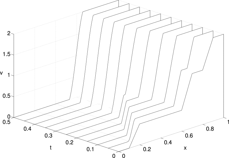
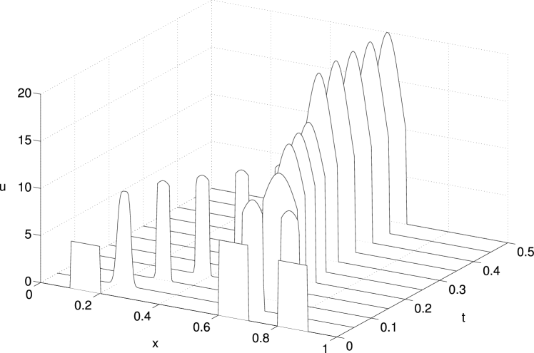
Figure 1. Example 1: Numerical approximation of $v$ (top) and corresponding approximation of $u$ (bottom), obtained via (4.3) with $\Delta x=0.001$.

$\Delta x$	$e^{t_{1}}_{v}$	${}^{\mathrm{conv.}}_{\mathrm{rate}}$	$e^{t_{2}}_{v}$	${}^{\mathrm{conv.}}_{\mathrm{rate}}$	$e^{t_{1}}_{u}$	${}^{\mathrm{conv.}}_{\mathrm{rate}}$	$e^{t_{2}}_{u}$	${}^{\mathrm{conv.}}_{\mathrm{rate}}$
0.020	0.239	-	0.317	-	0.915	-	0.695	-
0.010	0.133	0.845	0.146	1.122	0.513	0.834	0.442	0.655
0.005	0.061	1.135	0.069	1.070	0.246	1.062	0.200	1.144
0.004	0.048	1.018	0.054	1.090	0.181	1.369	0.164	0.891
0.002	0.021	1.168	0.024	1.161	0.082	1.150	0.073	1.163
0.001	0.008	1.360	0.009	1.399	0.036	1.167	0.032	1.200

Table 1. Example 1: Numerical error at $t_{1}=0.1$ and $t_{2}=0.25$.

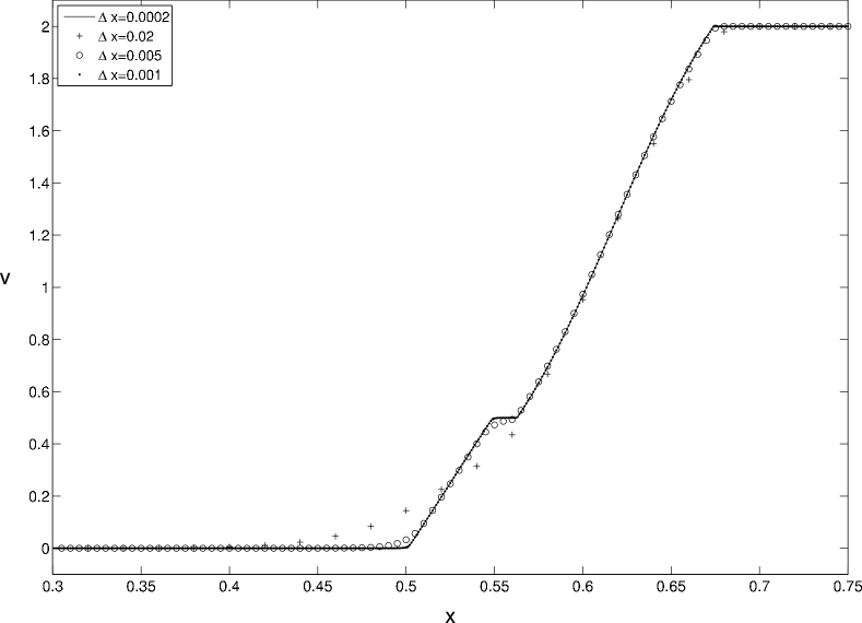
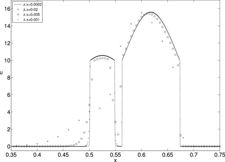
Figure 2. Example 1: Numerical approximation of $v$ (top) and $u$ (bottom) for several mesh sizes at $t=0.25$.

5.1. Example 1

In Example 1 we calculate the numerical solution of (1.1), (1.2) for $\Phi(v)=-(1-v)^{2}$ and the degenerating diffusion coefficient

$$A(u)=\begin{cases}0&\text{for $0\leq u\leq 10$,}\\ 0.1(u-10)&\text{for $u>10$.}\end{cases}$$

The initial datum is given by

$$u_{0}(x)=\begin{cases}5\quad\text{for $0.1\leq x\leq 0.2$,}\quad&7\quad\text{for $0.8\leq x\leq 0.9$,}\\ 8\quad\text{for $0.6\leq x\leq 0.7$,}&0\quad\text{otherwise.}\end{cases}$$

Note that $C_{0}=2$ in Example 1, where $C_{0}$ is defined in (1.11), and $v^{*}=C_{0}/2=1$, so that the function $\Phi$ corresponds to (1.12), where the constant of integration is $-1$, and that $u_{0}$ is chosen such that (1.8) is satisfied. Moreover, in our case $\Phi^{\prime\prime}(v)=-2<0$, and $\Phi(0)=\Phi(C_{0})=-1$. Nagai and Mimura [23] show that under these conditions, and for the integrated diffusion coefficient given by (1.16), the solution converges in time to a compactly supported, stationary travelling-wave solution, which represents the aggregated group of individuals and is defined by the time-independent version of (1.1).

In Figure 1 we show the numerical approximations for $v$ and $u$ for $0\leq t\leq 0.5$ and for $\Delta x=0.001$. As predicted, for each fixed time the data $\smash{\{v_{j}^{n}\}}$ are monotonically increasing, and the numerical solution for $u$ indeed displays the aggregation phenomenon, and terminates in a stationary profile, even though the assumptions on $A(\cdot)$ stated in [23] are not satisfied here. This supports the conjecture that a similar travelling wave analysis can also be conducted in the present strongly degenerate case, to which we will come back in a separate paper.

In Table 1 we show the error at $t_{1}=0.1$ and $t_{2}=0.25$ in the $L^{1}$ norm for $u$ (denoted as $\smash{e^{t_{i}}_{u}}$, $i=1,2$) and in the $L^{\infty}$ norm for $v$ (denoted as $\smash{e^{t_{i}}_{v}}$, $i=1,2$), where we take as a reference the solution calculated with $\Delta x=0.0002$. We find an experimental rate of convergence in both cases greater than one. For small $\Delta x$ this behavior is possibly related to the proximity of the reference solution. One should expect a real order of convergence at most one since the $v$-scheme is monotone.

In Figure 2 we compare the numerical approximations for $v$ and $a$ for different mesh sizes at the simulated time $t=0.25$.

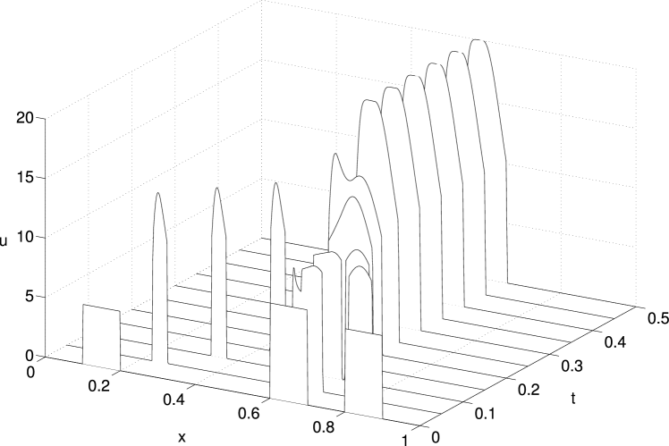
Figure 3. Example 2: Numerical approximation of $u$, obtained via (4.3) with $\Delta x=0.001$.

5.2. Example 2

This example represents a slight modification of Example 1, namely we choose $A(\cdot)$ and $u_{0}$ as in Example 1 but use

$$\Phi(v)=\begin{cases}-(1-v)^{8}&\textrm{for $0\leq v\leq 1$,}\\ -(1-v)^{2}&\textrm{for $v>1$.}\end{cases}$$

The function $\Phi$ has its maximum in $v^{*}=1$ and satisfies $\Phi(0)=\Phi(C_{0})$, as in Example 1, so we expect to see an aggregation phenomenon and the formation of a stationary travelling wave, even though here $\Phi$ is not symmetric with respect to $v^{*}$. In Figure 3 we show the numerical approximation of $u$ for $0\leq t\leq 0.5$ and $\Delta x=0.001$. The solution behavior is similar to that of Example 1, but the shapes of the “peaks” are slightly different, in particular the final “peak” is asymmetric.

5.3. Example 3

We now choose $\Phi$ and $u_{0}$ as in Example 1, but define $A(\cdot)$ by

$$A(u)=\begin{cases}0.05u&\text{for $0\leq u\leq 5$,}\\ 0.25&\text{for $5<u\leq 10$,}\\ 0.05u-0.25&\text{for $u>10$.}\end{cases}$$

Figure 4 shows the results for $\Delta x=0.001$ and $t\in[0,0.5]$. Again, a stationary single-peak solution is forming, including a jump between $u=5$ and $u=10$, in agreement with the flatness of $A(u)$ for $u\in[5,10]$. Table 2 shows the error of the approximations of $v$ and $u$ at $t_{1}=0.1$ and $t_{2}=0.25$. The reference solution has been calculated with $\Delta x=0.0002$. The observed rate of convergence is again one.

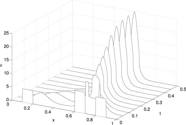
Figure 4. Example 3: Numerical approximation of $u$, obtained via (4.3) for $\Delta x=0.001$.

$\Delta x$	$e^{t_{1}}_{v}$	${}^{\mathrm{conv.}}_{\mathrm{rate}}$	$e^{t_{2}}_{v}$	${}^{\mathrm{conv.}}_{\mathrm{rate}}$	$e^{t_{1}}_{u}$	${}^{\mathrm{conv.}}_{\mathrm{rate}}$	$e^{t_{2}}_{u}$	${}^{\mathrm{conv.}}_{\mathrm{rate}}$
0.020	0.167	-	0.330	-	0.329	-	0.297	-
0.010	0.083	1.010	0.166	0.994	0.185	0.834	0.161	0.884
0.005	0.039	1.099	0.079	1.066	0.105	0.812	0.086	0.912
0.004	0.031	0.932	0.062	1.097	0.089	0.733	0.064	1.322
0.002	0.014	1.195	0.028	1.170	0.043	1.060	0.034	0.886
0.001	0.006	1.165	0.010	1.414	0.021	1.056	0.016	1.115

Table 2. Example 3: Numerical error for $u$ and $v$ at $t_{1}=0.1$ and $t_{2}=0.25$.

5.4. Example 4

In this example we utilize a flux function with several extrema given by $\Phi(v)=-0.5(\cos(v\pi)+1)$ combined with the integrated diffusion coefficient

$$A(u)=\begin{cases}0&\text{for $0\leq u\leq 10$,}\\ 0.1(u-10)&\text{for $u>10$}\end{cases}$$

and the initial datum

$$u_{0}(x)=\begin{cases}10\quad\text{for $x\in[0.05,0.15]$,}&9\quad\text{for $x\in[0.6,0.7]$,}\\ 14\quad\text{for $x\in[0.3,0.5]$,}&8\quad\text{for $x\in[0.9,1]$,}\\ &0\quad\text{otherwise.}\end{cases}$$

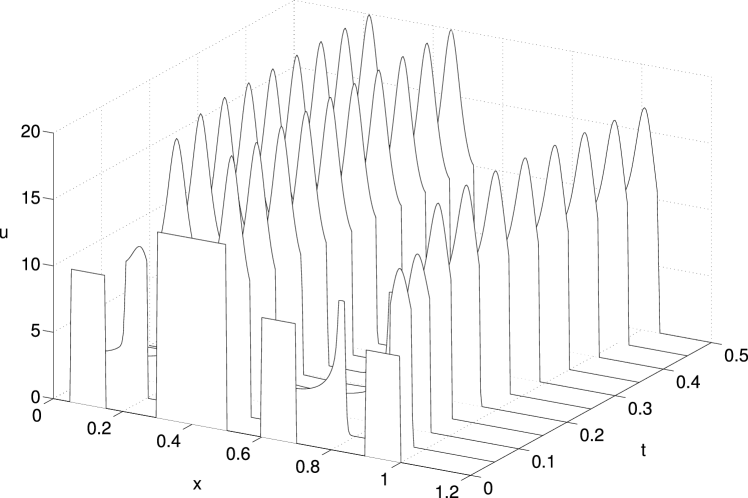
Figure 5. Example 4: Numerical approximation of $u$, obtained via (4.3) for $\Delta x=0.001$.

Figure 6. Example 4: Contour lines of the numerical approximation of $v$ for $\Delta x=0.001$.

The result is shown in Figure 5 for $\Delta x=0.001$. We observe the formation of three groups, but the third moves to the right “looking for more” mass since it is not a full state, in the sense of the Nagai and Mimura [23] condition for the formation of stationary travelling waves. In addition to Figure 5 we show in Figure 6 a contour plot of the numerical approximation of $v$ for this example. The contour lines of $v$ correspond to trajectories of “individuals”. Table 3 shows the error for $v$ and $u$ taking as a reference the solution calculated with $\Delta x=0.0002$. We again find the order of convergence predicted for monotone schemes.

$\Delta x$	$e^{t_{1}}_{v}$	${}^{\mathrm{conv.}}_{\mathrm{rate}}$	$e^{t_{2}}_{v}$	${}^{\mathrm{conv.}}_{\mathrm{rate}}$	$e^{t_{1}}_{u}$	${}^{\mathrm{conv.}}_{\mathrm{rate}}$	$e^{t_{2}}_{u}$	${}^{\mathrm{conv.}}_{\mathrm{rate}}$
0.020	0.361	-	0.381	-	1.420	-	1.244	-
0.010	0.189	0.933	0.201	0.923	0.892	0.671	0.709	0.811
0.005	0.095	0.992	0.101	0.994	0.509	0.809	0.356	0.993
0.004	0.080	0.771	0.080	1.048	0.398	1.101	0.262	1.374
0.002	0.042	0.939	0.040	0.981	0.216	0.883	0.145	0.857
0.001	0.019	1.130	0.020	1.000	0.104	1.047	0.072	1.000

Table 3. Example 4: Numerical error for $u$ and $v$ at $t_{1}=0.1$ and $t_{2}=0.25$.

5.5. Example 5

Here we calculate the numerical approximation of $u$ for $A(\cdot)$ as in Example 4, but with $\Phi$ and $u_{0}$ given by the respective equations

$$\Phi(v)=\begin{cases}-0.5(\cos(v\pi)+1)&\text{for $0\leq v\leq 2$,}\\ (v-2)^{2}-1&\text{for $v>2$,}\end{cases}$$

$$u_{0}(x)=\begin{cases}14\quad\text{for $x\in[0.15,0.3]$,}&18\quad\text{for $x\in[0.8,0.95]$,}\\ 17\quad\text{for $x\in[0.6,0.7]$,}&0\;\,\quad\text{otherwise.}\end{cases}$$

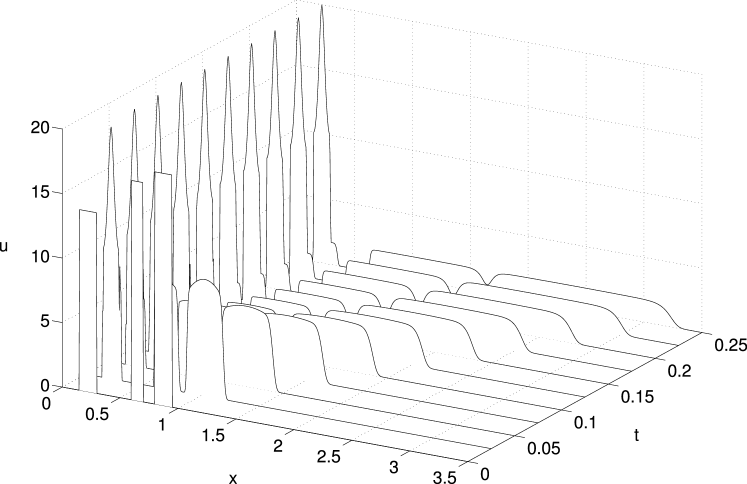
Figure 7. Example 5: Numerical approximation of $u$, obtained via (4.3) for $\Delta x=0.001$.

In Figure 7 we show the result for $\Delta x=0.001$. We see that the spare mass (i.e. the mass that can not get in the first group) “dilutes” to the right.

5.6. Example 6

We consider now the same initial data and parabolic term $A(\cdot)$ as in Example 1, but employ a function $\Phi$ with several extrema given by $\Phi(v)=-0.5\left(\cos(2\pi v)+1\right)$. Accordingly with the results of Example 1 we expect a steady state consisting of two traveling waves since $\Phi(0)=\Phi(C_{0})$. Figure 8 shows the numerical result for $u$ for $\Delta x=0.001$, which confirm our claim.

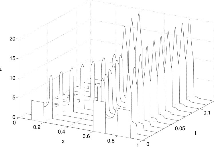
Figure 8. Example 6: Numerical approximation of $u$, obtained via (4.3) for $\Delta x=0.001$.

References

- [1] W. Alt. Degenerate diffusion equations with drift functionals modelling aggregation. Nonlin. Anal. TMA, 9:811–836, 1985.
- [2] A.L. Bertozzi, J.A. Carrillo and T. Laurent. Blow-up in multidimensional aggregation equations with mildly singular interaction kernels. Nonlinearity, 22:683–710, 2009.
- [3] A.L. Bertozzi and T. Laurent. Finite-time blow-up of solutions of an aggregation equation in . Comm. Math. Phys., 274:717–735, 2007.
- [4] M. Bodnar and J.J.L. Velazquez. An integro-differential equation arising as a limit of individual cell-based models. J. Differential Equations, 222:341–380, 2006.
- [5] M. Burger, V. Capasso, and D. Morale. On an aggregation model with long and short range interactions. Nonlin. Anal. Real World Appl., 8:939–958, 2007.
- [6] J.A. Carrillo, M. Di Francesco, A. Figalli, T. Laurent, and D. Slepcev. Global-in-time weak measure solutions and finite-time aggregation for nonlocal interaction equations. Duke Math. J., to appear.
- [7] A. Chertock, A. Kurganov, and P. Rosenau. On degenerate saturated-diffusion equations with convection. Nonlinearity, 18:609–630, 2005.
- [8] J.I. Diaz, T. Nagai, and S.I. Shmarev. On the interfaces in a nonlocal quasilinear degenerate equation arising in population dynamics. Japan J. Indust. Appl. Math., 13:385–415, 1996.
- [9] B. Engquist and S. Osher. One-sided difference approximations for nonlinear conservation laws. Math. Comp. 36:321–351, 1981.
- [10] S. Evje and K.H. Karlsen. Monotone difference approximations of solutions to degenerate convection-diffusion equations. SIAM J. Numer. Anal., 37:1838–1860, 2006.
- [11] S. Evje and K.H. Karlsen. Discrete approximations of solutions to doubly degenerate parabolic equations. Numer. Math., 86:377–417, 2000.
- [12] G.-Q. Chen and K. H. Karlsen. Quasilinear anisotropic degenerate parabolic equations with time-space dependent diffusion coefficients. Commun. Pure Appl. Anal., 4:241–266, 2005.
- [13] K.H. Karlsen and N.H. Risebro. Convergence of finite difference schemes for viscous and inviscid conservation laws with rough coefficients. M2AN Math. Model. Numer. Anal., 35:239–269, 2001.
- [14] K.H. Karlsen and N.H. Risebro. On the uniqueness and stability of entropy solutions for nonlinear degenerate parabolic equations with rough coefficients. Discr. Contin. Dyn. Syst., 9:1081–1104, 2003.
- [15] K.H. Karlsen, N.H. Risebro, and J.D. Towers. stability for entropy solutions of nonlinear degenerate parabolic convection-diffusion equations with discontinuous coefficients. Skr. K. Nor. Vid. Selsk., 3 (2003), pp. 1 -49.
- [16] D. Li and J. Rodrigo. Finite-time singularities of an aggregation equation in with fractional dissipation. Commun. Math. Phys., 287:687–703, 2009.
- [17] D. Li and J. Rodrigo. Refined blowup criteria and nonsymmetric blowup of an aggregation equation. Adv. in Math., 220:1717–1738, 2009.
- [18] D. Li and X. Zhang. On a nonlocal aggregation model with nonlinear diffusion. Discr. Cont. Dyn. Syst., 27:301–323, 2010.
- [19] A. Mogilner, L. Edelstein-Keshet, L. Bent, and A. Spiros. Mutual interactions, potentials, and individual distance in a social aggregation. J. Math. Biol., 47: 353–389, 2003.
- [20] D. Morale, V. Capasso, and K. Oelschläger. An interacting particle system modelling aggregation behavior: from individuals to populations. J. Math. Biol., 50:49–66, 2005.
- [21] T. Nagai. Some nonlinear degenerate diffusion equations with a nonlocally convective term in ecology. Hiroshima Math. J., 13:165–202, 1983.
- [22] T. Nagai and M. Mimura. Some nonlinear degenerate diffusion equations related to population dynamics. J. Math. Soc. Japan, 35:539–562, 1983.
- [23] T. Nagai and M. Mimura. Asymptotic behavior for a nonlinear degenerate diffusion equation in population dynamics. SIAM J. Appl. Math., 43:449–464, 1983.
- [24] T. Nagai and M. Mimura. Asymptotic behavior of the interfaces to a nonlinear degenerate diffusion equation in population dynamics. Japan J. Appl. Math., 3:129–161, 1986.
- [25] C.M. Topaz, A.L. Bertozzi, and M.A. Lewis. A nonlocal continuum model for biological aggregation. Bull. Math. Biol., 68:1601–1623, 2006.