Density matrix expansion for the MDI interaction

Abstract

By assuming that the isospin- and momentum-dependent MDI interaction has a form similar to the Gogny-like effective two-body interaction with a Yukawa finite-range term and the momentum dependence only originates from the finite-range exchange interaction, we determine its parameters by comparing the predicted potential energy density functional in uniform nuclear matter with what has been usually given and used extensively in transport models for studying isospin effects in intermediate-energy heavy-ion collisions as well as in investigating the properties of hot asymmetric nuclear matter and neutron star matter. We then use the density matrix expansion to derive from the resulting finite-range exchange interaction an effective Skyrme-like zero-range interaction with density-dependent parameters. As an application, we study the transition density and pressure at the inner edge of neutron star crusts using the stability conditions derived from the linearized Vlasov equation for the neutron star matter.

I Introduction

One of the phenomenological nucleon-nucleon interactions that have been extensively used in transport models to study heavy-ion collisions is the isospin- and momentum-dependent MDI interaction Das03 . By using this interaction in the isospin-dependent Boltzmann-Uhling-Uhlenbeck (IBUU) transport model, an extensive amount of works have been carried out to study various isospin sensitive observables in intermediate-energy heavy-ion collisions (for recent reviews see Refs. Chen07 ; LCK08 ). From comparisons of the isospin diffusion data from NSCL-MSU for ¹²⁴Sn+¹¹²Sn reactions at $E=50$ MeV/nucleon Tsa04 with results from the IBUU model, a relatively stringent constraint on the density dependence of the nuclear symmetry energy at subsaturation densities has been obtained Che05a ; LiBA05 . The resulting symmetry energy has further been used to impose constraints on both the parameters in the Skyrme effective interactions and the neutron skin thickness of heavy nuclei Che05 . The MDI interaction with the constrained isospin dependence has also been used to study the properties of hot asymmetric nuclear matter Xu08 as well as those of neutron stars Steiner06 ; Krastev08a ; Krastev08b ; Wen09 ; Newton09 ; bali08 , including the transition density which separates their liquid core from their inner crust XCLM09 . New constraints on the masses and radii of neutron stars were then obtained from comparing the resulting crustal fraction of the moment of inertia of neutron stars with that of the Vela pulsar extracted from its glitches XCLM09 .

Although the momentum-dependent nuclear mean-field potential or the energy density functional of uniform nuclear matter was used in the above mentioned applications of the MDI interaction, the explicit form of the MDI interaction has never been given in the literatures. It was, however, implicitly mentioned Das03 ; Gal90 that this momentum-dependent nucleon mean-field potential was constructed according to a Gogny-like interaction Gog80 consisting of a zero-range Skyrme-like interaction Vau72 and a finite-range Yukawa interaction as in the MDYI interaction Gal90 . Similar to the Gogny interaction, the momentum dependence in the nucleon mean-field potential from the MDI interaction is then from the contribution of the finite-range Yukawa interaction to the exchange energy density of uniform nuclear matter. The effect of the finite-range part of the MDI interaction in nonuniform nuclear matter was in previous applications either neglected or inconsistently included by using the average density-gradient terms from the phenomenological Skyrme interactions. From comparing the potential energy density functional obtained from above assumed interaction with that used in previous applications of the MDI interaction, we are able to find unique relations among the parameters of this interaction and those used in the potential energy density functional for uniform nuclear matter.

As a first step to facility the consistent application of the finite-range MDI interaction, it is of interest to derive an effective zero-range interaction with density-dependent parameters using the density matrix expansion first introduced in Ref. Neg72 . As shown in Ref. Spr75 for other finite-range interactions, corresponding zero-range interactions derived from the density matrix expansion reproduce reasonably well in the self-consistent Hartree-Fock approach the binding energies and radii of nuclei obtained with the original interactions, particularly if the density matrix expansion is only used for the exchange energy from the finite-range interaction Neg72 ; Spr75 . In the present paper, we carry out such a study as an attempt to include consistently the effect due to the finite-range part of the MDI interaction. As an application, we use the resulting interaction to study the transition density and pressure in neutron stars and compare the results with those from previous studies using the MDI interaction but with inconsistent density-gradient coefficients XCLM09 ; Xu10 .

This paper is organized as follows. In Sec. II, we review the isospin- and momentum-dependent MDI interaction and determine its underlying nucleon-nucleon (NN) interaction by fitting the energy density functional used in previous applications of the MDI interaction. In Sec. III, the density matrix expansion is then used to derive from the finite-range exchange interaction a zero-range effective interaction with density-dependent parameters. The application of the resulting interaction to study the transition density and pressure at the inner edge of neutron star crusts is given in Sec. IV, using the stability conditions that are derived from the linearized Vlasov equation for the neutron star matter. Finally, the summary is given in Sec. V. For details on the determination of the underlying nucleon-nucleon interaction potential in the MDI interaction and the application of the density matrix expansion to the exchange energy of nuclear matter, they are given in Appendices A and B, respectively.

II The MDI interaction

In applications of the momentum-dependent MDI interaction for studying isospin effects in intermediate-energy heavy-ion collisions as well as the properties of hot asymmetric nuclear matter and neutron star matter, one usually uses following potential energy density

$$H(\rho,\delta) = \frac{A_{1}}{2\rho_{0}}\rho^{2}+\frac{A_{2}}{2\rho_{0}}\rho^{2}\delta^{2}+\frac{B}{\sigma+1}\frac{\rho^{\sigma+1}}{\rho_{0}^{\sigma}}(1-x\delta^{2})$$

$$+ \frac{1}{\rho_{0}}\sum_{\tau,\tau^{\prime}}C_{\tau,\tau^{\prime}}\int\int d^{3}pd^{3}p^{\prime}\frac{f_{\tau}(\vec{r},\vec{p})f_{\tau^{\prime}}(\vec{r},\vec{p}^{\prime})}{1+(\vec{p}-\vec{p}^{\prime})^{2}/\Lambda^{2}}$$

for infinite nuclear matter of density $\rho$ and isospin asymmetry $\delta=(\rho_{n}-\rho_{p})/\rho$, with $\rho_{n}$ and $\rho_{p}$ being, respectively, the neutron and proton densities. In the above, $\tau(\tau^{\prime})$ is the nucleon isospin; $f_{\tau}(\vec{r},\vec{p})$ is the nucleon phase-space distribution function at position $\vec{r}$; and $\rho_{0}=0.16$ fm^-3 is the saturation density of normal nuclear matter. Values of the parameters $A_{1}=(A_{l}+A_{u})/2$, $A_{2}=(A_{l}-A_{u})/2$, $B$, $\sigma$, $\Lambda$, $C_{l}=C_{\tau,\tau}$ and $C_{u}=C_{\tau,-\tau}$ can be found in Refs. Das03 ; Che05a . For symmetric nuclear matter, this interaction gives a binding energy of $-16$ MeV per nucleon and an incompressibility $K_{0}$ of $212$ MeV at saturation density.

The parameter $x$ in Eq. (LABEL:MDIV) is used to model the density dependence of the symmetry energy. Based on analyses of the isospin diffusion in intermediate-energy heavy-ion collisions and the neutron skin thickness of heavy nuclei Tsa04 ; Che05a ; LiBA05 , the slope parameter $L=3\rho_{0}(\partial E_{\rm sym}(\rho)/\partial\rho)_{\rho=\rho_{0}}$ of the symmetry energy has been constrained to $L=86\pm 25$ MeV, which corresponds to $-1<x<0$. More recent analyses of experimental data on isospin diffusion, double $n/p$ ratio, and neutron skin thickness favor, however, a softer symmetry energy of $L=58\pm 18$ MeV Tsa09 ; She10 ; Che10 .

The momentum dependence in the MDI interaction can come from a number of different origins. Besides the finite-range exchange term in the nucleon-nucleon interaction, the intrinsic momentum dependence in the nucleon-nucleon interaction and the effects of short-range nucleon-nucleon correlations Pan05 can also contribute to its momentum dependence. For simplicity, we assume in the present study that all of the momentum dependence in the MDI interaction comes from the finite-range exchange term. In this case, the explicit form for the MDI interaction can be obtained from the energy density given in Eq. (LABEL:MDIV) by assuming that the interaction potential between two nucleons located at $\vec{r}_{1}$ and $\vec{r}_{2}$ has a form similar to the Gogny interaction Gog80 ; Das03 but with its Gaussian form in the finite-range term replaced by a Yukawa form, that is

$$v(\vec{r}_{1},\vec{r}_{2}) = \frac{1}{6}t_{3}(1+x_{3}P_{\sigma})\rho^{\alpha}\left(\frac{\vec{r}_{1}+\vec{r}_{2}}{2}\right)\delta(\vec{r}_{1}-\vec{r}_{2})$$

$$+ (W+BP_{\sigma}-HP_{\tau}-MP_{\sigma}P_{\tau})\frac{e^{-\mu|\vec{r}_{1}-\vec{r}_{2}}|}{|\vec{r}_{1}-\vec{r}_{2}|}.$$

In the above equation, the first term is the density-dependent zero-range interaction which can be considered as an effective three-body interaction, whereas the second term is the density-independent finite-range interaction. In terms of this nucleon-nucleon interaction, the total potential energy of a nuclear system can be calculated from

$$E=\frac{1}{2}\sum_{i,j}<ij|v(1-P_{r}P_{\sigma}P_{\tau})|ij>,$$ (3)

where

$$|i>=|i_{r}i_{\sigma}i_{\tau}>$$ (4)

is the quantum state of nucleon $i$ with the spatial state $i_{r}$, the spin state $i_{\sigma}$, and the isospin state $i_{\tau}$, and $P_{r}$, $P_{\sigma}$ and $P_{\tau}$ are, respectively, the space, spin and isospin exchange operators.

As shown in Appendix A, where the detailed derivation of Eq. (LABEL:MDIV) from Eq. (LABEL:MDIv) is given, the first and second terms in Eq. (LABEL:MDIV) come from the direct contribution (the first term of Eq. (3)) of the finite-range term in the NN interaction. The third term in Eq. (LABEL:MDIV) is simply from the contribution of the zero-range term. Although different density-dependent zero-range terms can lead to different symmetry energies/potentials XuC10 , we use in the present study the one in the standard Skyrme interaction Cha97 . The momentum-dependent terms in Eq. (LABEL:MDIV) come from the exchange contribution (the second term of Eq. (3)) of the finite-range interaction. Comparing the resulting energy density functional with Eq. (LABEL:MDIV) leads to following unique relations between the 8 parameters in the NN interaction and those in the energy density functional of Eq. (LABEL:MDIV):

$$t_{3} = \frac{16B}{(\sigma+1)\rho_{0}^{\sigma}},$$ (5)

$$x_{3} = \frac{3x-1}{2},$$ (6)

$$\alpha = \sigma-1,$$ (7)

$$\mu = \Lambda,$$ (8)

$$W = \frac{\Lambda^{2}}{3\pi\rho_{0}}(A_{1}-A_{2}+C_{l}-C_{u}),$$ (9)

$$B = \frac{\Lambda^{2}}{6\pi\rho_{0}}(-A_{1}+A_{2}-4C_{l}+4C_{u}),$$ (10)

$$H = \frac{\Lambda^{2}}{3\pi\rho_{0}}(-2A_{2}-C_{u}),$$ (11)

$$M = \frac{\Lambda^{2}}{3\pi\rho_{0}}(A_{2}+2C_{u}).$$ (12)

It is seen that the symmetry energy parameter $x$ is related to the coefficient of the spin-exchange term in the density-dependent zero-range interaction, whereas the width $\Lambda$ in the momentum dependence is related to the range of the finite-range interaction.

In the original MDI interaction Das03 , the symmetry energy parameter $x$ can only have the value of $0$ or $1$. To get a larger range of density dependence for the symmetry energy while fixing the value of $E_{\rm sym}(\rho_{0})=30.5$ MeV, the parameters $A_{l}$ and $A_{u}$ have been expressed as Che05a

$$A_{l}=-120.57+x\frac{2B}{\sigma+1},~{}A_{u}=-95.98-x\frac{2B}{\sigma+1},$$ (13)

which results in the $x$ dependence of $A_{2}$. Therefore, with this constraint the $x$ dependence also appears in the finite-range direct interaction.

III The density Matrix Expansion

Although the contribution of a finite-range interaction to the direct energy density of nuclear matter can be treated exactly, it is numerically challenging to evaluate its contribution to the exchange energy density. The latter can be, however, approximated by that from a Skyrme-like zero-range interaction using the density-matrix expansion of Ref. Neg72 . As shown in Appendix B, the resulting exchange energy density from the finite-range interaction at position $\vec{r}$ in a nuclear system can be expressed in terms of densities $\rho_{n}$ and $\rho_{p}$ as well as kinetic energy densities $\tau_{n}$ and $\tau_{p}$ as

$$H_{SL}^{E}(\vec{r}) = A[\rho_{n}(\vec{r}),\rho_{p}(\vec{r})]$$ (14)

$$+ B[\rho_{n}(\vec{r}),\rho_{p}(\vec{r})]\tau_{n}(\vec{r})+B[\rho_{p}(\vec{r}),\rho_{n}(\vec{r})]\tau_{p}(\vec{r})$$

$$+ C[\rho_{n}(\vec{r}),\rho_{p}(\vec{r})]|\nabla\rho_{n}(\vec{r})|^{2}$$

$$+ C[\rho_{p}(\vec{r}),\rho_{n}(\vec{r})]|\nabla\rho_{p}(\vec{r})|^{2}$$

$$+ D[\rho_{n}(\vec{r}),\rho_{p}(\vec{r})]\nabla\rho_{n}(\vec{r})\cdot\nabla\rho_{p}(\vec{r}),$$

where

$$A(\rho_{n},\rho_{p}) = V_{NM}(\rho_{n},\rho_{p})-\frac{3}{5}(3\pi^{2})^{2/3}[\rho_{n}^{5/3}B(\rho_{n},\rho_{p})$$ (15)

$$+ \rho_{p}^{5/3}B(\rho_{p},\rho_{n})],$$

$$B(\rho_{n},\rho_{p}) = -2[\rho_{n}V^{L}(\rho_{n})+\rho_{p}V^{U}(\rho_{p},\rho_{n})],$$ (16)

$$C(\rho_{n},\rho_{p}) = -\frac{\partial F(\rho_{n},\rho_{p})}{\partial\rho_{n}},$$ (17)

$$D(\rho_{n},\rho_{p}) = -\frac{\partial F(\rho_{n},\rho_{p})}{\partial\rho_{p}}-\frac{\partial F(\rho_{p},\rho_{n})}{\partial\rho_{n}}.$$

In above equations, $V_{NM}(\rho_{n},\rho_{p})$ is the potential energy density of infinite nuclear matter from the finite-range exchange interaction (i.e. the momentum-dependent terms in Eq. (LABEL:MDIV)) and is given by

$$V_{NM}(\rho_{n},\rho_{p}) = \rho_{n}^{2}V_{NM}^{L}(\rho_{n})+\rho_{p}^{2}V_{NM}^{L}(\rho_{p})$$ (19)

$$+ 2\rho_{n}\rho_{p}V_{NM}^{U}(\rho_{n},\rho_{p}),$$

with

$$V_{NM}^{L}(\rho_{\tau}) = \frac{1}{2}\left(M+\frac{H}{2}-B-\frac{W}{2}\right)$$ (20)

$$\times \int d^{3}s\rho_{SL}^{2}(k_{\tau}s)\frac{e^{-\mu s}}{s},$$

$$V_{NM}^{U}\left(\rho_{\tau},\rho_{\tau^{\prime}}\right) = \frac{1}{2}\left(M+\frac{H}{2}\right)$$ (21)

$$\times \int d^{3}s\rho_{SL}(k_{\tau}s)\rho_{SL}(k_{\tau^{\prime}}s)\frac{e^{-\mu s}}{s}.$$

Other terms are defined as

$$V^{L}(\rho_{\tau}) = \frac{1}{2}\left(M+\frac{H}{2}-B-\frac{W}{2}\right)$$ (22)

$$\times \int d^{3}ss^{2}\rho_{SL}(k_{\tau}s)g(k_{\tau}s)\frac{e^{-\mu s}}{s},$$

$$V^{U}(\rho_{\tau},\rho_{\tau^{\prime}}) = \frac{1}{2}\left(M+\frac{H}{2}\right)$$ (23)

$$\times \int d^{3}ss^{2}\rho_{SL}(k_{\tau}s)g(k_{\tau^{\prime}}s)\frac{e^{-\mu s}}{s},$$

where

$$\rho_{SL}(k_{\tau}s) = \frac{3}{k_{\tau}s}j_{1}(k_{\tau}s),$$ (24)

$$g(k_{\tau}s) = \frac{35}{2(k_{\tau}s)^{3}}j_{3}(k_{\tau}s),$$ (25)

with $j_{1}$ and $j_{3}$ being, respectively, the first- and third-order spherical bessel functions and $k_{\tau}=(3\pi^{2}\rho_{\tau})^{1/3}$ is the Fermi momentum. For the function $F(\rho_{n},\rho_{p})$, it is defined as

$$F(\rho_{n},\rho_{p})=\frac{1}{2}V^{L}(\rho_{n})\rho_{n}+\frac{1}{2}V^{U}(\rho_{p},\rho_{n})\rho_{p}.$$ (26)

In Fig. 1, we show the dependence of $A(\rho_{n},\rho_{p})$, $B(\rho_{n},\rho_{p})$, $C(\rho_{n},\rho_{p})$ and $D(\rho_{n},\rho_{p})$ on $\rho_{n}$ and $\rho_{p}$ at subsaturation densities. It is seen that $A(\rho_{n},\rho_{p})$ and $D(\rho_{n},\rho_{p})$ are symmetric in $\rho_{n}$ and $\rho_{p}$, while $B(\rho_{n},\rho_{p})$ and $C(\rho_{n},\rho_{p})$ are not. Furthermore, the density dependence of $B(\rho_{n},\rho_{p})$, $C(\rho_{n},\rho_{p})$ and $D(\rho_{n},\rho_{p})$ are strong at low densities but weak near the saturation density. As these functions are from the exchange contribution of the finite-range interaction, they are independent of $x$.

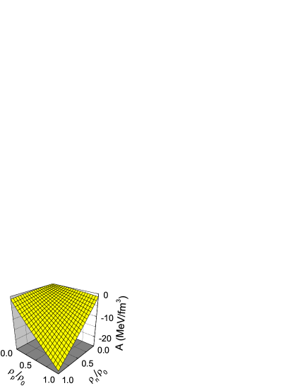
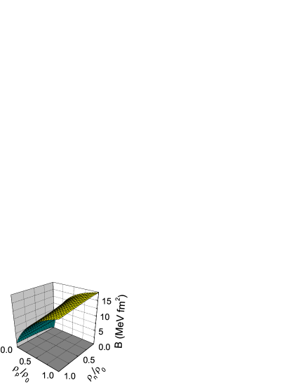
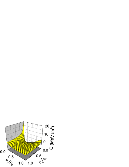
Figure 1: (Color online) Dependence of $A(\rho_{n},\rho_{p})$, $B(\rho_{n},\rho_{p})$, $C(\rho_{n},\rho_{p})$ and $D(\rho_{n},\rho_{p})$ on $\rho_{n}$ and $\rho_{p}$ at subsaturation densities.

IV Application: transition density and pressure in neutron stars

The explicit form of the finite-range NN interaction and the Skyrme-like zero-range interaction with density-dependent parameters derived in previous sections make it convenient to use the MDI interaction for a wider range of studies. In this Section, we discuss its application in studying the transition density and pressure at the inner edge of neutron star crusts based on the stability conditions that are derived from the linearized Vlasov equation for the neutron star matter.

IV.1 The single-particle Hamiltonian

The single-particle Hamiltonian for a nucleon can be obtained from minimizing the total energy of a nuclear system with respect to its wave function. For a neutron, it is given by

$$h_{n} = -\nabla\cdot\left(\frac{\hbar^{2}}{2m_{n}^{\star}}\nabla\right)+U_{n}(\rho_{n},\rho_{p})$$ (27)

with the neutron effective mass

$$\frac{\hbar^{2}}{2m_{n}^{\star}}=\frac{\hbar^{2}}{2m}+B(\rho_{n},\rho_{p}),$$ (28)

and the potential

$$U_{n}(\rho_{n},\rho_{p})=U_{n}^{\rho}(\rho_{n},\rho_{p})+U_{n}^{D}(\rho_{n},\rho_{p})+U_{n}^{E}(\rho_{n},\rho_{p}),$$ (29)

where

$$U_{n}^{\rho}(\rho_{n},\rho_{p})=\frac{\partial H_{0}(\rho_{n},\rho_{p})}{\partial\rho_{n}}$$ (30)

is the contribution from the the zero-range interaction with

$$H_{0}(\rho_{n},\rho_{p})=\frac{1}{24}t_{3}\rho^{\alpha}[(2+x_{3})\rho^{2}-(2x_{3}+1)(\rho_{n}^{2}+\rho_{p}^{2})]$$ (31)

being the corresponding energy density, and

$$U_{n}^{D}(\rho_{n},\rho_{p}) = (W+\frac{B}{2}-H-\frac{M}{2})\int d^{3}r^{\prime}\rho_{n}(\vec{r}^{\prime})\frac{e^{-\mu|\vec{r}-\vec{r}^{\prime}}|}{|\vec{r}-\vec{r}^{\prime}|}$$ (32)

$$+ (W+\frac{B}{2})\int d^{3}r^{\prime}\rho_{p}(\vec{r}^{\prime})\frac{e^{-\mu|\vec{r}-\vec{r}^{\prime}}|}{|\vec{r}-\vec{r}^{\prime}|},$$

$$U_{n}^{E}(\rho_{n},\rho_{p}) = \frac{\partial A(\rho_{n},\rho_{p})}{\partial\rho_{n}}+\frac{\partial B(\rho_{n},\rho_{p})}{\partial\rho_{n}}\tau_{n}$$ (33)

$$+ \frac{\partial B(\rho_{p},\rho_{n})}{\partial\rho_{n}}\tau_{p}-\frac{\partial C(\rho_{n},\rho_{p})}{\partial\rho_{n}}(\nabla\rho_{n})^{2}$$

$$+ \left(\frac{\partial C(\rho_{p},\rho_{n})}{\partial\rho_{n}}-\frac{\partial D(\rho_{n},\rho_{p})}{\partial\rho_{p}}\right)(\nabla\rho_{p})^{2}$$

$$- 2\frac{\partial C(\rho_{n},\rho_{p})}{\partial\rho_{p}}\nabla\rho_{n}\cdot\nabla\rho_{p}-2C(\rho_{n},\rho_{p})\nabla^{2}\rho_{n}$$

$$- D(\rho_{n},\rho_{p})\nabla^{2}\rho_{p}$$

are the direct and exchange contributions from the finite-range interaction, respectively. Expressing the kinetic energy density in the exchange potential in terms of the density via the extended Thomas-Fermi (ETF) approximation Jen76 ; Bra85

$$\tau_{q}=a\rho_{q}^{5/3}+b\frac{(\nabla\rho_{q})^{2}}{\rho_{q}}+c\nabla^{2}\rho_{q},~{}q=n,p,$$ (34)

where $a=\frac{3}{5}(3\pi^{2})^{2/3}$, $b=1/36$ and $c=1/3$, the neutron potential can then be written as

$$U_{n} = U_{n}^{0}+U_{n}^{D}+U_{n}^{\nabla},$$ (35)

where

$$U_{n}^{0}(\rho_{n},\rho_{p}) = U_{n}^{\rho}(\rho_{n},\rho_{p})+\frac{\partial A(\rho_{n},\rho_{p})}{\partial\rho_{n}}$$ (36)

$$+ a\frac{\partial B(\rho_{n},\rho_{p})}{\partial\rho_{n}}\rho_{n}^{5/3}+a\frac{\partial B(\rho_{p},\rho_{n})}{\partial\rho_{n}}\rho_{p}^{5/3},$$

$$U_{n}^{\nabla}(\rho_{n},\rho_{p}) = G_{n}^{nn1}(\nabla\rho_{n})^{2}+G_{n}^{pp1}(\nabla\rho_{p})^{2}$$

$$+ G_{n}^{np}\nabla\rho_{n}\cdot\nabla\rho_{p}+G_{n}^{nn2}\nabla^{2}\rho_{n}+G_{n}^{pp2}\nabla^{2}\rho_{p},$$

with

$$G_{n}^{nn1}(\rho_{n},\rho_{p}) = -\frac{\partial C(\rho_{n},\rho_{p})}{\partial\rho_{n}}+\frac{b}{\rho_{n}}\frac{\partial B(\rho_{n},\rho_{p})}{\partial\rho_{n}},$$ (38)

$$G_{n}^{pp1}(\rho_{n},\rho_{p}) = \frac{\partial C(\rho_{p},\rho_{n})}{\partial\rho_{n}}-\frac{\partial D(\rho_{n},\rho_{p})}{\partial\rho_{p}}$$ (39)

$$+ \frac{b}{\rho_{p}}\frac{\partial B(\rho_{p},\rho_{n})}{\partial\rho_{n}},$$

$$G_{n}^{np}(\rho_{n},\rho_{p}) = -2\frac{\partial C(\rho_{n},\rho_{p})}{\partial\rho_{p}},$$ (40)

$$G_{n}^{nn2}(\rho_{n},\rho_{p}) = -2C(\rho_{n},\rho_{p})+c\frac{\partial B(\rho_{n},\rho_{p})}{\partial\rho_{n}},$$ (41)

$$G_{n}^{pp2}(\rho_{n},\rho_{p}) = -D(\rho_{n},\rho_{p})+c\frac{\partial B(\rho_{p},\rho_{n})}{\partial\rho_{n}}.$$ (42)

Similarly, the proton single-particle Hamiltonian is

$$h_{p}=h_{n}(n\leftrightarrow p)+U_{p}^{CD}+U_{p}^{CE},$$ (43)

where the first term $h_{n}(n\leftrightarrow p)$ is due to the nuclear interaction and is obtained from Eq. (27) by interchanging the neutron and proton symbols; the second term $U_{p}^{CD}$ is the direct Coulomb potential given by

$$U_{p}^{CD}=e^{2}\int\frac{\rho_{p}(\vec{r}^{\prime})-\rho_{e}(\vec{r}^{\prime})}{|\vec{r}-\vec{r}^{\prime}|}d^{3}r^{\prime};$$ (44)

and the last term $U_{p}^{CE}$ is the exchange Coulomb potential which in the first order of the density matrix expansion Neg72 is given by

$$U_{p}^{CE}=-e^{2}\left(\frac{3}{\pi}\right)^{1/3}\rho_{p}^{1/3}.$$ (45)

IV.2 The Vlasov equation for the neutron star matter

The Vlasov equation has been widely used in studying the collective density fluctuation and spinodal instability in nuclear matter (See Ref. Cho04 for a recent review). For a $\beta$-stable and charge neutral $npe$ matter, the Vlasov equation can be written as

$$\frac{\partial f_{q}(\vec{r},\vec{p},t)}{\partial t}+\vec{v}_{q}\cdot\nabla_{\vec{r}}f_{q}(\vec{r},\vec{p},t)-\nabla_{\vec{r}}U_{q}\cdot\nabla_{\vec{p}}f_{q}(\vec{r},\vec{p},t)=0$$ (46)

in terms of the Wigner function for particle type $q=n,p,e$

$$f_{q}(\vec{r},\vec{p},t) = \frac{1}{(2\pi)^{3}}\sum_{i}\int\phi_{qi}\left(\vec{r}-\frac{\vec{s}}{2},t\right)$$ (47)

$$\times \phi_{qi}^{\star}\left(\vec{r}+\frac{\vec{s}}{2},t\right)e^{i\vec{p}\cdot\vec{s}}d^{3}s,$$

where $\phi_{qi}$ is the wave function of i-th particle of type $q$. In Eq. (46), $\vec{v}_{q}=\vec{p}/{(m_{q}^{\star}}^{2}+p^{2})^{1/2}$ denotes the particle velocity and $m_{e}^{\star}=m_{e}$.

To study the density fluctuation due to a collective mode with frequency $\omega$ and wavevector $\vec{k}$ in the nuclear matter, we follow the standard procedure Cho04 by writing

$$f_{q}(\vec{r},\vec{p},t)=f_{q}^{0}(\vec{p})+\delta f_{q}(\vec{r},\vec{p},t)$$ (48)

with

$$\delta f_{q}(\vec{r},\vec{p},t)=\delta\tilde{f_{q}}(\vec{p})e^{-i\omega t+i\vec{k}\cdot\vec{r}}.$$ (49)

As the momentum dependence of the Wigner function is mainly from $f_{q}^{0}(\vec{p})$, we have $\nabla_{\vec{p}}f_{q}(\vec{r},\vec{p},t)\approx\nabla_{\vec{p}}f^{0}_{q}(\vec{p})$ and can thus rewrite the Vlasov equation (Eq. (46)) as

$$-i\omega\delta f_{q} + \vec{v}_{q}\cdot(i\vec{k})\delta f_{q}$$

$$- \frac{\partial f_{q}^{0}}{\partial\epsilon_{q}}\nabla_{\vec{p}}\epsilon_{q}\cdot\left(\sum_{q^{\prime}}\frac{\delta U_{q}}{\delta\rho_{q^{\prime}}}\nabla_{\vec{r}}\rho_{q^{\prime}}\right)=0,$$

where $\epsilon_{q}$ is the single-particle energy. Using $\nabla_{\vec{p}}\epsilon_{q}=\vec{v}_{q}$ and writing $\rho_{q}(\vec{r},t)=\rho_{q}^{0}+\delta\rho_{q}(\vec{r},t)$ with

$$\delta\rho_{q}(\vec{r},t)=\frac{2}{(2\pi)^{3}}\int\delta f_{q}(\vec{r},\vec{p},t)d^{3}p,$$ (51)

which has same time and spatial dependence as $\delta f_{q}(\vec{r},\vec{p},t)$, Eq. (IV.2) can be rewritten as

$$\delta f_{q}=-\frac{\partial f_{q}^{0}}{\partial\epsilon_{q}}\left(\sum_{q^{\prime}}\frac{\delta U_{q}}{\delta\rho_{q^{\prime}}}\delta\rho_{q^{\prime}}\right)\frac{\vec{k}\cdot\vec{v}_{q}}{\omega-\vec{k}\cdot\vec{v}_{q}}.$$ (52)

By substituting the above equation into Eq. (51), we obtain in the low-temperature limit

$$\delta\rho_{q} \approx \frac{1}{2\pi^{2}}\int_{0}^{p_{q}^{F}}\left(-\frac{\partial f_{q}^{0}}{\partial\epsilon_{q}}\right)p^{2}dp\int_{-1}^{1}\frac{\cos\theta d(\cos\theta)}{s_{q}-\cos\theta}$$ (53)

$$\times \left(\sum_{q^{\prime}}\frac{\delta U_{q}}{\delta\rho_{q^{\prime}}}\delta\rho_{q^{\prime}}\right),$$

with $s_{q}=\omega/kv_{q}^{F}$ and $v_{q}^{F}=p_{q}^{F}/({m_{q}^{\star}}^{2}+{p_{q}^{F}}^{2})^{1/2}$ being the Fermi velocity. Carrying out the angular integration leads to the usual Lindhard function

$$L_{q}=\int_{-1}^{1}\frac{\cos\theta d(\cos\theta)}{s_{q}-\cos\theta}=-2+s_{q}\ln\left(\frac{s_{q}+1}{s_{q}-1}\right).$$ (54)

In the low-temperature limit, the momentum integration can be approximately evaluated as

$$X_{q} = \frac{1}{2\pi^{2}}\int_{0}^{p_{q}^{F}}\left(-\frac{\partial f_{q}^{0}}{\partial\epsilon_{q}}\right)p^{2}dp$$ (55)

$$\approx \frac{p_{q}^{F}m_{q}^{\star}}{2\pi^{2}}\left[1-\frac{\pi^{2}}{24}\left(\frac{T}{\epsilon_{q}^{F}}\right)^{2}\right]$$

for $q=n,p$, with $\epsilon_{q}^{F}\approx{p_{q}^{F}}^{2}/2m_{q}^{\star}$ and

$$X_{e}\approx\frac{\mu_{e}^{2}}{2\pi^{2}}\left[1+\frac{\pi^{2}}{3}\left(\frac{T}{\mu_{e}}\right)^{2}\right],$$ (56)

for electrons, where $\mu_{e}\approx p_{e}^{F}$ is the electron chemical potential.

For the factor $\sum_{q^{\prime}}\frac{\delta U_{q}}{\delta\rho_{q^{\prime}}}\delta\rho_{q^{\prime}}$ in Eq. (53), there are the local contribution $\delta U_{n}^{0}$, the direct contribution $\delta U_{n}^{D}$ from the finite-range interaction, and the gradient contribution $\delta U_{n}^{\nabla}$ from the finite-range exchange interaction using the density matrix expansion. In the case of neutrons, they are given by

$$\delta U_{n}^{0} = \frac{\partial U_{n}^{0}}{\partial\rho_{n}}\delta\rho_{n}+\frac{\partial U_{n}^{0}}{\partial\rho_{p}}\delta\rho_{p},$$ (57)

$$\delta U_{n}^{D} = (W+\frac{B}{2}-H-\frac{M}{2})\frac{4\pi}{k^{2}+\mu^{2}}\delta\rho_{n}$$ (58)

$$+ (W+\frac{B}{2})\frac{4\pi}{k^{2}+\mu^{2}}\delta\rho_{p},$$

$$\delta U_{n}^{\nabla} = -k^{2}(G_{n}^{nn2}\delta\rho_{n}+G_{n}^{pp2}\delta\rho_{p}),$$ (59)

after neglecting higher-order terms in $\delta\rho_{q}$. In the long-wavelength case, the finite-range direct contribution can be rewritten as

$$\delta U_{n}^{D}\approx\frac{\partial U_{n}^{D0}}{\partial\rho_{n}}\delta\rho_{n}+\frac{\partial U_{n}^{D0}}{\partial\rho_{p}}\delta\rho_{p}-k^{2}(G_{n}^{nnD}\delta\rho_{n}+G_{n}^{ppD}\delta\rho_{p})$$ (60)

with

$$\frac{\partial U_{n}^{D0}}{\partial\rho_{n}} = \frac{4\pi}{\mu^{2}}(W+\frac{B}{2}-H-\frac{M}{2}),$$ (61)

$$\frac{\partial U_{n}^{D0}}{\partial\rho_{p}} = \frac{4\pi}{\mu^{2}}(W+\frac{B}{2}),$$ (62)

$$G_{n}^{nnD} = \frac{4\pi}{\mu^{4}}(W+\frac{B}{2}-H-\frac{M}{2}),$$ (63)

$$G_{n}^{ppD} = \frac{4\pi}{\mu^{4}}(W+\frac{B}{2}).$$ (64)

For protons, there are additional direct and exchange Coulomb contributions given, respectively, by

$$\delta U_{p}^{CD} = \frac{4\pi e^{2}}{k^{2}}(\delta\rho_{p}-\delta\rho_{e}),$$ (65)

$$\delta U_{p}^{CE} = -\frac{1}{3}e^{2}\left(\frac{3}{\pi}\right)^{1/3}\rho_{p}^{-2/3}\delta\rho_{p}.$$ (66)

For electrons, there are only direct and exchange Coulomb contributions to $\sum_{q^{\prime}}\frac{\delta U_{q}}{\delta\rho_{q^{\prime}}}\delta\rho_{q^{\prime}}$.

After linearizing the Vlasov equation, the collective density fluctuation $\delta\rho_{q}$ then satisfies the following equation

$$C^{f}(\delta\rho_{n},\delta\rho_{p},\delta\rho_{e})^{T}=0,$$ (67)

with

$$C^{f} = \left(\begin{array}[]{ccc}X_{n}L_{n}(\frac{\partial U_{n}^{0}}{\partial\rho_{n}}+\frac{\partial U_{n}^{D0}}{\partial\rho_{n}})-1&X_{n}L_{n}(\frac{\partial U_{n}^{0}}{\partial\rho_{p}}+\frac{\partial U_{n}^{D0}}{\partial\rho_{p}})&0\\ X_{p}L_{p}(\frac{\partial U_{p}^{0}}{\partial\rho_{n}}+\frac{\partial U_{p}^{D0}}{\partial\rho_{n}})&X_{p}L_{p}(\frac{\partial U_{p}^{0}}{\partial\rho_{p}}+\frac{\partial U_{p}^{D0}}{\partial\rho_{p}})-1&0\\ 0&0&-1\\ \end{array}\right)$$ (71)

$$- k^{2}\left(\begin{array}[]{ccc}X_{n}L_{n}(G_{n}^{nnD}+G_{n}^{nn2})&X_{n}L_{n}(G_{n}^{ppD}+G_{n}^{pp2})&0\\ X_{p}L_{p}(G_{p}^{nnD}+G_{p}^{nn2})&X_{p}L_{p}(G_{p}^{ppD}+G_{p}^{pp2})&0\\ 0&0&0\\ \end{array}\right)+\left(\begin{array}[]{ccc}0&0&0\\ 0&X_{p}L_{p}\left(\frac{4\pi e^{2}}{k^{2}}+\frac{\delta U_{p}^{CE}}{\delta\rho_{p}}\right)&-\frac{4\pi e^{2}}{k^{2}}X_{p}L_{p}\\ 0&-\frac{4\pi e^{2}}{k^{2}}X_{e}L_{e}&X_{e}L_{e}\left(\frac{4\pi e^{2}}{k^{2}}+\frac{\delta U_{e}^{CE}}{\delta\rho_{e}}\right)\\ \end{array}\right).$$ (78)

We note that the three terms in the above equation are due to, respectively, the bulk, the density-gradient, and the Coulomb contribution.

IV.3 The transition density in neutron stars

Non-trivial solutions of Eq. (67) are obtained when $|C^{f}|=0$, which also determines the dispersion relation $\omega(k)$ of the collective density fluctuation. The transition density in a neutron star is the density at which the collective density fluctuation would grow exponentially, resulting in the instability of the neutron star matter, and this happens when the frequency $\omega$ becomes imaginary. To determine the condition for this to occur, we let $s_{q}=-i\nu_{q}$ $(\nu_{q}>0)$ and rewrite the Lindhard function as $L_{q}=-2+2\nu_{q}\arctan(1/\nu_{q})$. Since the values of $L_{q}$ are $-2<L_{q}<0$, the critical values $L_{n}=L_{p}=L_{e}=-2$, corresponding to $\nu_{q}=0$, then determine the spinodal boundary of the system when they are substituted into $|C^{f}|=0$. Expanding the nucleon and electron densities at low temperatures according to

$$\rho_{e} \approx \frac{\mu_{e}^{3}}{3\pi^{2}}\left[1+\pi^{2}\left(\frac{T}{\mu_{e}}\right)^{2}\right],$$ (80)

$$\rho_{q} \approx \frac{(2m_{q}^{\star}\epsilon_{q}^{F})^{3/2}}{3\pi^{2}}\left[1+\frac{\pi^{2}}{8}\left(\frac{T}{\epsilon_{q}^{F}}\right)^{2}\right],~{}q=n,p$$ (81)

we obtain from Eqs. (55) and (56) the following relations:

$$1/2X_{e} = \partial\mu_{e}/\partial\rho_{e},$$ (82)

$$1/2X_{q} = \partial\epsilon_{q}^{F}/\partial\rho_{q}.$$ (83)

The bulk contribution in Eq. (71) in the low-temperature limit can thus be rewritten as

$$-8\left(\begin{array}[]{ccc}X_{n}(\partial\mu_{n}/\partial\rho_{n})&X_{n}(\partial\mu_{n}/\partial\rho_{p})&0\\ X_{p}(\partial\mu_{p}/\partial\rho_{n})&X_{p}(\partial\mu_{p}/\partial\rho_{p})&0\\ 0&0&X_{e}(\partial\mu_{e}/\partial\rho_{e})\\ \end{array}\right).$$ (87)

Denoting the effective density-gradient coefficients as

$$D_{nn} = -G_{n}^{nnD}-G_{n}^{nn2},$$ (88)

$$D_{np} = -G_{n}^{ppD}-G_{n}^{pp2},$$ (89)

$$D_{pn} = -G_{p}^{nnD}-G_{p}^{nn2},$$ (90)

$$D_{pp} = -G_{p}^{ppD}-G_{p}^{pp2},$$ (91)

we then obtain same expressions for determining the spinodal boundary of $npe$ matter in the so-called dynamical approach BBP71 ; Pet95b ; Oya07 ; XCLM09 , if the Coulomb exchange terms are neglected. In particular, in the long-wavelength limit, the spinodal boundary is determined by the vanishing point of

$$V_{\rm dyn}(k)=\frac{|C^{f}|_{L_{q}=-2}}{X_{n}X_{q}X_{e}(\partial\mu_{n}/\partial\rho_{n})}\approx V_{0}+\beta k^{2}+\frac{4\pi e^{2}}{k^{2}+k^{2}_{TF}},$$ (92)

where

$$V_{0} = \frac{\partial\mu_{p}}{\partial\rho_{p}}-\frac{(\partial\mu_{p}/\partial\rho_{n})^{2}}{\partial\mu_{n}/\partial\rho_{n}}+\frac{\delta U_{p}^{CE}}{\delta\rho_{p}},$$ (93)

$$\beta = D_{pp}+(D_{np}+D_{pn})\zeta+D_{nn}\zeta^{2},$$ (94)

$$\zeta = -\frac{\partial\mu_{p}/\partial\rho_{n}}{\partial\mu_{n}/\partial\rho_{n}},$$ (95)

$$k^{2}_{TF} = \frac{4\pi e^{2}}{(\partial\mu_{e}/\partial\rho_{e}+\delta U_{e}^{CE}/\delta\rho_{e})}.$$ (96)

To find the upper limit of the spinodal boundary for all possible wavevectors, we first find the minimum value of $V_{\rm dyn}$ given by

$$V_{\rm dyn}=V_{0}+2(4\pi e^{2}\beta)^{1/2}-\beta k^{2}_{TF},$$ (97)

which occurs when $k^{2}=(4\pi e^{2}/\beta)^{1/2}-k_{TF}^{2}$. The density that makes Eq. (97) vanish then determines the spinodal boundary in the neutron star matter or the transition density at the inner edge of neutron star crusts.

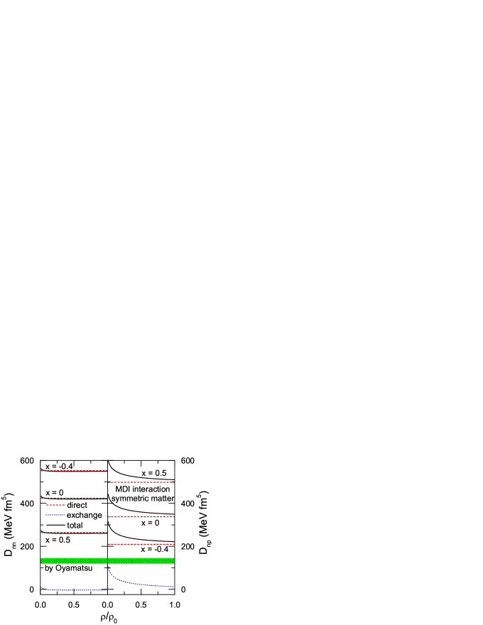
Figure 2: (Color online) Density dependence of effective density-gradient coefficients from different values of $x$ for symmetric nuclear matter. The finite-range direct and exchange contributions are compared, and the value extracted by Oyamatsu Oya03 is also shown.

In Fig. 2, we show the density dependence of effective density-gradient coefficients from different values of $x$ for symmetric nuclear matter. It is seen that the contribution from the finite-range direct interaction is much larger than that from the finite-range exchange interaction. Also, $D_{nn}$ decreases while $D_{np}$ increases with increasing value of $x$. Furthermore, $D_{nn}=D_{pp}$ and $D_{np}=D_{pn}$ for symmetric nuclear matter, whereas all four $D$’s have different values for asymmetric nuclear matter. The density-gradient coefficients extracted from the MDI interaction are, however, much larger than the value of $132\pm 12$ MeV fm⁵ shown in the figure that was used by Oyamatsu Oya03 to fit the nuclear radii and is also consistent with the average value from different Skymre interactions. We note that the large density-gradient coefficients in the presence study is due to our assumption that all of the momentum dependence in the MDI interaction comes from the finite-range exchange term.

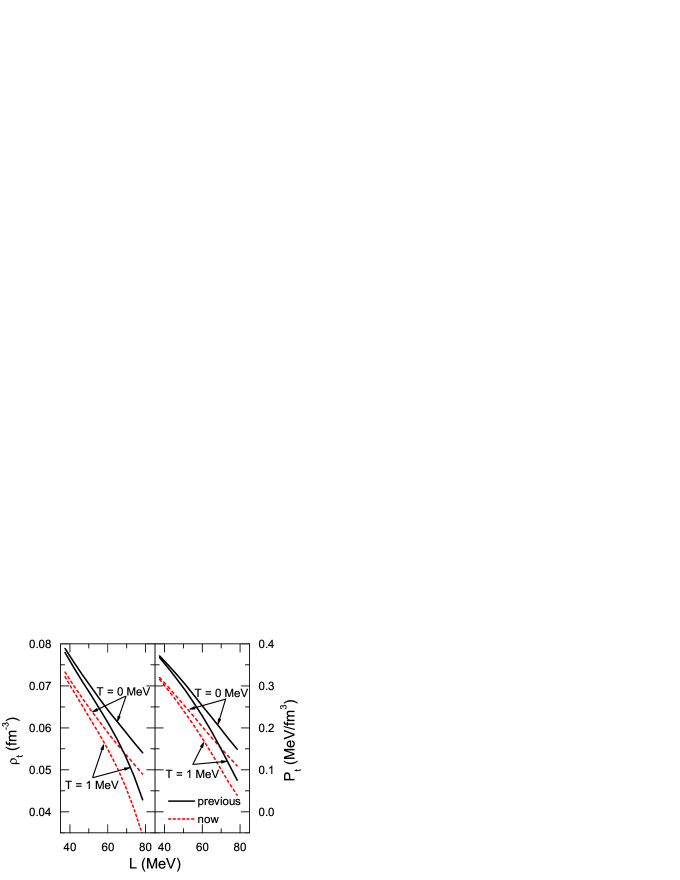
Figure 3: (Color online) The transition density $\rho_{t}$ and pressure $P_{t}$ at the inner edge of neutron star crust as functions of the slope parameter $L$ for $T=0$ MeV and $T=1$ MeV. Previous results XCLM09 ; Xu10 based on density-gradient terms from Ref. Oya03 are also shown for comparison.

In Fig. 3, we compare the transition density and pressure in this study with those from previous calculations XCLM09 ; Xu10 that use the value of $132$ MeV fm⁵ from Ref. Oya03 for the density-gradient coefficients and neglect the exchange Coulomb interaction. It is seen that the present results are smaller than previous ones for neutron star temperatures $T=0$ MeV and $T=1$ MeV. We note that including the exchange Coulomb term for protons slightly increases $\rho_{t}$ while the larger density-gradient coefficients make $\rho_{t}$ smaller. From the latest constraint $L=58\pm 18$ MeV on the density slope of the nuclear symmetry energy, the transition density and pressure are constrained within $0.050$ fm${}^{-3}<\rho_{t}<0.071$ fm^-3 and $0.12$ MeV/fm${}^{3}<P_{t}<0.31$ MeV/fm³ for $T=0$ MeV, and $0.038$ fm${}^{-3}<\rho_{t}<0.070$ fm^-3 and $0.06$ MeV/fm${}^{3}<P_{t}<0.30$ MeV/fm³ for $T=1$ MeV in the present study. Although the transition density is smaller at fixed $L$ compared to our previous results XCLM09 , which leads to a smaller crustal fraction of the moment of inertia for neutron stars and an even stricter constraint on the masses and radii of neutron stars, the upper limit values of $\rho_{t}$ and $P_{t}$ are larger because of the smaller values of $L$. The final constraint on the neutron star mass-radius (M-R) relation is expected to be similar to that in the previous work XCLM09 .

V Summary

Assuming that the momentum dependence in the MDI interaction is entirely due to the finite-range exchange term in the nucleon-nucleon interaction, we have identified the NN interaction potential that underlies the MDI interaction, which has been extensively used in studying isospin effects in intermediate-energy heavy-ion collisions as well as the properties of hot nuclear matter and neutron star matter through the resulting potential energy density in infinite nuclear matter. Using the density matrix expansion, we have obtained an effective zero-range Skyrme-like interaction with density-dependent parameters from the finite-range exchange interaction. Compared to the density-gradient coefficients extracted by Oyamatsu Oya03 and the average value from different Skyrme interactions, the values from the MDI interaction are much larger. Since the momentum dependence in the MDI interaction could also come from the intrinsic momentum dependence in the elementary nucleon-nucleon interaction or be induced by the effects of short-range nucleon-nucleon correlations, we have thus overestimated the effect of the finite-range exchange term. As an application, the resulting interaction is used to determine the transition density and pressure at the inner edge of neutron star crusts based on the linearized Vlasov equation for the neutron star matter. Fortunately, the instability of neutron star matter is dominated by the bulk properties of nuclear matter, the large density-gradient coefficients due to the finite-range interaction do not reduce much the transition density and pressure in neutron stars.

Appendix A From the NN interaction to the potential energy density

The two particle state $|ij>$ in Eq. (3) contains the spatial, spin and isospin parts as

$$|ij>=|i_{r}i_{\sigma}i_{\tau}j_{r}j_{\sigma}j_{\tau}>=|i_{r}j_{r}>|i_{\sigma}j_{\sigma}>|i_{\tau}j_{\tau}>.$$ (98)

For the inner product of spatial state, we have

$$\sum_{i,j}<i_{r}j_{r}|i_{r}j_{r}>$$ (99)

$$= \sum_{i,j}\int<i_{r}j_{r}|\vec{r}_{1}\vec{r}_{2}><\vec{r}_{1}\vec{r}_{2}|i_{r}j_{r}>d^{3}r_{1}d^{3}r_{2}$$

$$= \sum_{i,j}\int\phi_{i}^{\star}(\vec{r}_{1})\phi_{j}^{\star}(\vec{r}_{2})\phi_{i}(\vec{r}_{1})\phi_{j}(\vec{r}_{2})d^{3}r_{1}d^{3}r_{2}$$

$$= \int\rho(\vec{r}_{1})\rho(\vec{r}_{2})d^{3}r_{1}d^{3}r_{2}$$

with $\phi_{i}(\vec{r})=<\vec{r}|i_{r}>$ being the space wave function for particle $i$ and the density $\rho(\vec{r})=\sum_{i}\phi_{i}^{\star}(\vec{r})\phi_{i}(\vec{r})$, and

$$\sum_{i,j}<i_{r}j_{r}|j_{r}i_{r}>$$ (100)

$$= \sum_{i,j}\int<i_{r}j_{r}|\vec{r}_{1}\vec{r}_{2}><\vec{r}_{1}\vec{r}_{2}|j_{r}i_{r}>d^{3}r_{1}d^{3}r_{2}$$

$$= \sum_{i,j}\int\phi_{i}^{\star}(\vec{r}_{1})\phi_{j}^{\star}(\vec{r}_{2})\phi_{j}(\vec{r}_{1})\phi_{i}(\vec{r}_{2})d^{3}r_{1}d^{3}r_{2}$$

$$= \int\rho(\vec{r}_{1},\vec{r}_{2})\rho(\vec{r}_{2},\vec{r}_{1})d^{3}r_{1}d^{3}r_{2}$$

with the off-diagonal density $\rho(\vec{r}_{1},\vec{r}_{2})=\sum_{i}\phi_{i}^{\star}(\vec{r}_{1})\phi_{i}(\vec{r}_{2})$, which reduces to the density when $\vec{r}_{1}=\vec{r}_{2}$.

For the zero-range term $v_{0}=\frac{1}{6}t_{3}(1+x_{3}P_{\sigma})\rho^{\alpha}(\frac{\vec{r}_{1}+\vec{r}_{2}}{2})\delta(\vec{r}_{1}-\vec{r}_{2})$ in the MDI interaction, its direct contribution to the energy can be calculated using the fact that $P_{\sigma}=1/2$ when considering the inner product of spin state in spin saturated matter, and the result is

$$E_{0}^{D} = \frac{1}{2}\sum_{i,j}<ij|v_{0}|ij>$$ (101)

$$= \frac{t_{3}}{12}\int d^{3}r_{1}d^{3}r_{2}\rho(\vec{r}_{1})\rho(\vec{r}_{2})\rho^{\alpha}\left(\frac{\vec{r}_{1}+\vec{r}_{2}}{2}\right)\delta(\vec{r}_{1}-\vec{r}_{2})$$

$$\times \left(1+\frac{x_{3}}{2}\right)$$

$$= \int d^{3}rH_{0}^{D}(\vec{r})$$

with

$$H_{0}^{D}=\frac{t_{3}}{12}\left(1+\frac{x_{3}}{2}\right)\rho^{\alpha+2}.$$ (102)

Its exchange contribution

$$E_{0}^{E}=\frac{1}{2}\sum_{i,j}<ij|v_{0}(-P_{r}P_{\sigma}P_{\tau})|ij>$$ (103)

can be evaluated by using $(1+x_{3}P_{\sigma})(-P_{\sigma}P_{\tau})=-P_{\sigma}P_{\tau}-x_{3}P_{\tau}$ and replacing $P_{\tau}$ by $\delta_{i_{\tau},j_{\tau}}$ when considering the inner product of isospin state, and the result is

$$E_{0}^{E} = -\frac{t_{3}}{12}\int d^{3}r_{1}d^{3}r_{2}\rho(\vec{r}_{1},\vec{r}_{2})\rho(\vec{r}_{2},\vec{r}_{1})\rho^{\alpha}\left(\frac{\vec{r}_{1}+\vec{r}_{2}}{2}\right)$$ (104)

$$\times \delta(\vec{r}_{1}-\vec{r}_{2})\left(\frac{1}{2}+x_{3}\right)\frac{1+\delta^{2}}{2}$$

$$= \int d^{3}rH_{0}^{E}(\vec{r})$$

with

$$H_{0}^{E}=-\frac{t_{3}}{12}\left(\frac{1}{2}+x_{3}\right)\rho^{\alpha+2}\frac{1+\delta^{2}}{2},$$ (105)

and $\delta$ is the isospin asymmetry. The total contribution of the zero-range interaction to the potential energy density is thus

$$H_{0}=H_{0}^{D}+H_{0}^{E}=\frac{t_{3}}{16}\rho^{\alpha+2}\left(1-\frac{1+2x_{3}}{3}\delta^{2}\right).$$ (106)

Comparing it with Eq. (LABEL:MDIV) leads to Eqs. (5)$-$(7).

For the contribution from the finite-range interaction in Eq. (LABEL:MDIv) to the energy, we use in the exchange term the relation $(W+BP_{\sigma}-HP_{\tau}-MP_{\sigma}P_{\tau})(-P_{\sigma}P_{\tau})=M+HP_{\sigma}-BP_{\tau}-WP_{\sigma}P_{\tau}$ to obtain the following total contribution to the potential energy

$$E_{r} = \frac{1}{2}\int d^{3}r_{1}d^{3}r_{2}\{[\rho_{n}(\vec{r}_{1})\rho_{n}(\vec{r}_{2})+\rho_{p}(\vec{r}_{1})\rho_{p}(\vec{r}_{2})]$$ (107)

$$\times \left(W+\frac{B}{2}-H-\frac{M}{2}\right)+2\rho_{n}(\vec{r}_{1})\rho_{p}(\vec{r}_{2})\left(W+\frac{B}{2}\right)$$

$$+ [\rho_{n}(\vec{r}_{1},\vec{r}_{2})\rho_{n}(\vec{r}_{2},\vec{r}_{1})+\rho_{p}(\vec{r}_{1},\vec{r}_{2})\rho_{p}(\vec{r}_{2},\vec{r}_{1})]$$

$$\times \left(M+\frac{H}{2}-B-\frac{W}{2}\right)$$

$$+ 2\left.\rho_{n}(\vec{r}_{1},\vec{r}_{2})\rho_{p}(\vec{r}_{2},\vec{r}_{1})\left(M+\frac{H}{2}\right)\right\}\frac{e^{-\mu|\vec{r}_{1}-\vec{r}_{2}}|}{|\vec{r}_{1}-\vec{r}_{2}|},$$

with the first and second terms being the direct contribution, and the third and fourth terms being the exchange contribution.

To obtain the energy density functional from the finite-range interaction, we introduce the coordinate transformation

$$\vec{r}=(\vec{r}_{1}+\vec{r}_{2})/2,\quad\vec{s}=\vec{r}_{1}-\vec{r}_{2}.$$ (108)

For the direct contribution, we use the approximation of infinite nuclear matter with constant density and make use of the integral $\int d^{3}se^{-\mu s}/s=4\pi/\mu^{2}$ to obtain

$$E_{r}^{D}=\int d^{3}rH_{r}^{D}(\vec{r})$$ (109)

with

$$H_{r}^{D}=\frac{2\pi}{\mu^{2}}\left(W+\frac{B}{2}-\frac{H}{2}-\frac{M}{4}\right)\rho^{2}-\frac{2\pi}{\mu^{2}}\left(\frac{H}{2}+\frac{M}{4}\right)\rho^{2}\delta^{2}.$$ (110)

For the exchange contribution, we express the density matrix in terms of the Fourier transform of the Wigner function, that is

$$\rho_{\tau}\left(\vec{r}+\frac{\vec{s}}{2},\vec{r}-\frac{\vec{s}}{2}\right)=\int d^{3}pf_{\tau}(\vec{r},\vec{p})e^{-i\vec{p}\cdot\vec{s}}.$$ (111)

Substituting Eq. (111) into Eq. (107) and evaluating the Fourier transform of the Yukawa interaction according to

$$\int d^{3}se^{-i(\vec{p}-\vec{p}^{\prime})\cdot\vec{s}}\frac{e^{-\mu s}}{s}=\frac{4\pi}{\mu^{2}}\frac{1}{1+(\vec{p}-\vec{p}^{\prime})^{2}/\mu^{2}},$$ (112)

the exchange contribution of the finite-range interaction to the potential energy is then

$$E_{r}^{E}=\int d^{3}rH_{r}^{E}(\vec{r}),$$ (113)

with

$$H_{r}^{E}(\vec{r}) = \frac{2\pi}{\mu^{2}}\int\frac{d^{3}pd^{3}p^{\prime}}{1+(\vec{p}-\vec{p}^{\prime})^{2}/\mu^{2}}\left[\left(M+\frac{H}{2}-B-\frac{W}{2}\right)\right.$$ (114)

$$\times (f_{n}(\vec{r},\vec{p})f_{n}(\vec{r},\vec{p}^{\prime})+f_{p}(\vec{r},\vec{p})f_{p}(\vec{r},\vec{p}^{\prime}))$$

$$+ \left.\left(M+\frac{H}{2}\right)2f_{n}(\vec{r},\vec{p})f_{p}(\vec{r},\vec{p}^{\prime})\right].$$

Comparing Eqs. (110) and (114) with Eq. (LABEL:MDIV) then allows one to obtain Eqs. (8)$-$(12) for the parameters in the finite-range Yukawa potential in the MDI interaction.

Appendix B Density matrix expansion of the finite-range exchange interaction

Here we follow exactly the same procedure for the density matrix expansion introduced in Ref. Neg72 . To obtain the energy density functional in Eq. (14) from the exchange contribution in Eq. (107), we first use the coordinate transformation given by Eq. (108) to express the density matrix as

$$\rho_{\tau}(\vec{r}_{1},\vec{r}_{2})$$ (115)

$$= \rho_{\tau}(\vec{r}+\frac{\vec{s}}{2},\vec{r}-\frac{\vec{s}}{2})$$

$$= \sum_{i}\phi_{\tau i}^{\star}(\vec{r}+\frac{\vec{s}}{2})\phi_{\tau i}(\vec{r}-\frac{\vec{s}}{2})$$

$$= e^{\frac{\vec{s}}{2}\cdot(\nabla_{1}-\nabla_{2})}\sum_{i}\phi_{\tau i}^{\star}(\vec{r})\phi_{\tau i}(\vec{r}),$$

with $\nabla_{1(2)}$ acting on the first (second) term on the right, and $\phi_{\tau i}$ is the spatial wave function of particle $i$ with isospin $\tau$. The angular average over the direction of $\vec{s}$ is then

$$\frac{1}{4\pi}\int d\Omega_{s}\rho_{\tau}(\vec{r}+\vec{\frac{s}{2}},\vec{r}-\vec{\frac{s}{2}})$$ (116)

$$= \frac{\sinh[\frac{\vec{s}}{2}\cdot(\nabla_{1}-\nabla_{2})]}{\frac{\vec{s}}{2}\cdot(\nabla_{1}-\nabla_{2})}\sum_{i}\phi_{\tau i}^{\star}(\vec{r})\phi_{\tau i}(\vec{r}).$$

Using the Bessel-function expansion

$$\frac{\sinh(xy)}{xy}=\frac{1}{x}\sum_{n=0}^{+\infty}(4n+3)j_{2n+1}(x)Q_{n}(y^{2})$$ (117)

with $j_{2n+1}$ the $(2n+1)$th-order spherical Bessel function and

$$Q_{n}(y^{2})=\frac{1}{2^{2n+1}}\sum_{l=0}^{n}\frac{(4n+2-2l)!y^{2(n-l)}}{l!(2n+1-l)!(2n+1-2l)!},$$ (118)

one obtains by identifying $x\sim k_{\tau}s$ and $y\sim(\nabla_{1}-\nabla_{2})/2k_{\tau}$ with $k_{\tau}$ being the Fermi momentum and keeping up to the third-order Bessel function the following result:

$$\frac{1}{4\pi}\int d\Omega_{s}\rho_{\tau}(\vec{r}+\vec{\frac{s}{2}},\vec{r}-\vec{\frac{s}{2}})$$ (119)

$$= \rho_{SL}(k_{\tau}s)\rho_{\tau}(\vec{r})+g(k_{\tau}s)s^{2}$$

$$\times \left[\frac{1}{4}\nabla^{2}\rho_{\tau}(\vec{r})-\tau_{\tau}(\vec{r})+\frac{3}{5}k_{\tau}^{2}\rho_{\tau}(\vec{r})\right]$$

with $\rho_{SL}(k_{\tau}s)=\frac{3}{k_{\tau}s}j_{1}(k_{\tau}s)$, $g(k_{\tau}s)=\frac{35}{2(k_{\tau}s)^{3}}j_{3}(k_{\tau}s)$ and $\tau_{\tau}(\vec{r})=\sum_{i}|\nabla\phi_{\tau i}(\vec{r})|^{2}$ being the kinetic energy density. By making the approximation

$$\frac{1}{4\pi}\int d\Omega_{s}\rho_{\tau}(\vec{r}+\vec{\frac{s}{2}},\vec{r}-\vec{\frac{s}{2}})\rho_{\tau^{\prime}}(\vec{r}-\vec{\frac{s}{2}},\vec{r}+\vec{\frac{s}{2}})$$ (120)

$$\approx \rho_{\tau}(\vec{r})\rho_{SL}(k_{\tau}s)\rho_{\tau^{\prime}}(\vec{r})\rho_{SL}(k_{\tau^{\prime}}s)$$

$$+ \rho_{\tau}(\vec{r})\rho_{SL}(k_{\tau}s)g(k_{\tau^{\prime}}s)s^{2}$$

$$\times \left[\frac{1}{4}\nabla^{2}\rho_{\tau^{\prime}}(\vec{r})-\tau_{\tau^{\prime}}(\vec{r})+\frac{3}{5}k_{\tau^{\prime}}^{2}\rho_{\tau^{\prime}}(\vec{r})\right]$$

$$+ \rho_{\tau^{\prime}}(\vec{r})\rho_{SL}(k_{\tau^{\prime}}s)g(k_{\tau}s)s^{2}$$

$$\times \left[\frac{1}{4}\nabla^{2}\rho_{\tau}(\vec{r})-\tau_{\tau}(\vec{r})+\frac{3}{5}k_{\tau}^{2}\rho_{\tau}(\vec{r})\right],$$

and using the relation

$$F(\rho_{n},\rho_{p})\nabla^{2}\rho_{n} = -\frac{\partial F(\rho_{n},\rho_{p})}{\rho_{n}}(\nabla\rho_{n})^{2}$$ (121)

$$- \frac{\partial F(\rho_{n},\rho_{p})}{\rho_{p}}\nabla\rho_{n}\cdot\nabla\rho_{p}.$$

we obtain

$$E_{r}^{E}=\int d^{3}rH_{SL}^{E}(\vec{r}),$$ (122)

where $H_{SL}^{E}(\vec{r})$ is the Skymre-like zero-range energy density from the finite-range exchange interaction defined in Eq. (14).

- (1) C.B. Das, S. Das Gupta, C. Gale, and B.A. Li, Phys. Rev. C 67, 034611 (2003).
- (2) L.W. Chen, C.M. Ko, and B.A. Li, Front. Phys. China 2, 327 (2007).
- (3) B.A. Li, L.W. Chen and C.M. Ko, Phys. Rep. 464, 113 (2008).
- (4) M.B. Tsang et al., Phys. Rev. Lett. 92, 062701 (2004).
- (5) L.W. Chen, C.M. Ko, B.A. Li, Phys. Rev. Lett. 94, 032701 (2005).
- (6) B.A. Li and L.W. Chen, Phys. Rev. C 72, 064611 (2005).
- (7) L.W. Chen, C.M. Ko, and B.A. Li, Phys. Rev. C 72, 064309 (2005).
- (8) J. Xu, L.W. Chen, B.A. Li and H.R. Ma, Phys. Rev. C 77, 014302 (2008); Phys. Lett. B650, 347 (2007).
- (9) B.A. Li, L.W. Chen C.M. Ko, P.G. Krastev, A.W. Steiner, and G.C. Yang, J. Phys. G 35, 014044 (2008).
- (10) B.A. Li and A. Steiner, Phys. Lett. B642, 436 (2006).
- (11) P.G. Krastev, B.A. Li and A. Worley, Astrophys. J. 676, 1170 (2008).
- (12) P.G. Krastev, B.A. Li and A. Worley, Phys. Lett. B668, 1 (2008).
- (13) D.H. Wen, B.A. Li, and P.G. Krastev, Phys. Rev. C 80, 025801 (2009).
- (14) W.G. Newton and B.A. Li, Phys. Rev. C 80, 065809 (2009).
- (15) J. Xu, L.W. Chen, B.A. Li, and H.R. Ma, Phys. Rev. C 79, 035802 (2009); Astrophys. J. 697, 1549 (2009).
- (16) C. Gale, G.M. Welke, M. Prakash, S.J. Lee and S. Das Gupta, Phys. Rev. C 41, 1545 (1990).
- (17) J. Decharg and D. Gogny, Phys. Rev. C 21, 1568 (1980).
- (18) D. Vautherin and D.M. Brink, Phys. Rev. C 5, 626 (1972).
- (19) J.W. Negele and D. Vautherin, Phys. Rev. C 5, 1472 (1972); Phys. Rev. C 11, 1031 (1975).
- (20) D.W.L. Sprung, M. Vallieres, X. Campi, and C.M. Ko, Nucl. Phys. A253, 1 (1975).
- (21) J. Xu, L.W. Chen, C.M. Ko and B.A. Li, Phys. Rev. C 81, 055805 (2010).
- (22) M.B. Tsang et al., Phys. Rev. Lett. 102, 122701 (2009).
- (23) L.W. Chen, C.M. Ko, B.A. Li, and J. Xu, arXiv:1004.4672 [nucl-th]
- (24) D.V. Shetty and S.J. Yennello, Pramana-J. Phys. 75, 259 (2010).
- (25) P.K. Panda, D.P. Menezes, C. Providência and J. da Providência, Phys. Rev. C 71, 015801 (2005); P.K. Panda, J. da Providência and C. Providência, Phys. Rev. C 73, 035805 (2006).
- (26) C. Xu and B. A. Li, Phys. Rev. C 81, 044603 (2010).
- (27) E. Chabanat et al., Nucl. Phys. A627, 710 (1997).
- (28) M. Brack, C. Guet and H.B. Håkansson, Phys. Rep. 123, 275 (1985).
- (29) B.K. Jennings, Ph.D. Thesis, McMaster University, Hamilton, Ontario (1976).
- (30) P. Chomaz, M. Colonna and J. Randrup, Phys. Rep. 389, 263 (2004).
- (31) G. Baym, H.A. Bethe and C.J. Pethick, Nucl. Phys. A175, 225 (1971).
- (32) C.J. Pethick, D.G. Ravenhall and C.P. Lorenz, Nucl. Phys. A584, 675 (1995).
- (33) K. Oyamatsu and K. Iida, Phys. Rev. C 75, 015801 (2007).
- (34) K. Oyamatsu and K. Iida, Prog. Theor. Phys. 109, 631 (2003).