Global testing under sparse alternatives: ANOVA, multiple comparisons and the higher criticism

Abstract

Testing for the significance of a subset of regression coefficients in a linear model, a staple of statistical analysis, goes back at least to the work of Fisher who introduced the analysis of variance (ANOVA). We study this problem under the assumption that the coefficient vector is sparse, a common situation in modern high-dimensional settings. Suppose we have $p$ covariates and that under the alternative, the response only depends upon the order of $p^{1-\alpha}$ of those, $0\leq\alpha\leq 1$. Under moderate sparsity levels, that is, $0\leq\alpha\leq 1/2$, we show that ANOVA is essentially optimal under some conditions on the design. This is no longer the case under strong sparsity constraints, that is, $\alpha>1/2$. In such settings, a multiple comparison procedure is often preferred and we establish its optimality when $\alpha\geq 3/4$. However, these two very popular methods are suboptimal, and sometimes powerless, under moderately strong sparsity where $1/2<\alpha<3/4$. We suggest a method based on the higher criticism that is powerful in the whole range $\alpha>1/2$. This optimality property is true for a variety of designs, including the classical (balanced) multi-way designs and more modern “$p>n$” designs arising in genetics and signal processing. In addition to the standard fixed effects model, we establish similar results for a random effects model where the nonzero coefficients of the regression vector are normally distributed.

T1Supported in part by an ONR Grant N00014-09-1-0258.

, and

1 Introduction

1.1 The analysis of variance

Testing whether a subset of covariates have any linear relationship with a quantitative response has been a staple of statistical analysis since Fisher introduced the analysis of variance (ANOVA) in the 1920s MR0346954 . Fisher developed ANOVA in the context of agricultural trials and the test has since then been one of the central tools in the statistical analysis of experiments MR2552961 . As a consequence, there are countless situations in which it is routinely used, in particular, in the analysis of clinical trials MR2154988 or in that of cDNA microarray experiments churchill2002fundamentals , kerr2000analysis , slonim2002patterns , to name just two important areas of biostatistics.

To begin with, consider the simplest design known as the one-way layout,

$$y_{ij}=\mu+\tau_{j}+z_{ij},$$

where $y_{ij}$ is the $i$th observation in group $j$, $\tau_{j}$ is the main effect for the $j$th treatment, and the $z_{ij}$’s are measurement errors assumed to be i.i.d. zero-mean normal variables. The goal is of course to determine whether there is any difference between the treatments. Formally, assuming there are $p$ groups, the testing problem is

$$H_{0}\dvtx\tau_{1}=\tau_{2}=\cdots=\tau_{p}=0,$$

$$H_{1}\dvtx\mbox{at least one }\tau_{j}\neq 0.$$

The classical one-way analysis of variance is based on the well-known $F$-test calculated by all statistical software packages. A characteristic of ANOVA is that it tests for a global null and does not result in the identification of which $\tau_{j}$’s are nonzero.

Taking within-group averages reduces the model to

$$y_{j}=\beta_{j}+z_{j},\qquad j=1,\ldots,p,$$ (1)

where $\beta_{j}=\mu+\tau_{j}$ and the $z_{j}$’s are independent zero-mean Gaussian variables. If we suppose that the grand mean has been removed, so that the overall mean effect vanishes, that is, $\mu=0$, then the testing problem becomes

$$H_{0}\dvtx\beta_{1}=\beta_{2}=\cdots=\beta_{p}=0,$$ (2)

$$H_{1}\dvtx\mbox{at least one }\beta_{j}\neq 0.$$

In order to discuss the power of ANOVA in this setting, assume for simplicity that the variances of the error terms in (1) are known and identical, so that ANOVA reduces to a chi-square test that rejects for large values of $\sum_{j}y_{j}^{2}$. As explained before, this test does not identify which of the $\beta_{j}$’s are nonzero, but it has great power in the sense that it maximizes the minimum power against alternatives of the form $\{{\bolds\beta}\dvtx\sum_{j}\beta_{j}^{2}\geq B\}$ where $B>0$. Such an appealing property may be shown via invariance considerations; see MR941007 and TSH , Chapters 7 and 8.

1.2 Multiple testing and sparse alternatives

A different approach to the same testing problem is to test each individual hypothesis $\beta_{j}=0$ versus $\beta_{j}\neq 0$, and combine these tests by applying a Bonferroni-type correction. One way to implement this idea is by computing the minimum $P$-value and comparing it with a threshold adjusted to achieve a desired significance level. When the variances of the $z_{j}$’s are identical, this is equivalent to rejecting the null when

$$\operatorname{Max}(\mathbf{y})={\max_{j}}|y_{j}|$$ (3)

exceeds a given threshold. From now on, we will refer to this procedure as the Max test. Because ANOVA is such a well established method, it might surprise the reader—but not the specialist—to learn that there are situations where the Max test, though apparently naive, outperforms ANOVA by a wide margin. Suppose indeed that $z_{j}\sim\mathcal{N}(0,1)$ in (1) and consider an alternative of the form $\max_{j}|\beta_{j}|\geq A$ where $A>0$. In this setting, ANOVA requires $A$ to be at least as large as $p^{1/4}$ to provide small error probabilities, whereas the Max test only requires $A$ to be on the order of $(2\log p)^{1/2}$. When $p$ is large, the difference is very substantial. Later in the paper, we shall prove that in an asymptotic sense, the Max test maximizes the minimum power against alternatives of this form. The key difference between these two different classes of alternatives resides in the kind of configurations of parameter values which make the likelihoods under $H_{0}$ and $H_{1}$ very close. For the alternative $\{{\bolds\beta}\dvtx\sum_{j}\beta_{j}^{2}\geq B\}$, the likelihood functions are hard to distinguish when the entries of ${\bolds\beta}$ are of about the same size (in absolute value). For the other, namely, $\{{\bolds\beta}\dvtx\max_{j}|\beta_{j}|\geq A\}$, the likelihood functions are hard to distinguish when there is a single nonzero coefficient equal to $\pm A$.

Multiple hypothesis testing with sparse alternatives is now commonplace, in particular, in computational biology where the data is high-dimensional and we typically expect that only a few of the many measured variables actually contribute to the response—only a few assayed treatments may have a positive effect. For instance, DNA microarrays allow the monitoring of expression levels in cells for thousands of genes simultaneously. An important question is to decide whether some genes are differentially expressed, that is, whether or not there are genes whose expression levels are associated with a response such as the absence/presence of prostate cancer. A typical setup is that the data for the $i$th individual consists of a response or covariate $y_{i}$ (indicating whether this individual has a specific disease or not) and a gene expression profile $y_{ji}$, $1\leq j\leq p$. A standard approach consists in computing, for each gene $j$, a statistic $T_{j}$ for testing the null hypothesis of equal mean expression levels and combining them with some multiple hypothesis procedure Dudoit03 , Efron00 . A possible and simple model in this situation may assume $T_{j}\sim\mathcal{N}(0,1)$ under the null while $T_{j}\sim\mathcal{N}(\beta_{j},1)$ under the alternative. Hence, we are in our sparse detection setup since one typically expects only a few genes to be differentially expressed. Despite the form of the alternative, ANOVA is still a popular method for testing the global null in such problems kerr2000analysis , slonim2002patterns .

1.3 This paper

Our exposition has thus far concerned simple designs, namely, the one-way layout or sparse mean model. This paper, however, is concerned with a much more general problem: we wish to decide whether or not a response depends linearly upon a few covariates. We thus consider the standard linear model

$$\mathbf{y}=\mathbf{X}{\bolds\beta}+\mathbf{z}$$ (4)

with an $n$-dimensional response $\mathbf{y}=(y_{1},\ldots,y_{n})$, a data matrix $\mathbf{X}\in\mathbb{R}^{n\times p}$ (assumed to have full rank) and a noise vector, assumed to be i.i.d. standard normal. The decision problem (2) is whether all the $\beta_{i}$’s are zero or not. We briefly pause to remark that statistical practitioners are familiar with the ANOVA derived $F$-statistic—also known as the model adequacy test—that software packages routinely provide for testing $H_{0}$. Our concern, however, is not at all model adequacy but rather we view the test of the global null as a detection problem. In plain English, we would like to know whether there is signal or whether the data is just noise. A more general problem is to test whether a subset of coordinates of ${\bolds\beta}$ are all zero or not, and, as is well known, ANOVA is in this setup the most popular tool for comparing nested models. We emphasize that our results also apply to such general model comparisons, as we shall see later.

There are many applications of high-dimensional setups in which a response may depend upon only a few covariates. We give a few examples in the life sciences and in engineering; there are, of course, many others:

• Genetics. A single nucleotide polymorphism (SNP) is a form of DNA variation that occurs when at a single position in the genome, multiple (typically two) different nucleotides are found with positive frequency in the population of reference. One then collects information about allele counts at polymorphic locations. Almost all common SNPs have only two alleles so that one records a variable $x_{ij}$ on individual $i$ taking values in $\{0,1,2\}$ depending upon how many copies of, say, the rare allele one individual has at location $j$. One also records a quantitative trait $y_{i}$. Then the problem is to decide whether or not this quantitative trait has a genetic background. In order to scan the entire genome for a signal, one needs to screen between 300,000 and 1,000,000 SNPs. However, if the trait being measured has a genetic background, it will be typically regulated by a small number of genes. In this example, $n$ is typically in the thousands while $p$ is in the hundreds of thousands. The standard approach is to test each hypothesis $H_{j}\dvtx\beta_{j}\neq 0$ by using a statistic depending on the least-squares estimate $\hat{\beta}_{j}$ obtained by fitting the simple linear regression model

  $$y_{i}=\hat{\beta}_{0}+\hat{\beta}_{j}x_{ij}+r_{ij}.$$ (5)

  The global null is then tested by adjusting the significance level to account for the multiple comparisons, effectively implementing a Max test; see Chiararef1 , mccarthy2008genome , for example.

• Communications. A multi-user detection problem typically assumes a linear model of the form (4), where the $j$th column of $\mathbf{X}$, denoted $\mathbf{x}_{j}$, is the channel impulse response for user $j$ so that the received signal from the $j$th user is $\beta_{j}\mathbf{x}_{j}$ (we have $\beta_{j}=0$ in case user $j$ is not sending any message). Note that the mixing matrix $\mathbf{X}$ is often modeled as random with i.i.d. entries. In a strong noise environment, we might be interested in knowing whether information is being transmitted (some $\beta_{j}$’s are not zero) or not. In some applications, it is reasonable to assume that only a few users are transmitting information at any given time. Standard methods include the matched filter detector, which corresponds to the Max test applied to $\mathbf{X}^{T}\mathbf{y}$, and linear detectors, which correspond to variations of the ANOVA $F$-test honig2009advances .

• Signal detection. The most basic problem in signal processing concerns the detection of a signal $S(t)$ from the data $y(t)=S(t)+z(t)$ where $z(t)$ is white noise. When the signal is nonparametric, a popular approach consists in modeling $S(t)$ as a (nearly) sparse superposition of waveforms taken from a dictionary $\mathbf{X}$, which leads to our linear model (4) (the columns of $\mathbf{X}$ are elements from this dictionary). For instance, to detect a multi-tone signal, one would employ a dictionary of sinusoids; to detect a superposition of radar pulses, one would employ a time-frequency dictionary Mallat93 , MallatBook ; and to detect oscillatory signals, one would employ a dictionary of chirping signals. In most cases, these dictionaries are massively overcomplete so that we have more candidate waveforms than the number of samples, that is, $p>n$. Sparse signal detection problems abound, for example the detection of cracks in materials Zhang2000961 , of hydrocarbon from seismic data castagna120 and of tumors in medical imaging breast-tumor .

• Compressive sensing. The sparse detection model may also arise in the area of compressive sensing CRT , OptimalRecovery , Donoho-CS , a novel theory which asserts that it is possible to accurately recover a (nearly) sparse signal—and by extension, a signal that happens to be sparse in some fixed basis or dictionary—from the knowledge of only a few of its random projections. In this context, the $n\times p$ matrix $\mathbf{X}$ with $n\ll p$ may be a random projection such as a partial Fourier matrix or a matrix with i.i.d. entries. Before reconstructing the signal, we might be interested in testing whether there is any signal at all in the first place.

All these examples motivate the study of two classes of sparse alternatives: [(1)]

Sparse fixed effects model (SFEM). Under the alternative, the regression vector ${\bolds\beta}$ has at least $S$ nonzero coefficients exceeding $A$ in absolute value.

Sparse random effects model (SREM). Under the alternative, the regression vector ${\bolds\beta}$ has at least $S$ nonzero coefficients assumed to be i.i.d. normal with zero mean and variance $\tau^{2}$. In both models, we set $S=p^{1-\alpha}$, where $\alpha\in(0,1)$ is the sparsity exponent. Our purpose is to study the performance of various test statistics for detecting such alternatives.

1.4 Prior work

To introduce our results and those of others, we need to recall a few familiar concepts from statistical decision theory. From now on, $\Omega$ denotes a set of alternatives, namely, a subset of $\mathbb{R}^{p}\setminus\{0\}$ and $\pi$ is a prior on $\Omega$. The Bayes risk of a test $T=T(\mathbf{X},\mathbf{y})$ for testing ${\bolds\beta}={\mathbf{0}}$ versus ${\bolds\beta}\sim\pi$ when $H_{0}$ and $H_{1}$ occur with the same probability is defined as the sum of its probability of type I error (false alarm) and its average probability of type II error (missed detection). Mathematically,

$$\operatorname{Risk}_{\pi}(T):=\mathbb{P}_{\mathbf{0}}(T=1)+\pi[\mathbb{P}_{\bolds\beta}(T=0)],$$ (6)

where $\mathbb{P}_{\bolds\beta}$ is the probability distribution of $\mathbf{y}$ given by the model (4) and $\pi[\cdot]$ is the expectation with respect to the prior $\pi$. If we consider the linear model in the limit of large dimensions, that is, $p\to\infty$ and $n=n(p)\to\infty$, and a sequence of priors $\{\pi_{p}\}$, then we say that a sequence of tests $\{T_{n,p}\}$ is asymptotically powerful if $\lim_{p\to\infty}\operatorname{Risk}_{\pi_{p}}(T_{n,p})=0$. We say that it is asymptotically powerless if $\liminf_{p\to\infty}\operatorname{Risk}_{\pi_{p}}(T_{n,p})\geq 1$. When no prior is specified, the risk is understood as the worst-case risk defined as

$$\operatorname{Risk}(T):=\mathbb{P}_{\mathbf{0}}(T=1)+\max_{{\bolds\beta}\in\Omega}\mathbb{P}_{\bolds\beta}(T=0).$$

With our modeling assumptions, ANOVA for testing ${\bolds\beta}={\mathbf{0}}$ versus ${\bolds\beta}\neq{\mathbf{0}}$ reduces to the chi-square test that rejects for large values of $\|\mathbf{P}\mathbf{y}\|^{2}$, where $\mathbf{P}$ is the orthogonal projection onto the range of $\mathbf{X}$. Since under the alternative, $\|\mathbf{P}\mathbf{y}\|^{2}$ has the chi-square distribution with $\min(n,p)$ degrees of freedom and noncentrality parameter $\|\mathbf{X}{\bolds\beta}\|^{2}$, a simple argument shows that ANOVA is asymptotically powerless when

$$\|\mathbf{X}{\bolds\beta}\|^{2}/\sqrt{\min(n,p)}\to 0,$$ (7)

and asymptotically powerful if the same quantity tends to infinity. This is congruent with the performance of ANOVA in a standard one-way layout; see MR2062823 , who obtain the weak limit of the ANOVA $F$-ratio under various settings.

Consider the sparse fixed effects alternative now. We prove that ANOVA is still essentially optimal under mild levels of sparsity corresponding to $\alpha\in[0,1/2]$ but not under strong sparsity where $\alpha\in(1/2,1]$. In the sparse mean model (1) where $\mathbf{X}$ is the identity, ANOVA is suboptimal, requiring $A$ to grow as a power of $p$; this is simply because (7) becomes $A^{2}S/\sqrt{p}\to 0$ when all the nonzero coefficients are equal to $A$ in absolute value. In contrast, the Max test is asymptotically powerful when $A$ is on the order of $\sqrt{\log p}$ but is only optimal under very strong sparsity, namely, for $\alpha\in[3/4,1]$. It is possible to improve on the Max test in the range $\alpha\in(1/2,3/4)$ and we now review the literature which only concerns the sparse mean model, $\mathbf{X}=\mathbf{I}_{p}$. Set

$$\rho^{*}(\alpha)=\cases{\alpha-1/2,&\quad$1/2<\alpha<3/4$,\vspace*{2pt}\cr\bigl{(}1-\sqrt{1-\alpha}\bigr{)}^{2},&\quad$3/4\leq\alpha<1$.}$$ (8)

Then Ingster Ingster99 showed that if $A=\sqrt{2r\log p}$ with $r<\rho^{*}(\alpha)$ fixed as $p\to\infty$, then all sequences of tests are asymptotically powerless. In the other direction, he showed that there is an asymptotically powerful sequence of tests if $r>\rho^{*}(\alpha)$. See also the work of Jin jinPhD . Donoho and Jin dj04 analyzed a number of testing procedures in this setting, and, in particular, the higher criticism of Tukey which rejects for large values of

$$\mathrm{HC}^{*}(\mathbf{y})=\sup_{t>0}\frac{\#\{i\dvtx|y_{i}|>t\}-2p\bar{\Phi}(t)}{\sqrt{2p\bar{\Phi}(t)(1-2\bar{\Phi}(t))}},$$

where $\bar{\Phi}$ denotes the survival function of a standard normal random variable. They showed that the higher criticism is powerful within the detection region established by Ingster. Hall and Jin hj08 , hj09 have recently explored the case where the noise may be correlated, that is, $\mathbf{z}\sim\mathcal{N}({\mathbf{0}},\mathbf{V})$ and the covariance matrix $\mathbf{V}$ is known and has full rank. Letting $\mathbf{V}=\mathbf{L}\mathbf{L}^{T}$ be a Cholesky factorization of the covariance matrix, one can whiten the noise in $\mathbf{y}={\bolds\beta}+\mathbf{z}$ by multiplying both sides by $\mathbf{L}^{-1}$, which yields $\tilde{\mathbf{y}}=\mathbf{L}^{-1}{\bolds\beta}+\tilde{\mathbf{z}}$; $\tilde{\mathbf{z}}$ is now white noise, and this is a special case of the linear model (4). When the design matrix is triangular with coefficients decaying polynomially fast away from the diagonal, hj09 proves that the detection threshold remains unchanged, and that a form of higher criticism still achieves asymptotic optimality.

There are few other theoretical results in the literature, among which MR2278336 develops a locally most powerful (score) test in a setting similar to SREM; here, “locally” means that this property only holds for values of $\tau$ sufficiently close to zero. The authors do not provide any minimal value of $\tau$ that would guarantee the optimality of their method. However, since their score test resembles the ANOVA $F$-test, we suggest that it is only optimal for very small values of $\tau$ corresponding to mild levels of sparsity, that is, $\alpha<1/2$.

Since the submission of our paper, a manuscript by Ingster, Tsybakov and Verzelen ingster2010detection , also considering the detection of a sparse vector in the linear regression model, has become publicly available. We comment on differences in Section 3.

In the signal processing literature, a number of applied papers consider the problem of detecting a signal expressed as a linear combination in a dictionary castagna120 , Zhang2000961 , MR1956096 . However, the extraction of the salient signal is often the end goal of real signal processing applications so that research has focused on estimation rather than pure detection. As a consequence, one finds a literature entirely focused on estimation rather than on testing whether the data is just white noise or not. Examples of pure detection papers include sparse-detection , CS-detection , meng-sparse . In sparse-detection , the authors consider detection by matched filtering, which corresponds to the Max test, and perform simulations to assess its power. The authors in CS-detection assume that ${\bolds\beta}$ is approximately known and examine the performance of the corresponding matched filter. Finally, the paper meng-sparse proposes a Bayesian approach for the detection of sparse signals in a sensor network for which the design matrix is assumed to have some polynomial decay in terms of the distance between sensors.

1.5 Our contributions

We show that if the predictor variables are not too correlated, there is a sharp detection threshold in the sense that no test is essentially better than a coin toss when the signal strength is below this threshold, and that there are statistics which are asymptotically powerful when the signal strength is above this threshold. This threshold is the same as that one gets for the sparse mean problem. Therefore, this work extends the earlier results and methodologies cited above Ingster99 , jinPhD , dj04 , hj08 , hj09 , and is applicable to the modern high-dimensional situation where the number of predictors may greatly exceed the number of observations.

A simple condition under which our results hold is a low-coherence assumption. Let $\mathbf{x}_{1},\ldots,\mathbf{x}_{p}$ be the column vectors of $\mathbf{X}$, assumed to be normalized; this assumption is merely for convenience since it simplifies the exposition, and is not essential. Then if a large majority of all pairs of predictors have correlation less than $\gamma$ with $\gamma=O(p^{-1/2+\varepsilon})$ for each $\varepsilon>0$ (the real condition is weaker), then the results for the sparse mean model (1) apply almost unchanged. Interestingly, this is true even when the ratio between the number of observations and the number of variables is negligible, that is, $n/p\to 0$. In particular, $A=\sqrt{2\rho^{*}(\alpha)\log p}$ is the sharp detection threshold for SFEM (sparse fixed effects model). Moreover, applying the higher criticism, not to the values of $\mathbf{y}$, but to those of $\mathbf{X}^{T}\mathbf{y}$ is asymptotically powerful as soon as the nonzero entries of ${\bolds\beta}$ are above this threshold; this is true for all $\alpha\in(1/2,1]$. In contrast, the Max test applied to $\mathbf{X}^{T}\mathbf{y}$ is only optimal in the region $\alpha\in[3/4,1]$. We derive the sharp threshold for SREM as well, which is at $\tau=\sqrt{\alpha/(1-\alpha)}$. We show that the Max tests and the higher criticism are essentially optimal in this setting as well for all $\alpha\in(1/2,1]$, that is, they are both asymptotically powerful as soon as the signal-to-noise ratio permits.

Before continuing, it may be a good idea to give a few examples of designs obeying the low-coherence assumption (weak correlations between most of the predictor variables) since it plays an important role in our analysis:

• Orthogonal designs. This is the situation where the columns of $\mathbf{X}$ are orthogonal so that $\mathbf{X}^{T}\mathbf{X}$ is the $p\times p$ identity matrix (necessarily, $p\leq n$). Here the coherence is of course the lowest since $\gamma(\mathbf{X})=0$.

• Balanced, one-way designs. As in a clinical trial comparing $p$ treatments, assume a balanced, one-way design with $k$ replicates per treatment group and with the grand mean already removed. This corresponds to the linear model (4) with $n=pk$ and, since we assume the predictors to have norm $1$,

  $$\mathbf{X}=\frac{1}{\sqrt{k}}\left[\matrix{{\mathbf{1}}&{\mathbf{0}}&\cdots&{\mathbf{0}}\cr{\mathbf{0}}&{\mathbf{1}}&\cdots&{\mathbf{0}}\cr\vdots&\vdots&\vdots&\vdots\cr{\mathbf{0}}&{\mathbf{0}}&\cdots&{\mathbf{1}}}\right]\in\mathbb{R}^{n\times p},$$ (9)

  where each vector in this block representation is $k$-dimensional. This is in fact an example of orthogonal design. Note that our results apply even under the standard constraint ${\mathbf{1}}^{T}{\bolds\beta}=0$.

• Concatenation of orthonormal bases. Suppose that $p=nk$ and that $\mathbf{X}$ is the concatenation of $k$ orthonormal bases in $\mathbb{R}^{n}$ jointly used as to provide an efficient signal representation. Then our result applies provided that $k=O(n^{\varepsilon}),\forall\varepsilon>0$ and that our bases are mutually incoherent so that $\gamma$ is sufficiently small (for examples of incoherent bases see, e.g., MR1872845 ).

• Random designs. As in some compressive sensing and communications applications, assume that $\mathbf{X}$ has i.i.d. normal entries with columns subsequently normalized (the column vectors are sampled independently and uniformly at random on the unit sphere). Such a design is close to orthogonal since $\gamma\leq\sqrt{5(\log p)/n}$ with high probability. This fact follows from a well-known concentration inequality for the uniform distribution on the sphere MR1849347 . The exact same bound applies if the entries of $\mathbf{X}$ are instead i.i.d. Rademacher random variables.

We return to the discussion of our statistics and note that the higher criticism and the Max test applied to $\mathbf{X}^{T}\mathbf{y}$ are exceedingly simple methods with a straightforward implementation running in $O(np)$ flops. This brings us to two important points: [(1)]

In the classical sparse mean model, Bonferroni-type multiple testing (the Max test) is not optimal when the sparsity level is moderately strong, that is, when $1/2<\alpha<3/4$ dj04 . This has direct implications in the fields of genetics and genomics where this is the prevalent method. The same is true in our more general model and it implies, for example, that the matched filter detector in wireless multi-user detection is suboptimal in the same sparsity regime.

We elaborate on this point because this carries an important message. When the sparsity level is moderately strong, the higher criticism method we propose is powerful in situations where the signal amplitude is so weak that the Max test is powerless. This says that one can detect a linear relationship between a response $\mathbf{y}$ and a few covariates even though those covariates that are most correlated with $\mathbf{y}$ are not even in the model. Put differently, if we assign a $P$-value to each hypothesis $\beta_{j}=0$ (computed from a simple linear regression as discussed earlier), then the case against the null is not in the tail of these $P$-values but in the bulk, that is, the smallest $P$-values may not carry any information about the presence of a signal. In the situation we describe, the smallest $P$-values most often correspond to true null hypotheses, sometimes in such a way that the false discovery rate (FDR) cannot be controlled at any level below 1; and yet, the higher criticism has full power.

Though we developed the idea independently, the higher criticism applied to $\mathbf{X}^{T}\mathbf{y}$ is similar to the innovated higher criticism of Hall and Jin hj09 , which is specifically designed for time series. Not surprisingly, our results and arguments bear some resemblance with those of Hall and Jin hj09 . We have already explained how their results apply when the design matrix is triangular (and, in particular, square) and has sufficiently rapidly decaying coefficients away from the diagonal. Our results go much further in the sense that (1) they include designs that are far from being triangular or even square, and (2) they include designs with coefficients that do not necessarily follow any ordered decay pattern. On the technical side, Hall and Jin astutely reduce matters to the case where the design matrix is banded, which greatly simplifies the analysis. In the general linear model, it is not clear how a similar reduction would operate especially when $n<p$—at the very least, we do not see a way—and one must deal with more intricate dependencies in the noise term $\mathbf{X}^{T}\mathbf{z}$.

As we have remarked earlier, we have discussed testing the global null ${\bolds\beta}={\mathbf{0}}$, whereas some settings obviously involve nuisance parameters as in the comparison of nested models. Examples of nuisance parameters include the grand mean in a balanced, one-way design or, more generally, the main effects or lower-order interactions in a multi-way layout. In signal processing, the nuisance term may represent clutter as opposed to noise. In general, we have

$$\mathbf{y}=\mathbf{X}^{(0)}{\bolds\beta}^{(0)}+\mathbf{X}^{(1)}{\bolds\beta}^{(1)}+\mathbf{z},$$

where ${\bolds\beta}^{(0)}$ is the vector of nuisance parameters, and ${\bolds\beta}^{(1)}$ the vector we wish to test. Our results concerning the performance of ANOVA, the higher criticism or the Max test apply provided that the column spaces of $\mathbf{X}^{(0)}$ and $\mathbf{X}^{(1)}$ be sufficiently far apart. This occurs in lots of applications of interest. In the case of the balanced, multi-way design, these spaces are actually orthogonal. In signal processing, these spaces will also be orthogonal if the column space of $\mathbf{X}^{(0)}$ spans the low-frequencies while we wish to detect the presence of a high-frequency signal. The general mechanism which allows us to automatically apply our results is to simply assume that $\mathbf{P}_{0}\mathbf{X}^{(1)}$, where $\mathbf{P}_{0}$ is the orthogonal projector with the range of $\mathbf{X}^{(0)}$ as null space, obeys the conditions we have for $\mathbf{X}$.

1.6 Organization of the paper

The paper is organized as follows. In Section 2 we consider orthogonal designs and state results for the classical setting where no sparsity assumption is made on the regression vector ${\bolds\beta}$, and the setting where ${\bolds\beta}$ is mildly sparse. In Section 3 we study designs in which most pairs of predictor variables are only weakly correlated; this part contains our main results. In Section 4 we focus on some examples of designs with full correlation structure, in particular, multi-way layouts with embedded constraints. Section 5 complements our study with some numerical experiments, and we close the paper with a short discussion, namely, Section 6. Finally, the proofs are gathered in a supplementary file unstructured-suppl .

1.7 Notation

We provide a brief summary of the notation used in the paper. Set $[p]=\{1,\ldots,p\}$ and for a subset $\mathcal{J}\subset[p]$, let $|\mathcal{J}|$ be its cardinality. Bold upper (resp., lower) case letters denote matrices (resp., vectors), and the same letter not bold represents its coefficients, for example, $a_{j}$ denotes the $j$th entry of $\mathbf{a}$. For an $n\times p$ matrix $\mathbf{A}$ with column vectors $\mathbf{a}_{1},\ldots,\mathbf{a}_{p}$, and a subset $\mathcal{J}\subset[p]$, $\mathbf{A}_{\mathcal{J}}$ denotes the $n$-by-$|\mathcal{J}|$ matrix with column vectors $\mathbf{a}_{j},j\in\mathcal{J}$. Likewise, $\mathbf{a}_{\mathcal{J}}$ denotes the vector $(a_{j},j\in\mathcal{J})$. The Euclidean norm of a vector is $\|\mathbf{a}\|$ and the sup-norm $\|\mathbf{a}\|_{\infty}$. For a matrix $\mathbf{A}=(a_{ij})$, $\|\mathbf{A}\|_{\infty}=\sup_{i,j}|a_{ij}|$, and this needs to be distinguished from $\|\mathbf{A}\|_{\infty,\infty}$, which is the operator norm induced by the sup norm, $\|\mathbf{A}\|_{\infty,\infty}=\sup_{\|\mathbf{x}\|_{\infty}\leq 1}\|\mathbf{A}\mathbf{x}\|_{\infty}$. The Frobenius (Euclidean) norm of $\mathbf{A}$ is $\|\mathbf{A}\|_{F}$. $\Phi$ (resp., $\phi$) denotes the cumulative distribution (resp., density) function of a standard normal random variable, and $\bar{\Phi}$ its survival function. For brevity, we say that ${\bolds\beta}$ is $S$-sparse if ${\bolds\beta}$ has exactly $S$ nonzero coefficients. Finally, we say that a random variable $X\sim F_{X}$ is stochastically smaller than $Y\sim F_{Y}$, denoted $X\leq^{\mathrm{sto}}Y$, if $F_{X}(t)\geq F_{Y}(t)$ for all scalar $t$.

2 Orthogonal designs

This section introduces some results for the orthogonal design in which the columns of $\mathbf{X}$ are orthonormal, that is, $\mathbf{X}^{T}\mathbf{X}=\mathbf{I}_{p}$. While from the analysis viewpoint there is little difference with the case where $\mathbf{X}$ is the identity matrix, this is of course a special case of our general results, and this section may also serve as a little warm-up. Our first result, which is a special case of Proposition 2, determines the range of sparse alternatives for which ANOVA is essentially optimal.

Proposition 1

Suppose $\mathbf{X}$ is orthogonal and let the number of nonzero coefficients be $S=p^{1-\alpha}$ with $\alpha\in[0,1/2]$. In SFEM (resp., SREM), all sequences of tests are asymptotically powerless if $A^{2}S/p^{1/2}\to 0$ (resp.,$\tau^{2}S/p^{1/2}\to 0$).

Returning to our earlier discussion, it follows from (7) and the lower bound $\|\mathbf{X}\beta\|^{2}=\|\beta\|^{2}\geq A^{2}S$ that ANOVA has full asymptotic power whenever $A^{2}S/p^{1/2}\to\infty$. Therefore, comparing this with the content of Proposition 1 reveals that ANOVA is essentially optimal in the moderately sparse range corresponding to $\alpha\in[0,1/2]$.

The second result of this section is that under an $n\times p$ orthogonal design, the detection threshold is the same as if $\mathbf{X}$ were the identity. We need a little bit of notation to develop our results. As in dj04 , define

$$\rho_{\mathrm{Max}}(\alpha)=\bigl{(}1-\sqrt{1-\alpha}\bigr{)}^{2},$$

and observe that with $\rho^{*}(\alpha)$ as in (8),

$$\cases{\rho^{*}(\alpha)<\rho_{\mathrm{Max}}(\alpha),&\quad$1/2\leq\alpha<3/4$,\cr\rho^{*}(\alpha)=\rho_{\mathrm{Max}}(\alpha),&\quad$3/4\leq\alpha\leq 1$.}$$

We will also set a detection threshold for SREM defined by

$$\rho^{*}_{\mathrm{rand}}(\alpha)=\sqrt{\alpha/(1-\alpha)}.$$ (10)

With these definitions, the following theorem compares the performance of the higher criticism and the Max test.

Theorem 1

Suppose $\mathbf{X}$ is orthogonal and assume the sparsity exponent obeys $\alpha\in(1/2,1]$. [(1)]

In SFEM, all sequences of tests are asymptotically powerless if $A=\sqrt{2r\log p}$ with $r<\rho^{*}(\alpha)$. Conversely, the higher criticism applied to $|\mathbf{x}_{1}^{T}\mathbf{y}|,\ldots,\break|\mathbf{x}_{p}^{T}\mathbf{y}|$ is asymptotically powerful if $r>\rho^{*}(\alpha)$. Also, the Max test is asymptotically powerful if $r>\rho_{\mathrm{Max}}(\alpha)$ and powerless if $r<\rho_{\mathrm{Max}}(\alpha)$.

In SREM, all sequences of tests are asymptotically powerless if $\tau<\rho^{*}_{\mathrm{rand}}(\alpha)$. Conversely, both the higher criticism and the Max test applied to $|\mathbf{x}_{1}^{T}\mathbf{y}|,\ldots,|\mathbf{x}_{p}^{T}\mathbf{y}|$ are asymptotically powerful if $\tau>\rho^{*}_{\mathrm{rand}}(\alpha)$. In the upper bounds, $r$ and $\tau$ are fixed while $p\to\infty$.

To be absolutely clear, the statements for SFEM may be understood either in the worst-case risk sense or under the uniform prior on the set of $S$-sparse vectors with nonzero coefficients equal to $\pm A$. For SREM, the prior simply selects the support of ${\bolds\beta}$ uniformly at random. After multiplying the observation by $\mathbf{X}^{T}$, matters are reduced to the case of the identity design for which the performance of the higher criticism and the Max test have been established in SFEM dj04 . The result for the sparse random model is new and appears in more generality in Theorem 5.

To conclude, the situation concerning orthogonal designs is very clear. In SFEM, for instance, if the sparsity level is such that $\alpha\leq 1/2$, then ANOVA is asymptotically optimal whereas the higher criticism is optimal if $\alpha>1/2$. In contrast, the Max test is only optimal in the range $\alpha\geq 3/4$.

3 Weakly correlated designs

We begin by introducing a model of design matrices in which most of the variables are only weakly correlated. Our model depends upon two parameters, and we say that a $p\times p$ correlation matrix $\mathbf{C}$ belongs to the class $\mathcal{S}_{p}(\gamma,\Delta)$ if and only if it obeys the following two properties:

• Strong correlation property. This requires that for all $j\neq k$,

  $$|c_{jk}|\leq 1-(\log p)^{-1}.$$

  That is, all the correlations are bounded above by $1-(\log p)^{-1}$. In the limit of large $p$, this is not an assumption and we will later explain how one can relax this even further.

• Weak correlation property. This is the main assumption and this requires that for all $j$,

  $$\bigl{|}\{k\dvtx|c_{jk}|>\gamma\}\bigr{|}\leq\Delta.$$

  Note that for $\gamma\leq 1$, $\Delta\geq 1$ since $c_{jj}=1$. Fix a variable $\mathbf{x}_{j}$. Then at most $\Delta-1$ other variables have a correlation exceeding $\gamma$ with $\mathbf{x}_{j}$.

Our only real condition caps the number of variables that can have a correlation with any other above a threshold $\gamma$. An orthogonal design belongs to $\mathcal{S}_{p}(0,1)$ since all the correlations vanish. With high probability, the Gaussian and Rademacher designs described earlier belong to $\mathcal{S}_{p}(\gamma,1)$ with $\gamma=\sqrt{5(\log p)/n}$.

3.1 Lower bound on the detectability threshold

The main result of this paper is that if the predictor variables are not highly correlated, meaning that the quantities $\gamma$ and $\Delta$ above are sufficiently small, then there are computable detection thresholds for our sparse alternatives that are very similar or identical to those available for orthogonal designs.

We begin by studying lower bounds and for SFEM, these may be understood either in a worst-case sense or under the prior where ${\bolds\beta}$ is uniformly distributed among all $S$-sparse vectors with nonzero coefficients equal to $\pm A$. For SREM, these hold under a prior generating the support uniformly at random. We first consider mildly sparse alternatives.

Proposition 2

Suppose that $\mathbf{X}^{T}\mathbf{X}\in\mathcal{S}_{p}(\gamma,1)$ and let $S=p^{1-\alpha}$ with $\alpha\in[0,1/2]$. In SFEM (resp., SREM), all sequences of tests are asymptotically powerless if $A^{2}S(p^{-1/2}+\gamma\log p)\to 0$ [resp., $\tau^{2}S(p^{-1/2}+\gamma)\to 0$].

In order to interpret this proposition, we note that $\gamma$ will usually be at least as large as $n^{-1/2}$, as shown just below.

In Proposition 2 we have required that $\Delta=1$ in order to derive sharp results. Moving now to sparser alternatives, we allow for $\Delta$ to increase with $p$, although very slowly, while the condition on $\gamma$ remains essentially the same.

Theorem 2

Assume the sparsity exponent obeys $\alpha\in(1/2,1]$, and suppose that $\mathbf{X}^{T}\mathbf{X}\in\mathcal{S}_{p}(\gamma,\Delta)$ with the following parameter asymptotics: (1) $\Delta=O(p^{\varepsilon})$, for all $\varepsilon>0$, and (2) $\gamma p^{1-\alpha}(\log p)^{4}\to 0$. In SFEM (resp., SREM), all sequences of tests are asymptotically powerless if $A=\sqrt{2r\log p}$ with $r<\rho^{*}(\alpha)$ [resp., $\tau<\rho^{*}_{\mathrm{rand}}(\alpha)$].

The result is essentially the same in the case of a balanced, multi-way design with the usual linear constraints. We comment on this point at the end of the proof of Theorem 2.

The reader may be surprised to see that the number $n$ of observations does not explicitly appear in the above lower bounds. The sample size appears implicitly, however, since it must be large enough for the class $\mathcal{S}_{p}(\gamma,\Delta)$ to be nonempty. Assume $\Delta=1$, for instance, and that $p\geq n$. Then by the lower bound MR1984549 , equation (12), we have

$$\gamma\geq\sqrt{(p-n)/(np)}.$$ (11)

For instance, $\gamma\geq 1/\sqrt{2n}$ if $p\geq 2n$.

As a technical aside, we remark that the lower bounds hold under the strong correlation assumption

$$|c_{jk}|\leq 1-\delta$$

for any $\delta<1$, provided that $\gamma\delta^{-2}p^{1-\alpha}(\log p)^{3/2}\to 0$. We shall prove this more general statement, and the theorem is thus a special case corresponding to $\delta=(\log p)^{-1}$.

We pause to compare with the results of the recent paper ingster2010detection . The lower bounds in ingster2010detection are the same as ours (for SFEM) except that they impose slightly weaker conditions on $\gamma$. In Proposition 2, their condition is $A^{2}S(p^{-1/2}+\gamma)\to 0$, and in Theorem 2, their condition is $\gamma p^{1-\alpha}\log p\to 0$.

3.2 Upper bound on the detectability threshold

We now turn to upper bounds and, unless stated otherwise, these assume the following models:

• For SFEM, we assume that ${\bolds\beta}$ has a support generated uniformly at random and that its nonzero coefficients have random signs.

• For SREM, we assume that ${\bolds\beta}$ has a support generated uniformly at random.

We require that the support of ${\bolds\beta}$ be generated uniformly at random and, in SFEM, that the signs of its coefficients be also random to rule out situations where cancellations occur, making the signal strength potentially too small (and possibly vanish) to allow for reliable detection.

We begin by studying the performance of ANOVA when the alternative is not that sparse. We state our result for $\Delta=1$ in accordance with the lower bound (Proposition 2), although the result holds when $\Delta$ obeys $\Delta=O(p^{\varepsilon})$ for all $\varepsilon>0$.

Proposition 3

Assume that $\mathbf{X}^{T}\mathbf{X}\in\mathcal{S}_{p}(\gamma,1)$ and let $S=p^{1-\alpha}$.

• Assume $\gamma\log p\to 0$. Then, in SFEM, ANOVA is asymptotically powerful (resp., powerless) when $A^{2}S/\sqrt{\min(n,p)}\rightarrow\infty$ (resp., $\to 0$).

• Assume $\gamma\to 0$. Then, in SREM, ANOVA is asymptotically powerful (resp., powerless) when $\tau^{2}S/\sqrt{\min(n,p)}\rightarrow\infty$ (resp., $\to 0$).

Note that this holds for all values of $\alpha$.

For example, consider an $n\times p$ Gaussian design with $p>n$. For this design $\gamma\asymp\sqrt{(\log p)/n}$ (in probability). Hence, assuming $(\log p)^{3/2}/\sqrt{n}\to 0$, Proposition 3 says that, in SFEM, the ANOVA test is powerful when $A^{2}S/\sqrt{n}\rightarrow\infty$. We contrast this with Proposition 2, which says that, in the same context and assuming that $\alpha\in[0,1/2]$, all methods are powerless when $A^{2}S(\log p)^{3/2}/\sqrt{n}\rightarrow 0$. Hence, in this moderately sparse setting where $\alpha\in[0,1/2]$, if one ignores the $(\log p)^{3/2}$ factor (we do not know whether Proposition 2 is tight), then one can say that ANOVA achieves the optimal detection boundary. However, as we will see in Theorems 3, 4 and 5, ANOVA is far from optimal in the strongly sparse case when $\alpha>1/2$.

Compared with Proposition 2, the condition on $\gamma$ is substantially weaker. More importantly, there appears to be a major discrepancy when $n$ is negligible compared to $p$ because $\sqrt{\min(n,p)}$ replaces $\sqrt{p}$. This is illusory, however, as the lower bound on $\gamma$ displayed in (11) implies that the condition on $A$ in Proposition 2 matches that of Proposition 3 up to a $\log p$ factor.

Turning to sparser alternatives, we apply the higher criticism to $\mathbf{X}^{T}\mathbf{y}$ and for $t>0$, put

$$H(t)=\frac{|\{j\dvtx|\mathbf{x}_{j}^{T}\mathbf{y}|>t\}|-2p\bar{\Phi}(t)}{\sqrt{2p\bar{\Phi}(t)(1-2\bar{\Phi}(t))}}.$$

The innovated higher criticism of Hall and Jin hj09 resembles $\sup_{t>0}H(t):=\mathrm{HC}^{*}(\mathbf{X}^{T}\mathbf{y})$, the main difference being that they apply a threshold to the entries of $\mathbf{X}$ before multiplying by $\mathbf{X}^{T}$. Here, to facilitate the analysis, we search for the maximum on a discrete grid and define

$$H^{*}(s)=\max\bigl{\{}H(t)\dvtx t\in\bigl{[}s,\sqrt{5\log p}\bigr{]}\cap\mathbb{N}\bigr{\}}.$$

Theorem 3

Assume the sparsity exponent obeys $\alpha\in(1/2,1]$ and suppose that $\mathbf{X}^{T}\mathbf{X}\in\mathcal{S}_{p}(\gamma,\Delta)$ with the following parameter asymptotics: (1) $\Delta=O(p^{\varepsilon})$, for all $\varepsilon>0$; (2) $\gamma^{2}p^{1-\alpha}(\log p)^{3}\to 0$ and (3) $\gamma^{3}=O(p^{\varepsilon+5\alpha-4})$, for all $\varepsilon>0$.

• In SFEM, the test based on $H^{*}(\sqrt{2r_{\alpha}\log p})$ with $r_{\alpha}:=\min(1,4\rho^{*}(\alpha))$ is asymptotically powerful against any alternative defined by $S=p^{1-\alpha^{\prime}}$ with $\alpha^{\prime}\geq\alpha$ and $A=\sqrt{2r\log p}$ with $r>\rho^{*}(\alpha^{\prime})$.

• In SREM, the test based on $H^{*}(\sqrt{2\log p})$ is asymptotically powerful when $\tau>\rho^{*}_{\mathrm{rand}}(\alpha)$ regardless of $\alpha\in(1/2,1]$ and without condition (3).

In SREM, the conclusion is an immediate consequence of the behavior of the Max test stated in Theorem 5 and we, therefore, omit the proof. Having said this, the remarks below apply to SFEM: [(1)]

The condition on $\gamma$ is weaker than the condition required in Theorem 2, although the two conditions get ever closer as $\alpha$ approaches $1/2$.

The test based on $H^{*}(\sqrt{2\log p})$ is asymptotically powerful for all $\alpha\in[3/4,1]$ (this test is closely related to the Max test).

Other discretizations in the definition of $H^{*}$ would yield the same result. In fact, we believe the result holds without any discretization, but we were not able to establish this in general. However, suppose that $p=kn$ and that $\mathbf{X}$ is the concatenation of $k$ orthonormal bases. If $k=O(n^{\varepsilon})$, for all $\varepsilon>0$, the result holds without any discretization, meaning that rejecting for large values of $\sup_{t>0}H(t)$ is asymptotically powerful under the same conditions. This comes from leveraging the behavior (under the null) of the higher criticism—detailed in dj04 —for each basis.

While the above theorem gives relatively weak requirements on $\gamma$, it is not fully adaptive. In particular, in SFEM, one requires knowledge of $\alpha$ to set the search grid for the statistic $H^{*}$. Under a stronger condition on $\gamma$, we have the following fully adaptive result for $\alpha\in(1/2,1]$.

Theorem 4

Assume the sparsity exponent obeys $\alpha\in(1/2,1]$ and suppose that $\mathbf{X}^{T}\mathbf{X}\in\mathcal{S}_{p}(\gamma,\Delta)$ with the following parameter asymptotics: (1) $\Delta=O(p^{\varepsilon})$, for all $\varepsilon>0$; (2) $\gamma=O(p^{-1/2+\varepsilon})$, for all $\varepsilon>0$. Then in SFEM, the test based on $H^{*}(1)$ is asymptotically powerful whenever $r>\rho^{*}(\alpha)$.

We restricted our attention to the case of strong sparsity, that is, $\alpha>1/2$, as we may cover the whole range $\alpha\in(0,1]$ by combining the ANOVA and the higher criticism tests (with a simple Bonferroni correction), obtaining an adaptive test operating under weaker constraints on the coherence $\gamma$. That said, we mention that the higher criticism test is near-optimal in the setting of Theorem 4 when, under the alternative, the nonzero coefficients are not too spread out (restriction on the dynamic range) and the amplitude is sufficiently large. This is the case, for instance, when all nonzero coefficients are equal to $A$ in absolute value with $A^{2}S/\sqrt{p}>p^{\eta}$ for some $\eta>0$ fixed.

The paper ingster2010detection studies three tests assuming a random design X. The first is based on $\|\mathbf{y}\|^{2}$ and is studied in the nonsparse case where $S=p$, whereas the second is based on $\|\mathbf{X}^{T}\mathbf{y}\|^{2}$. The combined test is very similar to ANOVA and the authors obtain the equivalent of Proposition 3 for random design matrices $\mathbf{X}$ having standardized independent entries with uniformly bounded fourth moment. Reference ingster2010detection also considers the test based on the higher criticism applied to $|\mathbf{x}_{j}^{T}\mathbf{y}|/\|\mathbf{y}\|$ and the equivalent of Theorems 3 and 4 are established under the assumption that the design matrix $\mathbf{X}$ has i.i.d. standard normal entries. Averaging over a random design $\mathbf{X}$ with standardized independent entries effectively reduces to an orthogonal design, resulting in much weaker (implicit) assumptions; no randomness assumptions on $\beta$—since this randomness is carried by $\mathbf{X}$—and no discretization of the thresholds in the higher criticism statistic. In stark contrast, we consider the design fixed (although it can of course be generated in a random fashion).

Turning our attention to the Max test now, the results available for orthogonal designs remain valid under similar conditions on the matrix $\mathbf{X}$.

Theorem 5

Let $S=p^{1-\alpha}$ and assume that $\mathbf{X}^{T}\mathbf{X}\in\mathcal{S}_{p}(\gamma,\Delta)$ with the following parameter asymptotics: (1) $\Delta=O(p^{\varepsilon})$, for all $\varepsilon>0$ and (2) $\gamma^{2}p^{1-\alpha}\times\break(\log p)^{3}\to 0$.

• In SFEM, the Max test is asymptotically powerful if $A\geq\sqrt{2r\log p}$ with $r>\rho_{\mathrm{Max}}(\alpha)$, and asymptotically powerless if $r<\rho_{\mathrm{Max}}(\alpha)$.

• In SREM, the Max test is asymptotically powerful for a fixed signal level obeying $\tau>\rho^{*}_{\mathrm{rand}}(\alpha)$, and asymptotically powerless if $\tau<\rho^{*}_{\mathrm{rand}}(\alpha)$.

The above holds for all $\alpha\in(1/2,1]$.

This theorem justifies the assertion made in the Introduction, which stated that one could detect a linear relationship between the response and a few covariates even though those covariates that were mostly correlated with the response were not in the model. To clarify, consider SFEM and $\alpha\in(1/2,3/4]$. Then, for $A=\sqrt{2r\log p}$ with $\rho^{*}(\alpha)<r<\rho_{\mathrm{Max}}(\alpha)$, the Max test is asymptotically powerless, whereas the test based on $H^{*}$ has full power asymptotically. In particular, in the regime in which the Max test is powerless, with high probability the entry of $\mathbf{X}^{T}y$ which achieves the maximal magnitude corresponds to a covariate not in the support of $\beta$. (This is explicitly demonstrated in the proof of Theorem 5.) In the proof, we use fine asymptotic results for the maximum of correlated normal random variables due to Berman MR0161365 and Deo deo1972some .

We pause here to comment on the situation in which the variance of the noise (denoted $\sigma^{2}$) is unknown and must be estimated. As for the identity design, the results in this section hold with $\mathbf{y}$ replaced by $\mathbf{y}/\hat{\sigma}$ with the proviso that $\hat{\sigma}$ is any accurate estimate with a slight upward bias to control the significance level. Formally, suppose we have an estimator obeying

$$\mathbb{P}\bigl{(}\sigma\leq\hat{\sigma}\leq(1+a_{n})\sigma\bigr{)}\rightarrow 1$$ (12)

and $a_{n}p^{1/2-\epsilon}\rightarrow 0$ for all $\epsilon>0$. We would then apply our methodology to $\mathbf{y}/\hat{\sigma}$. On the one hand, it follows from the monotonicity of our statistic that the asymptotic probability of type I errors is no worse than in the case of known variance since we use an estimate which is biased upward. On the other hand, consider an alternative with $S=p^{1-\alpha}$ and amplitudes set to $A=\sigma\sqrt{2r\log p}$, $r>\rho^{*}(\alpha)$. The gap between $r$ and $\rho^{*}(\alpha)$ is sufficient to reject the null. Indeed, $H^{*}$ is applied to $\mathbf{y}/\hat{\sigma}$, leading to a normalized amplitude equal to $\sqrt{2r^{\prime}\log p}$, where $r^{\prime}:=(\sigma/\hat{\sigma})^{2}r$ is greater than $\rho^{*}(\alpha)$ in the limit. (The contribution over the complement of the support of $\beta$ is negligible because $\hat{\sigma}-\sigma$ is sufficiently small, and this is why we require $a_{n}p^{1/2-\epsilon}\rightarrow 0$.) The same arguments apply to the ANOVA $F$-test and the Max test. We mention that Hall and Jin hj09 discuss the same issue for the case of an orthogonal design and colored noise with a covariance that may be unknown. Note that ingster2010detection treats the case of unknown variance in detail when the design matrix $\mathbf{X}$ has i.i.d. standard normal entries.

We now discuss strategies for constructing estimators obeying (12). There are many possibilities and we choose to discuss a simple estimate applying in the case of strong sparsity $\alpha\in(1/2,1]$, where signals are near the detection boundary, so that $\|X\beta\|^{2}/(\sigma^{2}\sqrt{n})\rightarrow 0$ (this is the interesting regime). For concreteness, assume that $n<p=O(n^{1+\epsilon})$ for all $\epsilon>0$. As noted in Section 1.4, $\|\mathbf{y}\|^{2}/\sigma^{2}$ has the chi-square distribution with $n$ degrees of freedom and noncentrality parameter $\|\mathbf{X}{\bolds\beta}\|^{2}/\sigma^{2}$, and, thus,

$$\mathbb{P}\bigl{(}\sigma\bigl{(}1-s_{n}/\sqrt{n}\bigr{)}\leq\|\mathbf{y}\|/\sqrt{n}\leq\sigma\bigl{(}1+s_{n}/\sqrt{n}\bigr{)}\bigr{)}\rightarrow 1$$

as long as $s_{n}\rightarrow\infty$. Now let $t_{n}\to\infty$ slowly (say, $t_{n}=\log n$) and define $\hat{\sigma}:=\|\mathbf{y}\|(1/\sqrt{n}+t_{n}/n)$. This estimator obeys (12).

3.3 Normal designs

A common assumption in multivariate statistics is that the rows of the design matrix are independent draws from the multivariate normal distribution $\mathcal{N}(0,{\bolds\Sigma})$. Our results apply provided that ${\bolds\Sigma}$ obeys the assumptions about $\mathbf{X}^{T}\mathbf{X}$.

Corollary 1

Suppose the rows of $\mathbf{X}$ are independent samples from $\mathcal{N}(0,{\bolds\Sigma})$, and ${\bolds\Sigma}\in\mathcal{S}_{p}(\gamma,\Delta)$ (the columns are normalized). Then the conclusions of Theorems 2, 3 and 5 are all valid, provided that $\sqrt{n^{-1}\log p}$ obeys the conditions imposed on $\gamma$.

We remark that if the columns are not normalized so that the rows of $\mathbf{X}$ are independent samples from $\mathcal{N}(0,{\bolds\Sigma})$, the same result holds with a threshold $A$ replaced by $A/\sqrt{n}$. This holds because the norm of each column is sharply concentrated around $\sqrt{n}$.

4 Some special designs

We consider correlation matrices which have a substantial portion of large entries. In general, the detection threshold may depend upon some fine details of $\mathbf{X}$, but we give here some representative results applying to situations of interest.

We first examine the simple, yet important and useful example of constant correlation, where $\mathbf{x}_{j}^{T}\mathbf{x}_{k}=1$ if $j=k$, and $=\gamma$ if $j\neq k$. We impose $0<\gamma<1$ to make sure that $\mathbf{X}^{T}\mathbf{X}$ is at least positive definite as $p\to\infty$ (this implies that $\mathbf{X}^{T}\mathbf{X}$ has full rank which in turn imposes $p\leq n$). The balanced one-way design has this structure since it can be modeled by the matrix

$$\mathbf{X}=\frac{1}{\sqrt{2k}}\left[\matrix{{\mathbf{1}}&{\mathbf{0}}&\cdots&{\mathbf{0}}\cr{\mathbf{0}}&{\mathbf{1}}&\cdots&{\mathbf{0}}\cr\vdots&\vdots&\vdots&\vdots\cr{\mathbf{0}}&{\mathbf{0}}&\cdots&{\mathbf{1}}\cr-{\mathbf{1}}&-{\mathbf{1}}&\cdots&-{\mathbf{1}}}\right],$$

where each vector in this block representation is $k$-dimensional. Without further assumptions on ${\bolds\beta}$, this design is equivalent to (9) with the constraint ${\mathbf{1}}^{T}{\bolds\beta}=0$, except for the normalization. With this definition, $\mathbf{X}^{T}\mathbf{X}$ has diagonal entries equal to $1$ and off-diagonal entries equal to $1/2$ so we are in the setting—with $\gamma=1/2$—of our next result below.

Theorem 6

Suppose that $\mathbf{x}_{j}^{T}\mathbf{x}_{k}$ is equal to $1$ if $j=k$ and $\gamma$ otherwise, and that the sparsity exponent obeys $\alpha\in(1/2,1]$. Then without further assumption, the conclusions of Theorems 2, 3 and 5 remain valid with the bounds on $A$ and $\tau$ divided by $\sqrt{1-\gamma}$.

The balanced, one-way design may be seen either as an orthogonal design with a linear constraint, or a constant-correlation design without any constraint. More generally, a multi-way design is easily defined as an orthogonal design with a set of linear constraints. Specifically, suppose the coordinates of ${\bolds\beta}$ are indexed by an $m$-dimensional index vector, so that

$${\bolds\beta}=\bigl{(}\beta_{\mathbf{j}}\dvtx\mathbf{j}=(j_{1},\ldots,j_{m}),j_{s}\in[p_{s}]\bigr{)},\qquad p=\prod_{s=1}^{m}p_{s}.$$

We assume the design is balanced with $k$ replicates per cell so that $n=pk$. With any fixed order on the index set, say, the lexicographic order, the design matrix is the same as in the balanced, one-way design (9). Here, ${\bolds\beta}$ obeys the linear constraints

$$\sum_{s\neq t}\sum_{j_{s}=1}^{p_{s}}\beta_{j_{1}\cdots j_{m}}=0$$ (13)

for all $j_{t}\in[p_{t}]$ and $t\in[m]$ (there are $\sum_{t=1}^{m}p_{t}$ constraints). As in the balanced, one-way design, Theorem 1 applies to the balanced, multi-way design. The argument for the lower bound is at the end of the proof of Theorem 2. The proof of the upper bounds is exactly as in the case of any other orthogonal design. Finally, embedding the linear constraints into the design matrix leads to a family of designs with a “full” correlation structure with off-diagonal elements which, in general, are not of the same magnitude unless the design is one-way.

5 Numerical experiments

We complement our study with some numerical simulations which illustrate the empirical performance for finite sample sizes. Here, $\mathbf{X}$ is an $n\times p$ Gaussian design with i.i.d. standard normal entries, and normalized columns. We study fixed effects and investigate the performance of ANOVA, the higher criticism and the Max test. We also compare the detection limits with those available in the case of the $p\times p$ identity design, since the theory developed in Corollary 1 predicts that the detection boundaries are asymptotically identical (provided $n$ grows sufficiently rapidly).

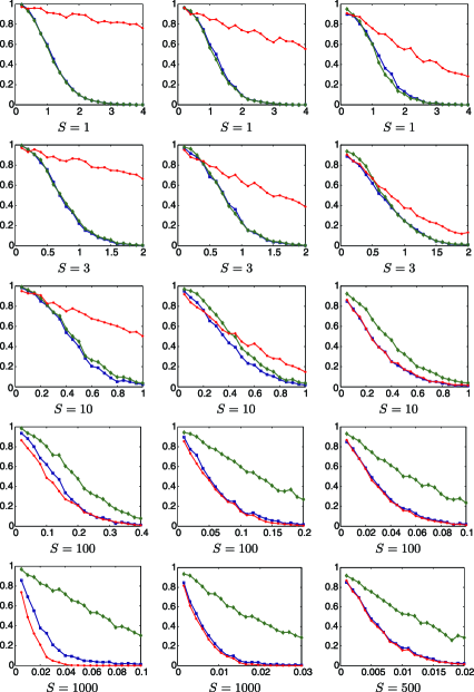
Figure 1: Left column: identity design with $p=10\mbox{,}000$. Middle column: Gaussian design with $p=10\mbox{,}000$ and $n=2\mbox{,}000$. Right column: Gaussian design with $p=10\mbox{,}000$ and $n=500$. Sparsity level $S$ is indicated below each plot. In each plot, the empirical risk (based on $1\mbox{,}000$ trials) of each method [ANOVA (red bullets); higher criticism (blue squares); Max test (green diamonds)] is plotted against $r$ (note the different scales).

We performed simulations with matrices of sizes $500\times 10\mbox{,}000$, $2\mbox{,}000\times 10\mbox{,}000$, $1\mbox{,}000\times 100\mbox{,}000$ and $5\mbox{,}000\times 100\mbox{,}000$, various sparsity levels, and strategically selected values of $r$. Each data point corresponds to an average over $1\mbox{,}000$ trials in the case where $p=10\mbox{,}000$, and over $500$ trials when $p=100\mbox{,}000$. A new design matrix is sampled for each trial. The performance of each of the three methods is computed in terms of its best (empirical) risk defined as the sum of probabilities of type I and II errors achievable across all thresholds. The results are reported in Figures 1 and 2. As expected, the detection thresholds for the Gaussian design are quite

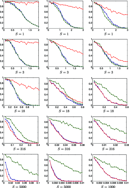
Figure 2: Left column: identity design with $p=100\mbox{,}000$. Middle column: Gaussian design with $p=100\mbox{,}000$ and $n=5\mbox{,}000$. Right column: Gaussian design with $p=100\mbox{,}000$ and $n=1\mbox{,}000$. Sparsity level $S$ is indicated below each plot. In each plot, the empirical risk (based on 500 trials) of each method [ANOVA (red bullets); higher criticism (blue squares); Max test (green diamonds)] is plotted against $r$ (note the different scales).

close to those available for the identity design. The performance of ANOVA improves very quickly as the sparsity decreases, dominating the Max test with $S=\sqrt{p}$; its performance also improves as $n$ becomes smaller, in accordance with (7). The performance of the Max test follows the opposite pattern, degrading as $S$ increases. Interestingly, the higher criticism remains competitive across the different sparsity levels.

6 Discussion

It is possible to extend our results to setups with correlated errors, with known covariance. As discussed in Section 1, suppose $\mathbf{z}$ in (4) is $\mathcal{N}({\mathbf{0}},\mathbf{V})$. We may then whiten the noise by multiplying both sides of (4) by $\mathbf{L}^{-1}$, where $\mathbf{L}\mathbf{L}^{T}$ is a Cholesky decomposition of $\mathbf{V}$. This leads to a model of the form

$$\mathbf{y}=\mathbf{L}^{-1}\mathbf{X}{\bolds\beta}+\mathbf{z},$$

which is our problem with $\mathbf{L}^{-1}\mathbf{X}$ instead of $\mathbf{X}$. In some situations, the noise covariance matrix may not be known and we refer to hj09 for a brief discussion of this issue.

Although several generalizations are possible, an interesting open problem is to determine the detection boundary for a given sequence of designs $\{\mathbf{X}_{n\times p}\}$ with $n$ and $p$ growing to infinity. We have seen that if most of the predictor variables are only weakly correlated, then the detection boundary is as if the predictors were orthogonal. Similar conclusions for certain types of square designs in which $n=p$ are also presented in the work of Hall and Jin hj09 . Although we introduced some sharp results in Section 4 corresponding to some important design matrices, the class of matrices for which we have definitive answers is still quite limited. We hope other researchers will engage this area of research and develop results toward a general theory.

References

- (1) {barticle}[mr] \bauthor\bsnmAkritas, \bfnmM. G.\binitsM. G. and \bauthor\bsnmPapadatos, \bfnmN.\binitsN. (\byear2004). \btitleHeteroscedastic one-way ANOVA and lack-of-fit tests. \bjournalJ. Amer. Statist. Assoc. \bvolume99 \bpages368–382. \biddoi=10.1198/016214504000000412, issn=0162-1459, mr=2062823 \bptokimsref \endbibitem
- (2) {bmisc}[auto:STB—2011/10/17—13:52:43] \bauthor\bsnmArias-Castro, \bfnmE.\binitsE., \bauthor\bsnmCandès, \bfnmE. J.\binitsE. J. and \bauthor\bsnmPlan, \bfnmY.\binitsY. \bhowpublishedSupplement to “Global testing under sparse alternatives: ANOVA, multiple comparisons and the higher criticism.” DOI:10.1214/11-AOS910SUPP. \bptokimsref \endbibitem
- (3) {barticle}[mr] \bauthor\bsnmBerman, \bfnmSimeon M.\binitsS. M. (\byear1964). \btitleLimit theorems for the maximum term in stationary sequences. \bjournalAnn. Math. Statist. \bvolume35 \bpages502–516. \bidissn=0003-4851, mr=0161365 \bptokimsref \endbibitem
- (4) {barticle}[mr] \bauthor\bsnmCandès, \bfnmEmmanuel J.\binitsE. J., \bauthor\bsnmRomberg, \bfnmJustin\binitsJ. and \bauthor\bsnmTao, \bfnmTerence\binitsT. (\byear2006). \btitleRobust uncertainty principles: Exact signal reconstruction from highly incomplete frequency information. \bjournalIEEE Trans. Inform. Theory \bvolume52 \bpages489–509. \biddoi=10.1109/TIT.2005.862083, issn=0018-9448, mr=2236170 \bptokimsref \endbibitem
- (5) {barticle}[mr] \bauthor\bsnmCandes, \bfnmEmmanuel J.\binitsE. J. and \bauthor\bsnmTao, \bfnmTerence\binitsT. (\byear2006). \btitleNear-optimal signal recovery from random projections: Universal encoding strategies? \bjournalIEEE Trans. Inform. Theory \bvolume52 \bpages5406–5425. \biddoi=10.1109/TIT.2006.885507, issn=0018-9448, mr=2300700 \bptokimsref \endbibitem
- (6) {barticle}[auto:STB—2011/10/17—13:52:43] \bauthor\bsnmCastagna, \bfnmJ. P.\binitsJ. P., \bauthor\bsnmSun, \bfnmS.\binitsS. and \bauthor\bsnmSiegfried, \bfnmR. W.\binitsR. W. (\byear2003). \btitleInstantaneous spectral analysis: Detection of low-frequency shadows associated with hydrocarbons. \bjournalThe Leading Edge \bvolume22 \bpages120–127. \bptokimsref \endbibitem
- (7) {barticle}[auto:STB—2011/10/17—13:52:43] \bauthor\bsnmChurchill, \bfnmG.\binitsG. (\byear2002). \btitleFundamentals of experimental design for cDNA microarrays. \bjournalNature Genetics \bvolume32 \bpages490–495. \bptokimsref \endbibitem
- (8) {barticle}[mr] \bauthor\bsnmDeo, \bfnmChandrakant M.\binitsC. M. (\byear1972). \btitleSome limit theorems for maxima of absolute values of Gaussian sequences. \bjournalSankhyā Ser. A \bvolume34 \bpages289–292. \bidissn=0581-572X, mr=0334319 \bptokimsref \endbibitem
- (9) {barticle}[mr] \bauthor\bsnmDonoho, \bfnmDavid\binitsD. and \bauthor\bsnmJin, \bfnmJiashun\binitsJ. (\byear2004). \btitleHigher criticism for detecting sparse heterogeneous mixtures. \bjournalAnn. Statist. \bvolume32 \bpages962–994. \biddoi=10.1214/009053604000000265, issn=0090-5364, mr=2065195 \bptokimsref \endbibitem
- (10) {barticle}[mr] \bauthor\bsnmDonoho, \bfnmDavid L.\binitsD. L. (\byear2006). \btitleCompressed sensing. \bjournalIEEE Trans. Inform. Theory \bvolume52 \bpages1289–1306. \biddoi=10.1109/TIT.2006.871582, issn=0018-9448, mr=2241189 \bptokimsref \endbibitem
- (11) {barticle}[mr] \bauthor\bsnmDonoho, \bfnmDavid L.\binitsD. L. and \bauthor\bsnmHuo, \bfnmXiaoming\binitsX. (\byear2001). \btitleUncertainty principles and ideal atomic decomposition. \bjournalIEEE Trans. Inform. Theory \bvolume47 \bpages2845–2862. \biddoi=10.1109/18.959265, issn=0018-9448, mr=1872845 \bptokimsref \endbibitem
- (12) {bmisc}[auto:STB—2011/10/17—13:52:43] \bauthor\bsnmDuarte, \bfnmM.\binitsM., \bauthor\bsnmDavenport, \bfnmM.\binitsM., \bauthor\bsnmWakin, \bfnmM.\binitsM. and \bauthor\bsnmBaraniuk, \bfnmR.\binitsR. (\byear2006). \bhowpublishedSparse signal detection from incoherent projections. In 2006 IEEE International Conference on Acoustics, Speech and Signal Processing, 2006. ICASSP 2006 Proceedings 3 III–III. \bptokimsref \endbibitem
- (13) {barticle}[mr] \bauthor\bsnmDudoit, \bfnmSandrine\binitsS., \bauthor\bsnmShaffer, \bfnmJuliet Popper\binitsJ. P. and \bauthor\bsnmBoldrick, \bfnmJennifer C.\binitsJ. C. (\byear2003). \btitleMultiple hypothesis testing in microarray experiments. \bjournalStatist. Sci. \bvolume18 \bpages71–103. \biddoi=10.1214/ss/1056397487, issn=0883-4237, mr=1997066 \bptokimsref \endbibitem
- (14) {barticle}[mr] \bauthor\bsnmEfron, \bfnmBradley\binitsB., \bauthor\bsnmTibshirani, \bfnmRobert\binitsR., \bauthor\bsnmStorey, \bfnmJohn D.\binitsJ. D. and \bauthor\bsnmTusher, \bfnmVirginia\binitsV. (\byear2001). \btitleEmpirical Bayes analysis of a microarray experiment. \bjournalJ. Amer. Statist. Assoc. \bvolume96 \bpages1151–1160. \biddoi=10.1198/016214501753382129, issn=0162-1459, mr=1946571 \bptokimsref \endbibitem
- (15) {bbook}[mr] \bauthor\bsnmFisher, \bfnmRonald A.\binitsR. A. (\byear1973). \btitleStatistical Methods for Research Workers, \bedition14th ed.—revised and enlarged. \bpublisherHafner, \baddressNew York. \bidmr=0346954 \bptokimsref \endbibitem
- (16) {barticle}[mr] \bauthor\bsnmGoeman, \bfnmJelle J.\binitsJ. J., \bauthor\bparticlevan de \bsnmGeer, \bfnmSara A.\binitsS. A. and \bauthor\bparticlevan \bsnmHouwelingen, \bfnmHans C.\binitsH. C. (\byear2006). \btitleTesting against a high dimensional alternative. \bjournalJ. R. Stat. Soc. Ser. B Stat. Methodol. \bvolume68 \bpages477–493. \biddoi=10.1111/j.1467-9868.2006.00551.x, issn=1369-7412, mr=2278336 \bptokimsref \endbibitem
- (17) {barticle}[mr] \bauthor\bsnmGribonval, \bfnmRémi\binitsR. and \bauthor\bsnmBacry, \bfnmEmmanuel\binitsE. (\byear2003). \btitleHarmonic decomposition of audio signals with matching pursuit. \bjournalIEEE Trans. Signal Process. \bvolume51 \bpages101–111. \biddoi=10.1109/TSP.2002.806592, issn=1053-587X, mr=1956096 \bptokimsref \endbibitem
- (18) {barticle}[mr] \bauthor\bsnmHall, \bfnmPeter\binitsP. and \bauthor\bsnmJin, \bfnmJiashun\binitsJ. (\byear2008). \btitleProperties of higher criticism under strong dependence. \bjournalAnn. Statist. \bvolume36 \bpages381–402. \biddoi=10.1214/009053607000000767, issn=0090-5364, mr=2387976 \bptokimsref \endbibitem
- (19) {barticle}[mr] \bauthor\bsnmHall, \bfnmPeter\binitsP. and \bauthor\bsnmJin, \bfnmJiashun\binitsJ. (\byear2010). \btitleInnovated higher criticism for detecting sparse signals in correlated noise. \bjournalAnn. Statist. \bvolume38 \bpages1686–1732. \biddoi=10.1214/09-AOS764, issn=0090-5364, mr=2662357 \bptokimsref \endbibitem
- (20) {bmisc}[auto:STB—2011/10/17—13:52:43] \bauthor\bsnmHaupt, \bfnmJ.\binitsJ. and \bauthor\bsnmNowak, \bfnmR.\binitsR. (\byear2007). \bhowpublishedCompressive sampling for signal detection. In IEEE Int. Conf. on Acoustics, Speech, and Signal Processing (ICASSP) 3 III-1509–III-1512. \bptokimsref \endbibitem
- (21) {bbook}[auto:STB—2011/10/17—13:52:43] \bauthor\bsnmHonig, \bfnmM.\binitsM. (\byear2009). \btitleAdvances in Multiuser Detection. \bpublisherWiley, \baddressHoboken, NJ. \bptokimsref \endbibitem
- (22) {barticle}[mr] \bauthor\bsnmIngster, \bfnmYu. I.\binitsY. I. (\byear1998). \btitleMinimax detection of a signal for -balls. \bjournalMath. Methods Statist. \bvolume7 \bpages401–428 (1999). \bidissn=1066-5307, mr=1680087 \bptnotecheck year\bptokimsref \endbibitem
- (23) {barticle}[mr] \bauthor\bsnmIngster, \bfnmYuri I.\binitsY. I., \bauthor\bsnmTsybakov, \bfnmAlexandre B.\binitsA. B. and \bauthor\bsnmVerzelen, \bfnmNicolas\binitsN. (\byear2010). \btitleDetection boundary in sparse regression. \bjournalElectron. J. Stat. \bvolume4 \bpages1476–1526. \biddoi=10.1214/10-EJS589, issn=1935-7524, mr=2747131 \bptokimsref \endbibitem
- (24) {barticle}[auto:STB—2011/10/17—13:52:43] \bauthor\bsnmJames, \bfnmD.\binitsD., \bauthor\bsnmClymer, \bfnmB. D.\binitsB. D. and \bauthor\bsnmSchmalbrock, \bfnmP.\binitsP. (\byear2001). \btitleTexture detection of simulated microcalcification susceptibility effects in magnetic resonance imaging of breasts. \bjournalJournal of Magnetic Resonance Imaging \bvolume13 \bpages876–881. \bptokimsref \endbibitem
- (25) {bmisc}[mr] \bauthor\bsnmJin, \bfnmJiashun\binitsJ. (\byear2003). \bhowpublishedDetecting and estimating sparse mixtures. Ph.D. thesis, Stanford Univ. \bptokimsref \endbibitem
- (26) {barticle}[auto:STB—2011/10/17—13:52:43] \bauthor\bsnmKerr, \bfnmM.\binitsM., \bauthor\bsnmMartin, \bfnmM.\binitsM. and \bauthor\bsnmChurchill, \bfnmG.\binitsG. (\byear2000). \btitleAnalysis of variance for gene expression microarray data. \bjournalJ. Comput. Biol. \bvolume7 \bpages819–837. \bptokimsref \endbibitem
- (27) {bbook}[mr] \bauthor\bsnmLedoux, \bfnmMichel\binitsM. (\byear2001). \btitleThe Concentration of Measure Phenomenon. \bseriesMathematical Surveys and Monographs \bvolume89. \bpublisherAmer. Math. Soc., \baddressProvidence, RI. \bidmr=1849347 \bptokimsref \endbibitem
- (28) {bbook}[mr] \bauthor\bsnmLehmann, \bfnmE. L.\binitsE. L. and \bauthor\bsnmRomano, \bfnmJoseph P.\binitsJ. P. (\byear2005). \btitleTesting Statistical Hypotheses, \bedition3rd ed. \bpublisherSpringer, \baddressNew York. \bidmr=2135927 \bptokimsref \endbibitem
- (29) {barticle}[mr] \bauthor\bsnmLemmens, \bfnmP. W. H.\binitsP. W. H. and \bauthor\bsnmSeidel, \bfnmJ. J.\binitsJ. J. (\byear1973). \btitleEquiangular lines. \bjournalJ. Algebra \bvolume24 \bpages494–512. \bidissn=0021-8693, mr=0307969 \bptokimsref \endbibitem
- (30) {bbook}[mr] \bauthor\bsnmMallat, \bfnmStéphane\binitsS. (\byear2009). \btitleA Wavelet Tour of Signal Processing: The Sparse Way, \bedition3rd ed. \bpublisherAcademic Press, \baddressAmsterdam. \bidmr=2479996 \bptnotecheck year\bptokimsref \endbibitem
- (31) {barticle}[auto:STB—2011/10/17—13:52:43] \bauthor\bsnmMallat, \bfnmS.\binitsS. and \bauthor\bsnmZhang, \bfnmZ.\binitsZ. (\byear1993). \btitleMatching pursuits with time-frequency dictionaries. \bjournalIEEE Trans. Signal Process. \bvolume41 \bpages3397–3415. \bptokimsref \endbibitem
- (32) {barticle}[mr] \bauthor\bsnmMathew, \bfnmThomas\binitsT. and \bauthor\bsnmSinha, \bfnmBimal Kumar\binitsB. K. (\byear1988). \btitleOptimum tests for fixed effects and variance components in balanced models. \bjournalJ. Amer. Statist. Assoc. \bvolume83 \bpages133–135. \bidissn=0162-1459, mr=0941007 \bptokimsref \endbibitem
- (33) {barticle}[auto:STB—2011/10/17—13:52:43] \bauthor\bsnmMcCarthy, \bfnmM.\binitsM., \bauthor\bsnmAbecasis, \bfnmG.\binitsG., \bauthor\bsnmCardon, \bfnmL.\binitsL., \bauthor\bsnmGoldstein, \bfnmD.\binitsD., \bauthor\bsnmLittle, \bfnmJ.\binitsJ., \bauthor\bsnmIoannidis, \bfnmJ.\binitsJ. and \bauthor\bsnmHirschhorn, \bfnmJ.\binitsJ. (\byear2008). \btitleGenome-wide association studies for complex traits: Consensus, uncertainty and challenges. \bjournalNature Reviews Genetics \bvolume9 \bpages356–369. \bptokimsref \endbibitem
- (34) {bmisc}[auto:STB—2011/10/17—13:52:43] \bauthor\bsnmMeng, \bfnmJ.\binitsJ., \bauthor\bsnmLi, \bfnmH.\binitsH. and \bauthor\bsnmHan, \bfnmZ.\binitsZ. (\byear2009). \bhowpublishedSparse event detection in wireless sensor networks using compressive sensing. In 43rd Annual Conference on Information Sciences and Systems (CISS), 2009 181–185. \bptokimsref \endbibitem
- (35) {bbook}[mr] \bauthor\bsnmMontgomery, \bfnmDouglas C.\binitsD. C. (\byear2009). \btitleDesign and Analysis of Experiments, \bedition7th ed. \bpublisherWiley, \baddressHoboken, NJ. \bidmr=2552961 \bptokimsref \endbibitem
- (36) {bbook}[mr] \bauthor\bsnmPiantadosi, \bfnmSteven\binitsS. (\byear2005). \btitleClinical Trials: A Methodologic Perspective, \bedition2nd ed. \bpublisherWiley, \baddressHoboken, NJ. \biddoi=10.1002/0471740136, mr=2154988 \bptokimsref \endbibitem
- (37) {barticle}[auto:STB—2011/10/17—13:52:43] \bauthor\bsnmSlonim, \bfnmD.\binitsD. (\byear2002). \btitleFrom patterns to pathways: Gene expression data analysis comes of age. \bjournalNature Genetics \bvolume32 \bpages502–508. \bptokimsref \endbibitem
- (38) {barticle}[mr] \bauthor\bsnmStrohmer, \bfnmThomas\binitsT. and \bauthor\bsnmHeath, \bfnmRobert W.\binitsR. W., Jr. (\byear2003). \btitleGrassmannian frames with applications to coding and communication. \bjournalAppl. Comput. Harmon. Anal. \bvolume14 \bpages257–275. \biddoi=10.1016/S1063-5203(03)00023-X, issn=1063-5203, mr=1984549 \bptokimsref \endbibitem
- (39) {barticle}[auto:STB—2011/10/17—13:52:43] \bauthor\bsnmWiller, \bfnmC.\binitsC., \bauthor\bsnmSanna, \bfnmS.\binitsS., \bauthor\bsnmJackson, \bfnmA.\binitsA., \bauthor\bsnmScuteri, \bfnmA.\binitsA., \bauthor\bsnmBonnycastle, \bfnmL.\binitsL., \bauthor\bsnmClarke, \bfnmR.\binitsR., \bauthor\bsnmHeath, \bfnmS.\binitsS., \bauthor\bsnmTimpson, \bfnmN.\binitsN., \bauthor\bsnmNajjar, \bfnmS.\binitsS. and \bauthor\bsnmStringham, \bfnmH.\binitsH. et al. (\byear2008). \btitleNewly identified loci that influence lipid concentrations and risk of coronary artery disease. \bjournalNature Genetics \bvolume40 \bpages161–169. \bptokimsref \endbibitem
- (40) {barticle}[auto:STB—2011/10/17—13:52:43] \bauthor\bsnmZhang, \bfnmG.\binitsG., \bauthor\bsnmZhang, \bfnmS.\binitsS. and \bauthor\bsnmWang, \bfnmY.\binitsY. (\byear2000). \btitleApplication of adaptive time-frequency decomposition in ultrasonic NDE of highly-scattering materials. \bjournalUltrasonics \bvolume38 \bpages961–964. \bptokimsref \endbibitem