Modeling the near-UV band of GK stars, Paper I: LTE models

Abstract

We present a grid of LTE atmospheric models and synthetic spectra that cover the spectral class range from mid-G to mid-K, and luminosity classes from V to III, that is dense in $T_{\rm eff}$ sampling ($\Delta T_{\rm eff}=62.5$ K), for stars of solar metallicity and moderately metal poor scaled solar abundance ($[{{\rm A}\over{\rm H}}]=0.0$ and $-0.5$). All models have been computed with two choices of atomic line list: a) the “big” line lists of Kurucz (1992a) that best reproduce the broad-band solar blue and near UV $f_{\lambda}$ level, and b) the “small” lists of Kurucz & Peytremann (1975) that provide the best fit to the high resolution solar blue and near-UV spectrum. We compare our model SEDs to a sample of stars carefully selected from the large catalog of uniformly re-calibrated spectrophotometry of Burnashev (1985) with the goal of determining how the quality of fit varies with stellar parameters, especially in the historically troublesome blue and near-UV bands. We confirm that our models computed with the “big” line list recover the derived $T_{\rm eff}$ values of the PHOENIX NextGen grid, but find that the models computed with the “small” line list provide greater internal self-consistency among different spectral bands, and closer agreement with the empirical $T_{\rm eff}$ scale of Ramirez & Melendez (2005), but not to the interferometrically derived $T_{\rm eff}$ values of Baines et al. (2010). We find no evidence that the near UV band discrepancy between models and observations for Arcturus ($\alpha$ Boo) reported by Short & Hauschildt (2003) and Short & Hauschildt (2009) is pervasive, and that Arcturus may be peculiar in this regard.

1 Introduction

Critical comparisons of the observed absolute spectral energy distribution (SED), $f_{\lambda}(\lambda)$, to that predicted with PHOENIX computational models from the near UV to the red have been carried out for the Sun, Procyon, and Arcturus (see Short & Hauschildt (2009), Short & Hauschildt (2005), and Short & Hauschildt (2003)). They presented evidence that both LTE and non-LTE models increasingly over-predict the $f_{\lambda}$ level for $\lambda<4000$ Å  as the $T_{\rm eff}$ value of the star decreases from that of early G stars to that of early K. The investigations to date have been restricted to bright standard stars for which there is very high quality spectroscopic and spectrophotometric data, with the consequence that the quality of the SED fit has not been well sampled in the stellar parameter space $T_{\rm eff}/\log g/{\rm[}{{\rm A}\over{\rm H}}{\rm]}$. Here, we take the first major step to rectify the situation by comparing a large grid of model SEDs spanning the cool side of the HR diagram to observed SEDs taken from the spectrophotometric catalog of Burnashev (1985). Our goal is to map out the goodness of fit, and the magnitude of any systematic discrepancies between model and observed SEDs as a function of the three stellar parameters, $T_{\rm eff}$, $\log g$, and [${{\rm A}\over{\rm H}}$], with the more fundamental goal of constraining the physical character of the sources of any discrepancies. We also compare our $T_{\rm eff}$ values inferred from SED fitting to other empirical and theoretical $T_{\rm eff}$ calibrations.

2 Observed $f_{\lambda}(\lambda)$ distributions

Burnashev (1985) presented a large catalog (henceforth B85) of observed SEDs taken with photo-electric instruments on 0.5m class telescopes at various observatories in the former USSR from the late 1960s to the mid 1980s and uniformly photometrically re-calibrated to the “Chilean system” (Short & Hauschildt (2009) contains a more detailed description of the individual data sources included in this compilation). These data sets all generally cover the $\lambda$ range 3200 to 8000 Å  with $\Delta\lambda=25$ Å, and have a quoted “internal photometric accuracy” of $\approx 3.5\%$.

We have harvested from the B85 catalog a sample of stars that meet the following criteria: 1) having an entry in the 5^th Revised Edition of the Bright Star Catalogue (Hoffleit & Warren, 1991), (henceforth BSC5), 2) having a spectral class later than G0 and earlier than M0, 3) having a luminosity class in the range from V to III, 4) having an entry in the metallicity catalog of Cayrel et al. (2001), 5) having no variability, chemical peculiarity, or binarity flags in BSC5, and 6) having an $f_{\lambda}$ distribution that was not obviously inconsistent based on visual inspection, with those of other stars of the same BSC5 spectral class and within $\pm 1$ sub-class. The spectral and luminosity classes were taken from The Revised Catalog of MK Spectra Types for the Cooler Stars (Keenan & Newsom, 2000), the paper of Keenen & Barnbaum (1999), or The Perkins Catalog of Revised MK Types for the Cooler Stars Keenan & McNeil (1989), in decreasing order of preference. For nine objects without spectral classes determined by Keenan or his collaborators, we took spectral types from the General Catalogue of Stellar Spectral Classifications (Version 2010-Mar) Skiff (2010): HD 50522 (Abt, 2008), HD 147675 (Torres et al., 2006), (Houk & Cowley, 1975), HD 71878 (Gray et al., 2006), HD 222107 (Gray et al., 2003), HD 221673 (Abt, 1981), HD 156266, 115383 (Harlan, 1974), HD 34559, 49878 (Adams et al., 1935). For the six objects for which Skiff (2010) had multiple conflicting spectral classes, we took the class that agreed with that listed in BSC5. Application of criterion 6) necessitated only including stars for which there was more than one object of the same spectral class, to within $\pm 0.5$ sub-classes. We found that application of these six criteria, along with the metallicity criteria described below, limited us to 33 stars of spectral class ranging from G5 to K4 for giants and G0 to G5 for dwarfs. All spectra were corrected for their heliocentric radial velocity, RV, using the RV values in BSC5. However, we expect the RV correction to have a very minor effect on the quality of spectral fitting at the low spectral resolution of the B85 data.

We restricted the sample to two metallicity ranges based on the value of [${{\rm A}\over{\rm H}}$] reported in the catalog of Cayrel et al. (2001): a) stars of $-0.1<[{{\rm A}\over{\rm H}}]<0.1$, and b) stars of $-0.4<[{{\rm A}\over{\rm H}}]<-0.6$. These two ranges are expected to contain stars of measured [${{\rm A}\over{\rm H}}$] approximately equal to 0.0 and -0.5, respectively, on the grounds that the quoted uncertainties, $\Delta[{{\rm A}\over{\rm H}}]$, of determinations of overall metallicity typically have quoted uncertainties of the order of $\pm 0.1$. For stars that contained multiple entries in the catalog of Cayrel et al. (2001), we based the metallicity selection on either the mean, or the median, value of [${{\rm A}\over{\rm H}}$], depending on whether there were obvious outlier values and skew. Metallicity range b) approximately represents a moderately metal poor population typical of the older thick disk, represented by stars such as Arcturus ([${{\rm A}\over{\rm H}}$]$\approx-0.7$). Stars of [${{\rm A}\over{\rm H}}$]$<-0.5$ are increasingly rare in B85 catalog as [${{\rm A}\over{\rm H}}$] decreases, so -0.5 was the lowest [${{\rm A}\over{\rm H}}$] value for which we could harvest a significant number of stars of [${{\rm A}\over{\rm H}}$] value within $\pm 0.1$ of each other. Applying the six criteria described above, we harvested 30 and 3 stars from the B85 catalog in each of the metallicity ranges a) and b), respectively. Table 1 contains the list of the stars that were selected in each metallicity range, and the number of [${{\rm A}\over{\rm H}}$] measurements in the Cayrel et al. (2001) catalog. Some stars had two independently measured SEDs in the B85 catalog, and where that is the case, both spectra are included in our analysis and provide a check on the internal consistency of the B85 spectrophotometry. The number of spectra is also indicated in Table 1.

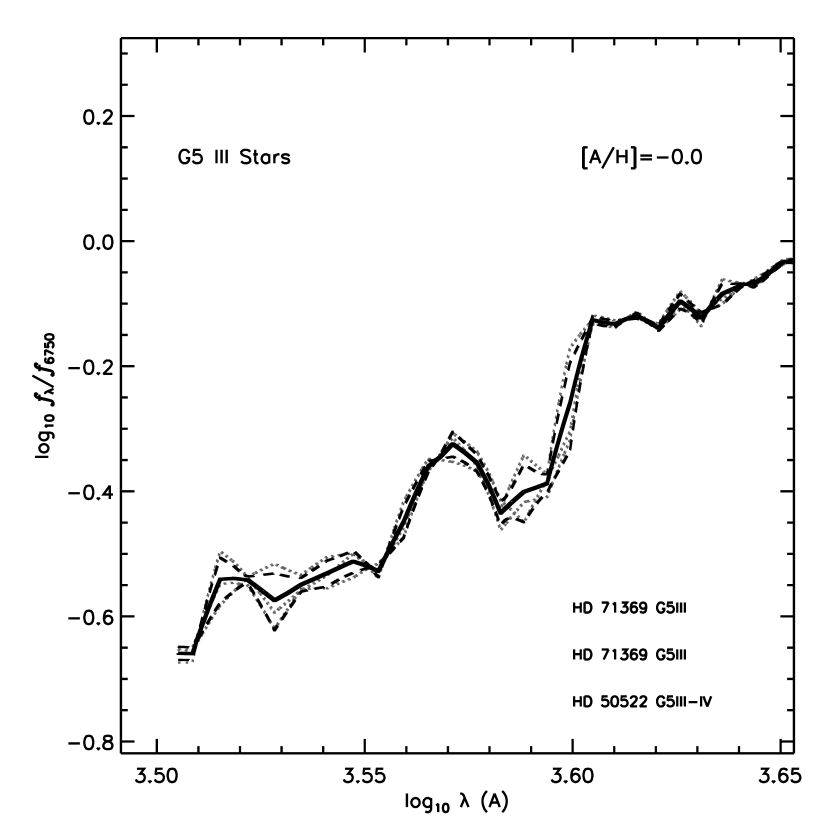
Figure 2: G5 III sample (two stars, three spectra). Light gray dotted lines: individual normalized stellar spectra, $f_{\lambda,{\rm 6750}}$ (see text), from catalog of B85; black solid line: sample average $f_{\lambda,{\rm 6750}}$ spectrum; black dashed lines: $\pm 1~{}\sigma$ $f_{\lambda,{\rm 6750}}$ spectra.

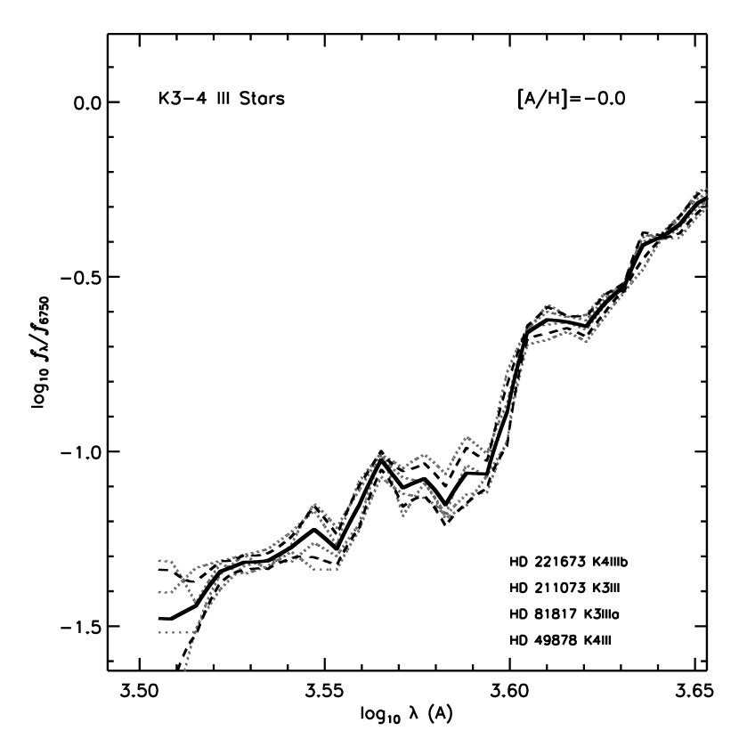
Figure 3: Same as Fig. 2, but for the K3-4 III sample (four stars, four spectra).

Figs. 2 and 3 show, for the hottest and coolest giant samples, the individual spectra of all stars of that sample, over-plotted with the sample mean spectrum and the spectra of the $\pm 1\sigma$ deviation from the mean. Note that the $\sigma$ values are most clearly meaningful for the two samples that contain more than a few spectra, namely, the G8 III and K0 III stars of solar metallicity. For most samples, the spectra that passed our selection procedure fall within $\pm 1\sigma$ of the mean at most $\lambda$ values. We have separately calculated mean and deviation spectra for each sub-sample.

2.1 K0 III sample

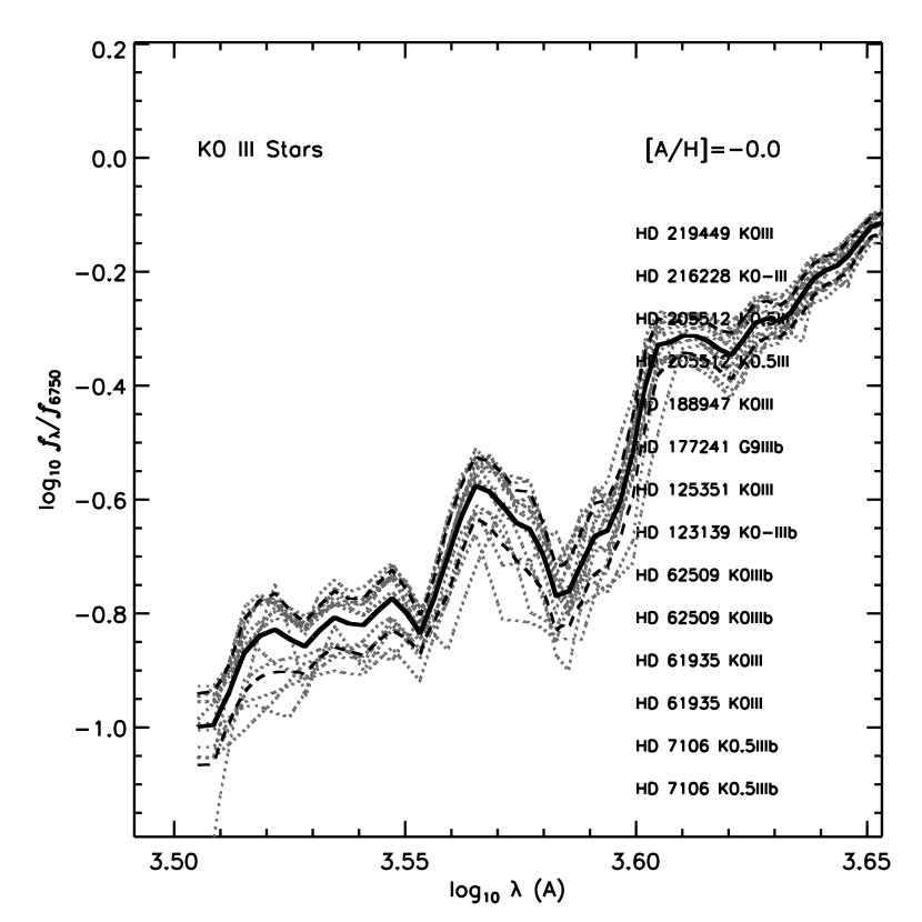
Figure 4: Same as Fig. 2, but for the K0 III sample (ten stars, fourteen spectra). The spectra fall into two groups in the $3.50<\log\lambda<3.58$ range, those of “high” and those of “low” UV flux, with an apparent dearth of stars of intermediate UV flux level.

The K0 III sample, shown in Fig. 4 is special in that it contains more spectra than the other sub-classes (14 spectra of ten objects), and the distribution of spectra has a bifurcation that can be most clearly seen in the $\log\lambda$ region from 3.52 to 3.55 (3300 to 3550 Å). Therefore, we have broken up the K0 III sample into two sub-samples, an $l$ sub-sample of four stars (six spectra) with “low”, and an $h$ sub-sample with six stars (eight spectra) with “high”, UV $f_{\lambda}$ level, respectively. The stars belonging to the $l$ and $h$ sub-samples are indicated in Table 1. This bifurcation may be an artifact of our sorting of stars with an effective precision of about one spectral sub-class. Around K0, stars can be typed to half-sub-class precision (see, for example, Keenan & Newsom (2000)), and differences of $\approx 0.5$ spectral sub-classes would presumably have the greatest effect in the blue and near UV spectral bands. We note that two of the four stars in our “low” sample have a spectral class of K0.5 III.

2.2 Arcturus

To compare with the results of Short & Hauschildt (2003), it is necessary to include Arcturus ($\alpha$ Boo. HD124897) (and other stars of the same SED, were they available), in the current investigation. The metallicity catalog of Cayrel et al. (2001) lists 17 measurements of [${{\rm A}\over{\rm H}}$] for Arcturus ranging from -0.370 to -0.810, with most values in the range of -0.4 to -0.6, and the average being -0.54. Arcturus is the only star in the B85 catalog with a spectral class in the range from K0 to K2 III with measured $[{{\rm A}\over{\rm H}}]$ values within $\pm 0.2$ dex of -0.5. Therefore, we cannot form a K1 III sample at $[{{\rm A}\over{\rm H}}]\approx-0.5$ for quality control inspection, or for forming a mean spectrum, as we have with the other spectral classes and metallicities. Moreover, Arcturus is flagged in BSC5 as being chemically peculiar, with the spectral class designation being K1.5IIIFe-0.5.

With an apparent $V$ band magnitude of -0.04, the B85 spectrophotometric data for Arcturus should be of relatively high quality. The B85 catalog contains three measured $f_{\lambda}$ distributions, two of which are consistent with each other on the basis of visual inspection. The third is higher by about 0.05 dex for $\log\lambda$ less than about 3.55 ($\lambda<3550$ Å). We have formed a sample at spectral class K1.5 III for stars of nominal $[{{\rm A}\over{\rm H}}]$ equal to -0.5 using these three SEDs.

3 Model grid

3.1 Atmospheric structure calculations

We have computed a grid of about 400 atmospheric models under the approximation of LTE with spherical $1D$ geometry spanning a range in $T_{\rm eff}$ from 6250 to 4000 K with a sampling, $\Delta T_{\rm eff}$, of 125 K, and in $\log g$ from 1.5 to 5.0 with a sampling of 0.5, for [${{\rm A}\over{\rm H}}$] values of 0.0 and -0.5. A $\Delta T_{\rm eff}$ interval of 125 K is close to the nominal $T_{\rm eff}$ difference between successive spectral sub-classes among GK stars (see, for example, Ramirez & Melendez (2005)). Furthermore, we interpolate in our synthetic spectrum grid to achieve an effective $\Delta T_{\rm eff}$ of 62.5 K, as described below.

For spherical models, a value of the effective radius, $R_{\rm eff}$, at $\tau_{\rm 12000}=1$ is also required as input. However, we expect the value of $R_{\rm eff}$ will have a minor impact on the computed SED compared to $T_{\rm eff}$, $\log g$, and [${{\rm A}\over{\rm H}}$], and we used values corresponding to a mass of $1M_{\rm Sun}$ at the given value of $\log g$ for all models. Because we are restricted to stars in the spectral class range G5 to K5, most of which are of luminosity class III (see Section 2), we expect the mass distribution of the progenitor main sequence objects to be of the order of $1M_{\rm Sun}$. Hauschildt et al. (1999b) found that for supergiant models of given $T_{\rm eff}$ and $\log g$, which are even more spherically extended than our models. the choice of mass in the range 2.5 to 7.5 $M_{\rm Sun}$ lead to only small differences in the relative SED.

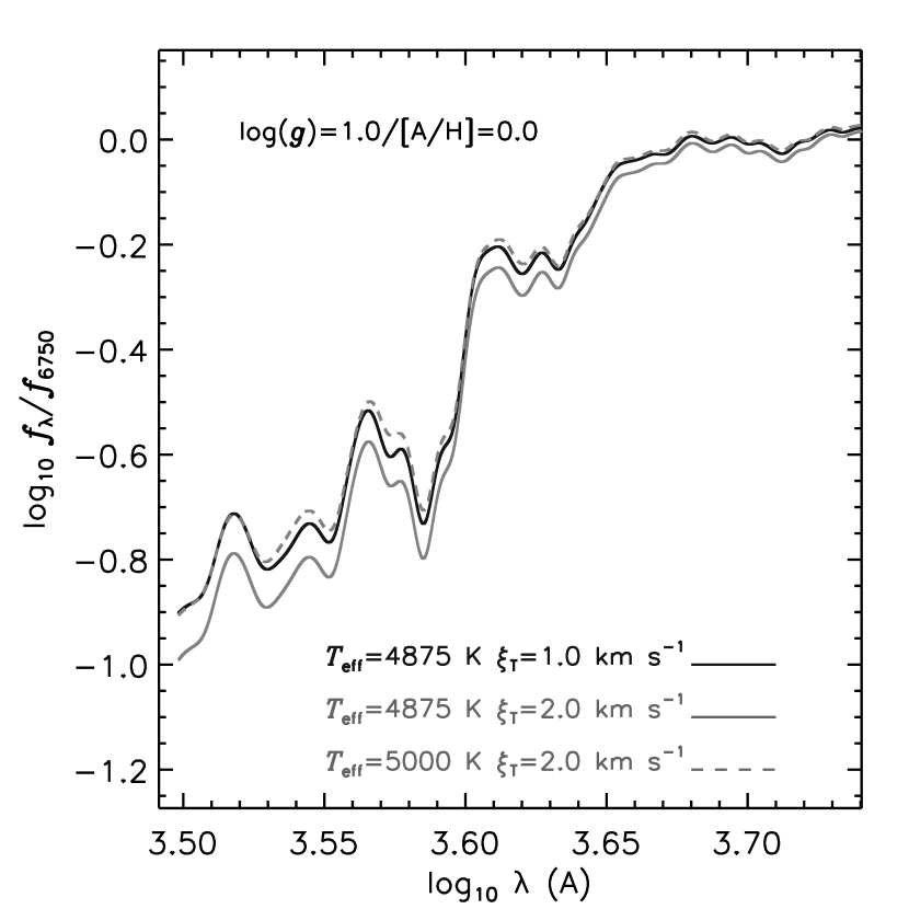
Figure 1: Synthetic SEDs for models of varying $T_{\rm eff}$ and $\xi_{\rm T}$ for $\log g=2.0$ and $[{{\rm A}\over{\rm H}}]=0.0$. Solid dark line: model of $T_{\rm eff}=4875$ K and $\xi_{\rm T}=1.0$ km s^-1, solid light line: model of $T_{\rm eff}=4875$ K and $\xi_{\rm T}=2.0$ km s^-1, dashed line: model of $T_{\rm eff}=5000$ K and $\xi_{\rm T}=2.0$ km s^-1.

The observed SED will depend on the value adopted for the micro-turbulent velocity dispersion, $\xi_{\rm T}$, which determines the extent to which spectral lines are blended in crowded spectral regions, such as the blue band, and therefore, affects the $f_{\lambda}$ level to different extents in different $\lambda$ regions. We adopted values of 1.0 and 2.0 km s^-1 for $\log g$ values greater than and less than 3.5, respectively. Short & Hauschildt (2005) found that $\xi_{\rm T}=1$ km s^-1 provided a good fit to the solar SED from the near UV to the red. From analysis of line profiles in high resolution high $S/N$ spectra of G and K III stars, previous investigators have found $\xi_{\rm T}$ ranging from 1.5 to 2.0 km s^-1 (Gray, 1982), (Foy, 1978), (Gustafsson et al., 1974). In Fig. 1 we compare two synthetic SEDs computed with $\xi_{\rm T}=1$ and $2$ km s^-1 for a model of $T_{\rm eff}=4875$ K, $\log g=2.0$, and [${{\rm A}\over{\rm H}}$]=0.0, and a model of $\xi_{\rm T}=2$ km s^-1 and the same stellar parameters except that $T_{\rm eff}$ is 5000 K. The value of $\xi_{\rm T}$ makes an increasingly large difference as $\lambda$ decreases because of the increasing density of spectral absorption lines, and reaches a maximum of $\approx 0.1$ dex at 3200 Å. This is a significant effect, and a proper exploration of the effect on the stellar parameters determined from SED fitting will require a model grid with a $\xi_{\rm T}$ dimension, and is beyond the scope of the current investigation. However, we can note qualitatively from Fig. 1 that models models in which $\xi_{\rm T}$ is over-estimated by 1 km s^-1 will produce fits to the blue and near UV band flux level that over-estimate the value of $T_{\rm eff}$ by $\approx 100$ K. For all models, we adopted a mixing length parameter for the treatment of convective flux transport of one pressure scale height.

For all models, we adopt scaled solar abundances. There is evidence that mildly metal poor stars of [${{\rm A}\over{\rm H}}$]$=-0.5$ have abundance distributions that are enhanced in $\alpha$-elements with respect to the Sun by 0.2 to 0.3 dex (see, for example, Peterson et al. (1993)). However, given the scope of the model grid required for this initial investigation, we have decided to restrict ourselves to scaled solar ${{\rm A}\over{\rm H}}$ distributions. There has been recent controversy over the values of the solar abundances for important elements such as CNO, with Asplund et al. (2004) and other papers in that Series, revising the values downward by 0.2 to 0.3 dex on the basis of $3D$ models that account for hydrodynamic turbulence. However, the work of Asplund et al. (2004) has been found to be discrepant with abundances determined from very sensitive helioseismological fitting, and has recently been thrown into question on the grounds of self-consistency (see, for example, the very thorough recent investigation by Pinsonneault & Delahaye (2009)). For simplicity, we restrict ourselves in this investigation to the solar abundance distribution of Grevesse et al. (1992).

For each grid point, we compute two models that differ from each other in the choice of atomic line list. Our Series 1 and 2 models use the “big” and “small” line lists of Short & Hauschildt (2009), respectively, and that paper contains a description of the content of the two line lists, the evidence for and against each one, and an investigation of the effect that the choice of line list has on the computed SED, especially in the heavily line blanketed blue and near UV region. Short & Hauschildt (2009) found that the choice of “big” or “small” line list has a significant impact on the computed $f_{\lambda}$ values in the blue and near UV bands for both the Sun and Arcturus, and concluded that NLTE models of the Sun with the “big” line list provide a better fit to the measured $f_{\lambda}$ distribution of Neckel & Labs (1984), but that those with the “small” line list provide a better fit to three other measured $f_{\lambda}$ distributions, including one measured from space. Therefore, we have decided to evaluate the fit provided by models with both choices of line list here. We note that the choice of line list affects the model structure as well as directly affecting the synthetic SED calculation.

3.2 Synthetic spectra

For each model in both Series 1 and 2 we computed self-consistent synthetic spectra in the $\lambda$ range 3000 to 8000 Å  with a spectral resolution ($R={\lambda\over\Delta\lambda}\approx 350\,000$) to ensure that spectral lines were adequately sampled. These were then degraded to match the low resolution measured $f_{\lambda}$ distributions of B85 by convolution with a Gaussian kernel. B85 present their data with a sampling of 25 Å, but, neither B85, nor any of the original source publications that are still accessible, describe the instrumental spectral profile. Based on trial comparisons of observed SEDs with synthetic $f_{\lambda}$ spectra convolved with Gaussians of various FWHM values, we found that a Gaussian instrumental profile with a FWHM value of 75 Å  provided the closest qualitative match to the spectral structure in the observed SEDs. Therefore, we have convolved all our synthetic spectra with a normalized Gaussian kernel of FWHM equal to 75 Å. We note that this convolution also automatically accounts for macro-turbulence, which has been found to be around 5.0 km s^-1 for G and K II stars Gray (1982). We interpolate in $\log T_{\rm eff}$ between pairs of synthetic SEDs to obtain a grid with an effective sampling, $\Delta T_{\rm eff}$, of 62.5 K. A $T_{\rm eff}$ difference of 62.5 K at 3300 Å  corresponds to a difference in the $\log f_{\lambda}$ of a blackbody of 0.07, and this difference will be smaller for larger $\lambda$ and higher $T_{\rm eff}$ values. For comparison, the discrepancy in near UV band $\log f_{\lambda}$ level between LTE models and observations found by Short & Hauschildt (2009) for Arcturus around 3300 Å  is $\approx 0.15$.

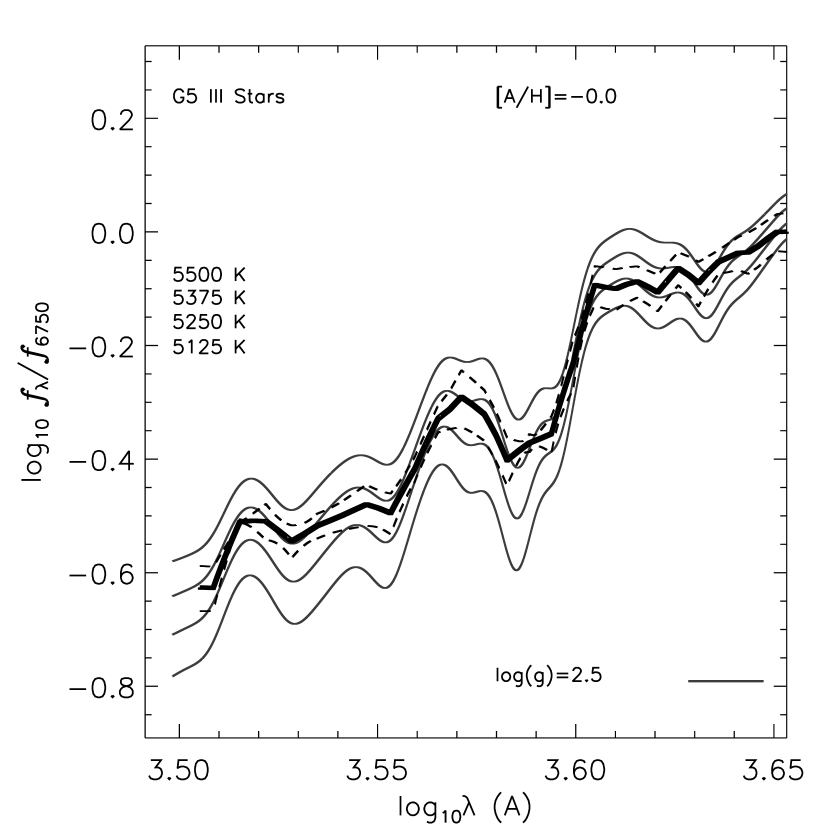
Figure 5: G5 III sample: Comparison of sample average to synthetic $f_{\lambda,{\rm 6750}}$ spectra of Series 1 models. Solid black line: sample average $f_{\lambda,{\rm 6750}}$ spectrum, black dashed lines: $\pm 1~{}\sigma$ spectra, solid gray lines: closest matching and bracketing synthetic $f_{\lambda,{\rm 6750}}$ spectra.

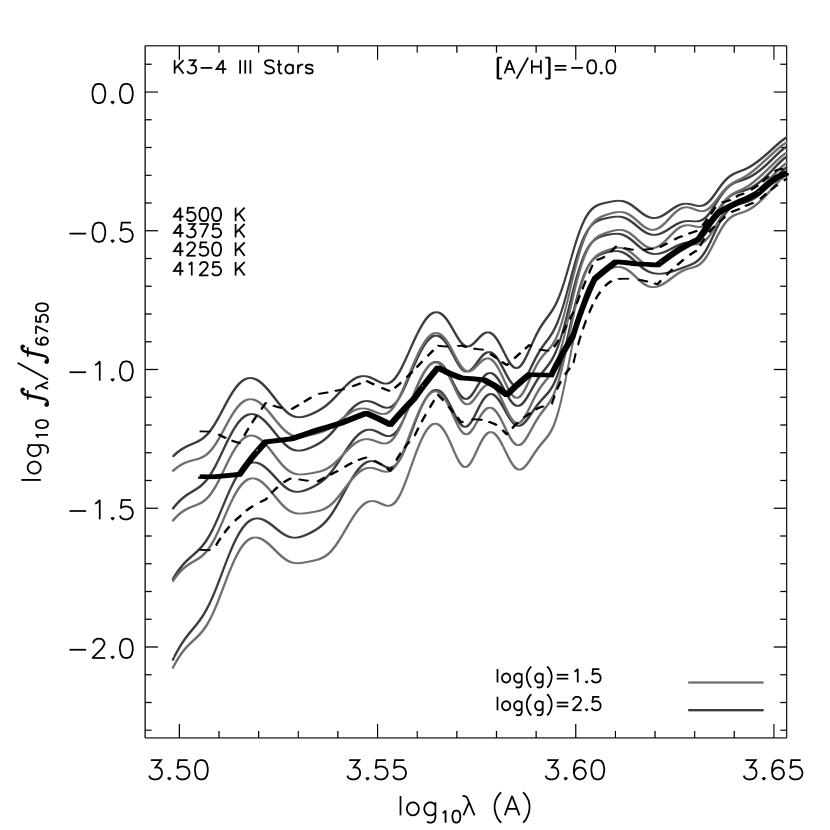
Figure 6: Same as Fig. 5, but for the K3-4 sample. Medium gray lines: $\log g=2.5$, light gray lines: $\log g=1.5$. For clarity, the synthetic spectra of the $\log g=2.0$ models have been omitted.

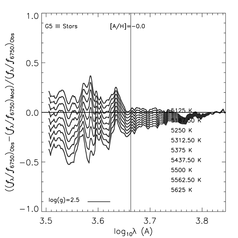
Figure 7: G5 III sample - Spectra of the relative difference between the observed sample average $f_{\lambda,{\rm 6750}}$ spectrum and synthetic $f_{\lambda,{\rm 6750}}$ spectra of Series 1 models. The horizontal line indicates a difference of zero. The vertical line represent the break-point between the “blue” and “red” bands.

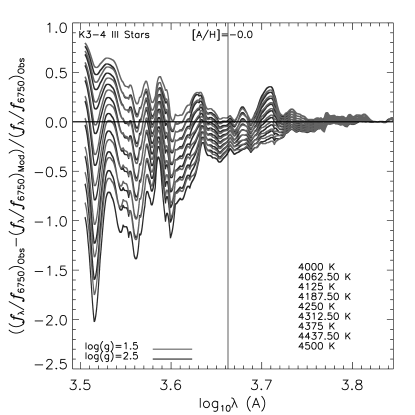
Figure 9: Same as Fig. 7, but for the K3-4 sample. Black lines: $\log g=2.5$, gray lines: $\log g=1.5$. For clarity, the synthetic spectra the $\log g=2.0$ models have been omitted.

All spectra, observed and synthetic, have been normalized by dividing by the average of their flux in the 6600 to 6900 Å  region, chosen to be just blue of the first significant telluric contamination bands due to O₂ and H₂O, to produce the distribution denoted $f_{\lambda,{\rm 6750}}={f_{\lambda}\over f_{\lambda}(\lambda={\rm 6750})}$. Figs. 5 and 6 show the comparison of the mean and $\pm 1\sigma$ spectra of the observed $f_{\lambda,{\rm 6750}}$ distributions with the closest matching and bracketing synthetic $f_{\lambda,{\rm 6750}}$ distributions for the hottest and coolest giant samples. Figs. 7 and 9 show the difference between the mean of the observed $f_{\lambda,{\rm 6750}}$ distribution and the closest matching and bracketing synthetic distributions relative to the observed mean distribution, $(f_{\lambda,{\rm 6750,MeanObserved}}-f_{\lambda,{\rm 6750,Model}})/f_{\lambda,{\rm 6750,MeanObserved}}$ for the same two samples.

4 Goodness of fit statistics

We interpolate all observed and synthetic spectra onto a uniform $\lambda$ grid of $\Delta\lambda=0.01$ Å  that moderately over-samples all spectra at all $\lambda$ values, and compute for each spectral class sample the root mean square relative deviation, $\sigma$, of the mean observed $f_{\lambda,{\rm 6750}}$ distribution from the closest matching and bracketing synthetic $f_{\lambda,{\rm 6750}}$ distributions in the $\lambda$ range from 3200 to 7000 Å, according to

$$\sigma^{2}={1\over N}\sum_{i}^{N}((f_{\lambda,{\rm 6750,Obs}}-f_{\lambda,{\rm 6750,Mod}})/f_{\lambda,{\rm 6750,Obs}})^{2}$$ (1)

where $N$ is the number of $\lambda$ points in the $\lambda$ grid in the 3200 to 7000 Å  range.

We also compute separate RMS values, $\sigma_{\rm blue}$ and $\sigma_{\rm red}$, for the so-called “blue” and “red” sub-ranges of 3200 to 4600 Å  and 4600 to 7000 Å, respectively. We also compute the mean relative deviations, $\Delta_{\rm blue}$ and $\Delta_{\rm red}$, for the two sub-ranges, according to.

$$\Delta={1\over N}\sum_{i}^{N}(f_{\lambda,{\rm 6750,Obs}}-f_{\lambda,{\rm 6750,Mod}})/f_{\lambda,{\rm 6750,Obs}}$$ (2)

A comparison of the blue and red $\sigma$ values indicates how well the synthetic spectra fit in the blue and near UV band given the quality of fit in the red band. The comparison of $\Delta$ between the bands allows an assessment of systematic discrepancies throughout the blue compared to the red because, unlike $\sigma$, $\Delta$ retains its sign. A break-point of 4600 Å  was chosen on the basis of visual inspection of where the deviation of the synthetic from the observed spectrum starts to become rapidly larger as $\lambda$ decreases. In Tables 2 and 3 we present the $\sigma$, $\sigma_{\rm blue}$, and $\sigma_{\rm red}$ values for the Series 1 and 2 models, respectively, along with the best fit value of $T_{\rm eff}$ and $\log g$ for each star. The value of the model $[{{\rm A}\over{\rm H}}]$ is also tabulated, although, its value was specified a priori rather than fitted.

4.1 Trend with $T_{\rm eff}$

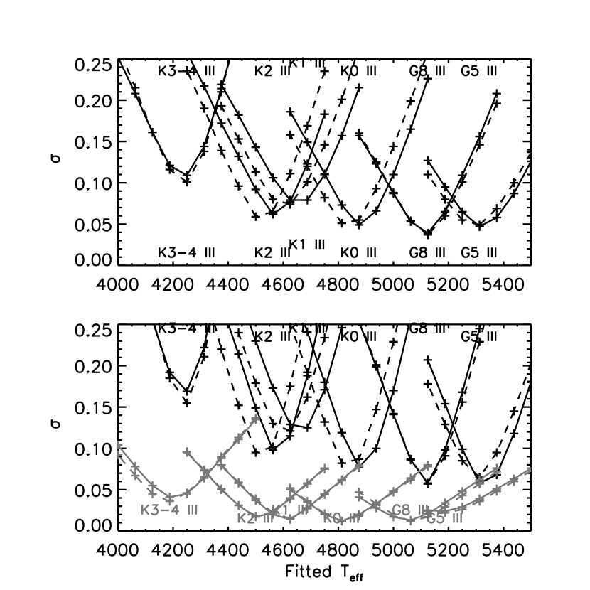
Figure 10: Giants of solar metallicity: Variation of $\sigma$ with model $T_{\rm eff}$. Solid line: Series 1 models; dashed line: Series 2 models. Upper panel: Fit to total SED; Lower panel: Black lines: fit to blue band; gray lines: fit to red band.

Fig. 10 shows the variation of $\sigma$, $\sigma{\rm blue}$, and $\sigma_{\rm red}$ with model $T_{\rm eff}$ for the giant stars of solar metallicity. The best fit $\sigma$ value generally increases with increasing lateness of the spectral class. We note that the density of spectral lines generally increases with increasing lateness. Therefore, this trend in the discrepancy between synthetic and observed SEDs could be explained by inadequacies is the input atomic data for bound-bound ($b-b$) transitions, or by inadequacies in the treatment of spectral line formation. The best fit $\sigma$ values for the Series 1 and 2 models differ negligibly for the earlier spectral classes, and there is marginal evidence that the Series 2 models provide a slightly better fit (lower $\sigma$ value) for the latest spectral classes.

4.1.1 G5 III sample

The behavior of the variation of $\sigma_{\rm red}$ with $T_{\rm eff}$ for the G5 III stars is peculiar and leads to a spurious result for the best fitted value of $T_{\rm eff}$. From Fig. 7 it can be seen that this is caused by a broad absorption feature exhibited by the observed SED with respect to the model SEDs ranging from a $\log\lambda$ value of 3.753 to 3.774 (5660 to 5940 Å). As a result, the value of $\sigma_{\rm red}$ is increased significantly, even for models that provide a good match to the overall spectrum. Therefore, our best fit value of $T_{\rm eff}$ for the G5 III models is best determined from the blue band alone. This deficit of absorption in the synthetic SEDs with respect to the observed ones is consistently present in the individual observed spectra for the G5 III stars, spans 12 data points in the raw observed spectrum, and varies smoothly with wavelength over a range of  280 Å. Therefore, it is likely caused by a cluster of spectral lines that are either missing, or are too weak, in the model spectra. We note that this discrepancy is either absent, or much less pronounced, in both the G4-5 V and G8 III stars, so appears to be localized in both $T_{\rm eff}$ and $\log g$.

We have examined histograms of the average numbers of spectral lines per Å  by atomic chemical species in a synthetic spectrum of a model of $T_{\rm eff}$/$\log g$/[${{\rm A}\over{\rm H}}$]=5250/2.5/0.0, representative of the models that fit the observed G5 III SED. We compared three $\lambda$ ranges: the problematic 5660 to 5940 Å  range, and the bracketing ranges of 5000 to 5660 and 5940 to 7000 Å. All three ranges show approximately the same pattern and same absolute average numbers of lines per unit wavelength for all atomic species that contribute a significant number of lines. We are unable to identify any suspect chemical species for which there is an excess or dearth of lines in the 5660 to 5940 region compared to neighboring regions that might provide a clue to the cause of the discrepancy.

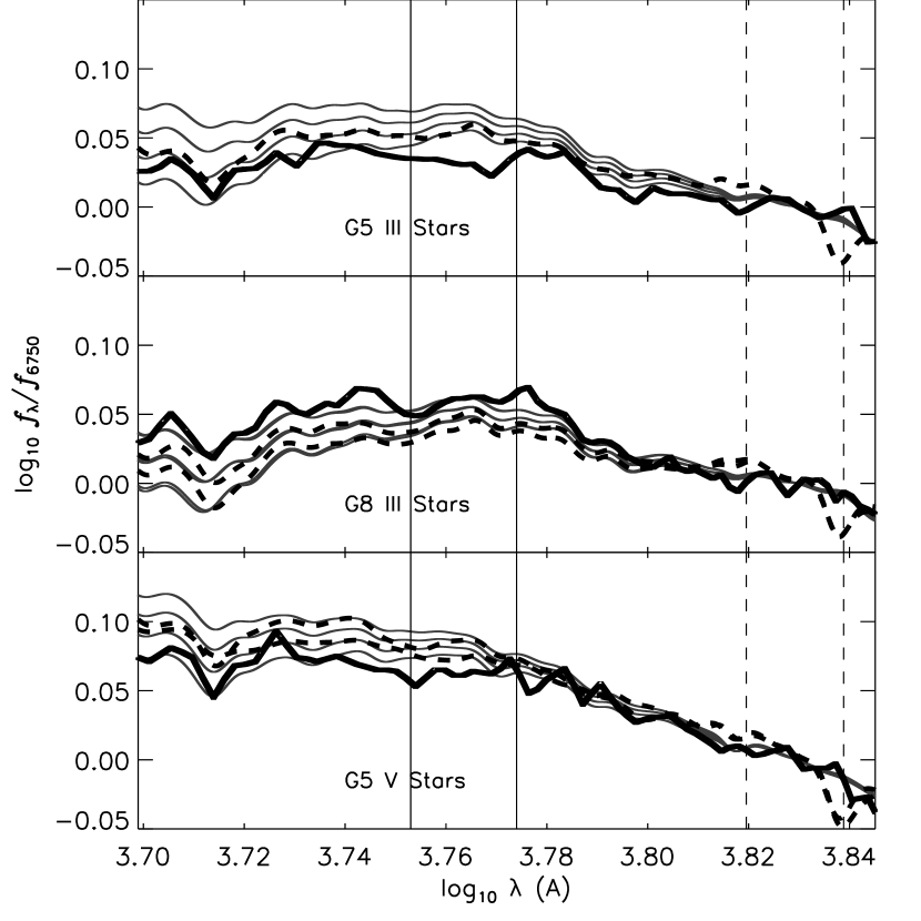
Figure 8: Comparison of B85 and Jacoby et al. (1984) observed spectra. Solid black line: sample mean from the B85 catalog as in Fig. 2. solid gray lines: synthetic spectra as in Figs. 5 and 6, dashed black lines: spectra from library of Jacoby et al. (1984) for a G5 III star (BD+281885, upper panel), a G7 (HD 249240) and a G8 (HD 245389) III star (middle panel), and a G4 (TR A 14) and a G6 (HD 22193) V star (lower panel). Vertical lines: solid: region of discrepancy between the B85 and PHOENIX spectra for G5 III stars; dashed: normalization region.

We have compared our mean observed spectra based on the B85 catalog for the G5 III and V, and G8 III types to representative spectra from the stellar spectrophotometric library of Jacoby et al. (1984). In Fig. 8 we show the comparison in the $\lambda$ range around the region of the G5 III discrepancy. The Jacoby et al. (1984) library does not have a spectrum for type G5 V, so we have compared our spectrum of that class to spectra for classes G4 and 6 V. The G4 V star is designated ’TR A 14’ and Jacoby et al. (1984) flag it as a star that could not be identified. However, for lack of an alternative, we use it as a comparison. There are small systematic differences between our mean B85 spectra and those of Jacoby et al. (1984) over a broad range of $\lambda$ for all three spectral types. However, for the G5 III sample, the Jacoby et al. (1984) spectrum is distinctly brighter than our mean B85 spectrum in the $\log\lambda$ 3.753 to 3.774 range, as compared the the bracketing $\log\lambda$ ranges, and is in greater agreement with our synthetic SED. We conclude that there may have been a data acquisition or calibration problem with the spectra in the B85 catalog that is very particular to the G5 III class. From Fig. 8 it can be seen that the B85 and Jacoby et al. (1984) spectra are much more consistent with each other throughout this region for the G5 V and G8 III classes. We note again that our B85 G5 III sample suffers from small-number statistics in that it consists of three spectra of two stars. In what we follows we only draw conclusions for the blue spectral band of the G5 III sample. (A full systematic comparison of our B85 mean spectra with those Jacoby et al. (1984) throughout our $\lambda$ range is beyond the scope of this investigation, but, the comparison in Fig. 8 is generally encouraging.)

4.1.2 Red vs blue band

For all samples, the best fit to the red band has a $\sigma$ value that is lower than that of the fit to the blue band by 0.05 to 0.1. This may partly reflect that all spectra were normalized to a common relative flux value in the red band (6750 Å). However, from Figs. 7 and 9 it can be seen that the difference spectra show increasing variability around the zero line in addition to any systematic trend away from the zero line. This indicates that the quality of the fit to the mean observed spectrum worsens with decreasing $\lambda$ regardless of how the observed and synthetic spectra were normalized. For all solar metallicity giants, the Series 1 models fitted to the blue band consistently give best fit $T_{\rm eff}$ values that are one $\Delta T_{\rm eff}$ resolution element, 63K, higher than those fitted to the red. For the Series 2 models, both bands yield the same best fit $T_{\rm eff}$ value for the K0 to K2 III stars, whereas for the two ends of the $T_{\rm eff}$ range where both bands can be used, G8 and K3-4, the Series 2 models lead to the same pattern as the Series 1 modes, with the blue band fit yielding a higher $T_{\rm eff}$ value. This may provide marginal evidence that the Series 2 models lead to a greater consistency of fit throughout the SED.

4.1.3 Series 1 vs Series 2

For the samples at the two ends of our $T_{\rm eff}$ range, G5 to G8 and K3-4, fits with the Series 1 and 2 models both lead to the same value of inferred $T_{\rm eff}$, to within the $\Delta T_{\rm eff}$ precision of the grid. However, for the intermediate samples, K0 to K2, the Series 2 models fitted to the blue and to the overall SED consistently lead to fitted $T_{\rm eff}$ values that are one $\Delta T_{\rm eff}$ resolution element lower than that of the Series 1 models. Because the Series 2 models have less line blanketing, they predict greater flux in the blue with respect to the red than do the Series 1 models. Therefore, we expect them to yield lower fitted $T_{\rm eff}$ values to a given observed SED.

4.2 Trend with $\log g$

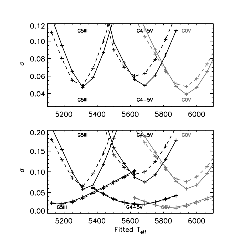
Figure 11: Same as Fig. 10, but for the dwarf stars.

Fig. 11 shows the fitting quantities for the G5 III, G4-5 V, and G0 V stars of solar metallicity. Examination of these figures allows a limited assessment of how the quality of fit varies in the $\log g$ dimension at spectral class G5. The Series 1 models provide fits of similar quality to the total SED of G5 stars of both luminosity classes, III and V. By contrast, the Series 2 models provide a significantly worse fit to the class V than to the class III stars, with the quality of fit to class III differing negligibly from that provided by the Series 1 models. Furthermore, we note that this same discrepancy in the quality of fit provided by Series 1 and 2 is also seen for the G0 V stars. Fig. 11 shows that these trends in the quality of the fit to the total band is driven mainly by the quality of fit to the blue band. The suggestion is that the models computed with the “big” input line list provide a better fit to the blue band spectra of dwarfs than, and as good a fit to the giants as, the models computed with the “small” line list.

For the G4-5 V stars, the $T_{\rm eff}$ value fitted to the blue band with Series 1 models is 63 K higher than that fitted with Series 2 models, whereas, for the G 5 III stars, both Series yield the same blue band $T_{\rm eff}$ value. The G4-5 V stars are anomalous among our solar metallicity stars in that the Series 2 models give a higher fitted $T_{\rm eff}$ value to the red band than to the blue band. Unfortunately, our ability to compare the fit to the red band as a function of $\log g$ is undermined by the peculiarities with modeling the red band of the G5 III sample discussed earlier in this section.

4.3 Trend with [${{\rm A}\over{\rm H}}$]

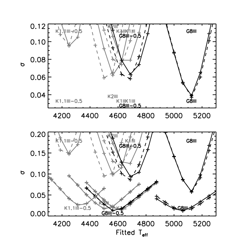
Figure 12: Same as Fig. 10, but for the metal poor giants.

Fig. 12 shows the same quantities for the G8 III and K1 to K2 III stars of [${{\rm A}\over{\rm H}}$] equal to 0.0 and -0.5, and allows a limited assessment of how the quality of fit varies in the metallicity dimension. For a given spectral class, both the Series 1 and 2 models provide a significantly better quality of fit to the stars of solar metallicity than to those that are metal poor. This may in part reflect the inappropriateness of scaled solar abundance models for fitting the population of stars of [${{\rm A}\over{\rm H}}$]$=-0.5$. By contrast, for a given $T_{\rm eff}$ value, there is some evidence that all models provide a similar quality of fit, independent of [${{\rm A}\over{\rm H}}$]. We note that the metal-poor G8 III star has a best fit $T_{\rm eff}$ value closer to that of the solar metallicity K1 to K2 stars than that of the solar metallicity G8 III star, and the value of $\sigma$ for the red and blue bands, and for the overall SED, is similar for the G8 III/[${{\rm A}\over{\rm H}}$]$=-0.5$ and K2 III/[${{\rm A}\over{\rm H}}$]$=0.0$ stars. This suggests that the strongest relation is the anti-correlation between $T_{\rm eff}$ and $\sigma$ rather than that between [${{\rm A}\over{\rm H}}$] and $\sigma$.

4.4 Arcturus

For the Arcturus sample (K1.5 III, [${{\rm A}\over{\rm H}}$]$=-0.5$) the $T_{\rm eff}$ value fitted to the red band is higher than that fitted to the blue by 63 K. Therefore, models fitted to the red band would predict too much flux in the blue and near UV bands. This is consistent with the results of Short & Hauschildt (2003) and Short & Hauschildt (2009), who also compared models to the observed $f_{\lambda}$ distribution of B85. We note that 62.5 K is the numerical precision of our $T_{\rm eff}$ grid. Therefore, the most we can conclude is that the discrepancy in the best fit $T_{\rm eff}$ value between the red and blue bands is in the range of 31 to 125 K. By contrast, the solar metallicity giants of spectral type G8 to K4 do not show this trend, having best fit $T_{\rm eff}$ values that are lower by 63 K in the red band (to within the precision of our model grid). Moreover, our only other metal poor sample, G8 III, also shows the opposite trend as Arcturus, with a red band $T_{\rm eff}$ value that is 125 K (two $\Delta T_{\rm eff}$ increments) lower than that of the blue band. The suggestion is that Arcturus may be peculiar among giants generally in that models fitted to the red over-predict the blue band flux.

5 Comparison to other $T_{\rm eff}$ calibrations

5.1 Empirical calibration

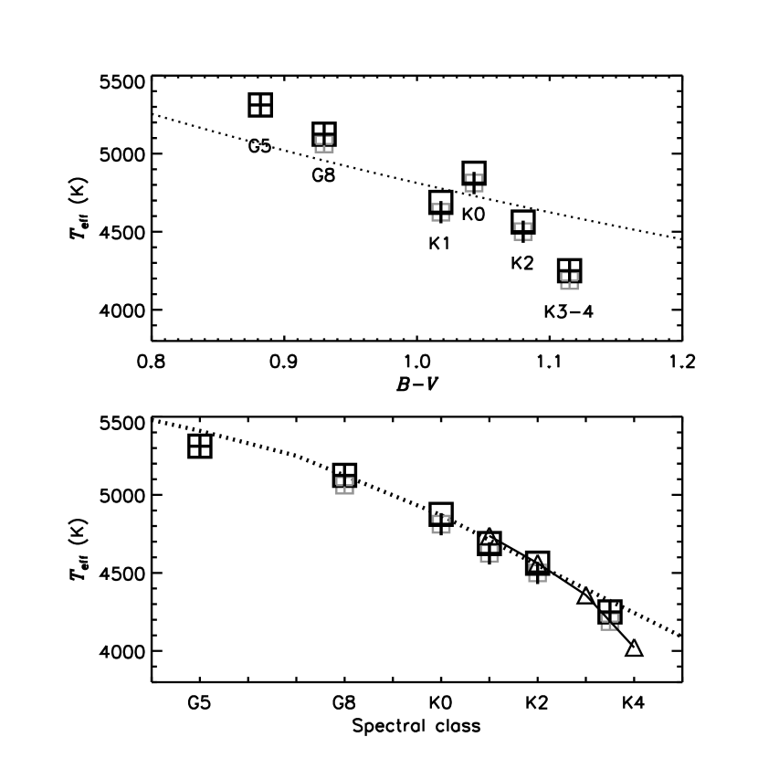
Figure 13: Comparison of our best fit $T_{\rm eff}$ values with other $T_{\rm eff}$ calibrations. Squares: Series 1 models; Crosses: Series 2 models. Black symbols: Fit to the blue band; Gray symbols: fit to the red band. Dotted lines: Upper panel: Empirical calibration of RM05; Lower panel: PHOENIX NextGen models fitted to stellar spectral libraries (BBCR04). Triangles (lower panel): $T_{\rm eff}$ values of B10.

Ramirez & Melendez (2005) (RM05) present an empirical determination of $T_{\rm eff}$ based on applying the Infrared Flux Method (IRFM) to 100 dwarfs and giants of spectral class from F0 to K5 and $[{{\rm A}\over{\rm H}}]$ from -4 to +0.4 as a function of many observables, including Johnson $B-V$ color. This work is an extension of the definitive $T_{\rm eff}$ calibration work of Alonso et al. (1999) and other papers in that series. They quote standard deviations of 30 to 120 K, and find that their IRFM $T_{\rm eff}$ scale agrees to within 10 K with directly determined values for stars with measured angular diameters. RM05 do not present $T_{\rm eff}$ as a function of spectral class. However, we have computed mean and RMS ($\sigma$) $B-V$ values for each of our spectral class samples using colors for individual objects from the Catalogue of Homogeneous Means in the UBV System (Mermilliod, 1991). We then used the fitted Eqs., 1 and 2, and the fitting co-efficients of Tables 1 and 2, of RM05 to interpolate in $B-V$ and produce empirical $T_{\rm eff}$ values for each of our spectral class samples and metallicities. We checked our interpolated $T_{\rm eff}$ values against, presumably, less accurate values found from linear interpolation in Tables 4 and 5 of RM05 and found them to be consistent. In Table 4 and Figs. 13 through 15 we present a comparison of our $T_{\rm eff}$ values fitted to our blue and red spectral ranges, and those of the RM05 calibration. Because of the peculiarities of fitting the red band of the G5 III stars described in section 4, the red band $T_{\rm eff}$ value has been suppressed in Figs. 13 through 15.

Baines et al. (2010) (B10) used the CHARA array to interferometrically measure the angular diameters of 25 K giants in the $K$ band, including eight in the spectral class range K0 to K4 III with $[{{\rm A}\over{\rm H}}]$ values within $\pm 0.1$ of 0.0, and two in the K1 to 2 III range with $[{{\rm A}\over{\rm H}}]$ values within $\pm 0.1$ of -0.5. They combined their angular diameter measurements with distances from Hipparcos and photometrically inferred bolometeric flux values to derive $T_{\rm eff}$ values. We have calculated averages for their $T_{\rm eff}$ values for solar metallicity giants of spectral class K1 (three stars), K2 (two stars), K3 (1 star) and K4 (2 stars), and include these values in Table 4 and Fig. 13. They also present a measured $T_{\rm eff}$ value for an Arcturus analog (HD 170693, K1.5III-0.5). These results were published just as we were completing our investigation, so we included them for comparison. Unfortunately, none of the B10 stars are in the samples we selected from the B85 catalog.

5.1.1 Solar metallicity giants

For the G8 to K1 stars, the models of both series fitted to the red band give $T_{\rm eff}$ values closest to the RM05 values, and are consistently higher than RM05 by less than 100 K. For the K2 sample, our red band fit matches the RM05 value to within the $\pm 62.5$ K precision of our grid. The Series 1 models fitted to the blue band consistently yield $T_{\rm eff}$ values that are higher than the RM05 $T_{\rm eff}$ calibration. An equivalent alternate interpretation is that the Series 1 models with the RM05 $T_{\rm eff}$ value for their observed $B-V$ color would predict too little blue band flux compared to the observed SED, while providing a closer match to the red band.

The B10 $T_{\rm eff}$ values for classes K1 and 2 III are is closest agreement with our Series 1 values derived from the blue band, being an exact match at K2 III to within the precision of the respective values. Their value for the K3-4 stars is lower than our lowest value by $\approx 50$ K.

5.1.2 Solar metallicity dwarfs

For the G0 V stars, the Series 2 models fitted to the red band give a $T_{\rm eff}$ value very close to the RM05 value. All models fitted to the blue band give $T_{\rm eff}$ values that are too high by $\approx 100$ K. For the G4-5 stars all models give $T_{\rm eff}$ values that are consistent with each other, but 100 to 150 K higher than that of RM05. These results are similar to those found for G5 III stars in the blue band, so the discrepancy between our blue band $T_{\rm eff}$ scale and that of RM05 at spectral class G5 seems to be independent of $\log g$ in the 2.5 to 4.5 range,

5.1.3 Metal poor giants

For the G8 III stars of $[{{\rm A}\over{\rm H}}]=-0.5$, the Series 1 and 2 models fitted to the blue band provide a very close match to the $T_{\rm eff}$ value of RM05, better than the fit to the solar metallicity G8 giants. All models fitted to the red band provide $T_{\rm eff}$ values that are 100 to 150 K lower than that of RM05. For Arcturus (K1.5III-0.5), all models fitted to the red band give $T_{\rm eff}$ values in close agreement with RM05, being lower by 20 K. This result is consistent with our result for solar metallicity K1 and 2 stars, and suggests that the quality of our fit to the red band for early K giants is independent of metallicity in this [${{\rm A}\over{\rm H}}$] range. The B10 value for their one K1.5 III star of $[{{\rm A}\over{\rm H}}]=-0.5$ (HD 170693) is 75 K higher than our highest value.

5.2 Previous PHOENIX calibration

Bertone et al. (2004) (BBCR04) derived $T_{\rm eff}$ values from fitting theoretical SEDs for models of $[{{\rm A}\over{\rm H}}]=0.0$ taken from the NextGen grid computed with an earlier version of PHOENIX (V10) (Hauschildt et al., 1999b), The most important differences between V10 and V15 that are relevant to these models are 1) Improvements in the treatment of the line profiles so that many weak to moderate strength lines that were treated as Gaussian are now treated with Voigt profiles, and 2) Improvement in the quality of a wide variety of EOS input data. (Hauschildt et al., 1999a) to SEDs of solar metallicity dwarfs and giants of spectral class from early A to mid-M taken from the observational spectral libraries of Gunn & Stryker (1983) and Jacoby et al. (1984). We note that the NextGen models were computed using the “big” atomic line list of our Series 1 models. Among the main differences between the NextGen grid and the one presented here are: 1) the NextGen models of $\log g>3.5$ are computed with plane-parallel geometry, however, the effects of sphericity are expected to be negligible for that surface gravity range. 2) the NextGen models have the value of $\xi_{\rm T}$ set to 2 km s^-1 throughout the grid, independent of $\log g$. As discussed above, our value of $\xi_{\rm T}$ decreases to 1 km s^-1 for the dwarfs on the basis of our experience modeling the disk integrated flux spectrum of the Sun (Short & Hauschildt, 2005). BBCR04 do not provide an interpolation formula for $T_{\rm eff}$, so we have interpolated linearly in their Table 1 to find $T_{\rm eff}$ values for our spectral classes that are missing from their table. Table 4 and Figs. 13 through 15 include a comparison the $T_{\rm eff}$ values of BBCR04.

5.2.1 Solar metallicity giants

Generally, the BBCR04 $T_{\rm eff}$ scale is 50 to 150 K hotter than the empirical RM05 scale in our spectral class range, and our models fitted to the red band consistently provide $T_{\rm eff}$ values that are lower than those of BBCR04 by $\approx 50$ K. We note that our Series 1 models fitted to the blue band provide consistently very good agreement to the NextGen $T_{\rm eff}$ scale. That the Series 1 models would provide better agreement is expected since they are based on the same atomic line list as the NextGen grid, and the blue band is expected to show greater sensitivity to the treatment of line opacity than the red band. All of our fitted $T_{\rm eff}$ values are lower than the BBCR04 value for the earliest spectral class, G5 III, which implies that the BBCR04 $T_{\rm eff}$ scale would be even more discrepant with the empirical RM05 scale than ours is at the hot end of the sequence.

5.2.2 Dwarfs and metal poor stars

Again, for the G4-5 V stars, our Series 1 models fitted to the line-sensitive blue bands provide the closest match to the NextGen $T_{\rm eff}$ value, which is what we expect. Somewhat surprisingly, for the G0V star all our models yield $T_{\rm eff}$ values that are 200 to 250 K lower than of the NextGen models. This result is surprising in that we expect discrepancies due to inconsistencies and inaccuracies in the treatment of line blanketing, among other modeling aspects, to be reduced with increasing $T_{\rm eff}$. We do not find such a gross discrepancy at G0 V with the empirical RM05 $T_{\rm eff}$ scale.

6 Conclusions

Our giant sequence samples $T_{\rm eff}$ well from spectral class G5 to K3-4. The $\sigma$ value of the best fit to the giant star spectra for all spectral bands increases with later spectral class, with the value for the overall SED increasing from $\approx 0.05$ at spectral class G8 III to $\approx 0.10$ at spectral class K3-4 III. The quality of fit to the red band (4600 to 7000 Å) is significantly better than that to the blue (3200 to 4600 Å), with the best fit $\sigma$ value being $\approx$ 0.02 for classes G8 to K2 III. (Unfortunately, a peculiar discrepancy between the observed and synthetic spectra unique to the G5 III sample prevents us from meaningfully including that sample in conclusions drawn for the red band.) Higher best fit $\sigma$ values are driven by an increasing variation around zero in spectra of the difference between observed and synthetic spectra as $\lambda$ decreases, and correlates with the increasing density of spectral lines in $f_{\lambda}$ spectra with decreasing $\lambda$. Therefore, the contrast between the best fit $\sigma_{\rm blue}$ and $\sigma_{\rm red}$ values probably reflects inadequacies in the input atomic line list and/or the treatment of line formation.

For the Series 1 models, there is also a systematic effect with wavelength in that best fit models to the blue band yield a fitted $T_{\rm eff}$ value that is one $\Delta T_{\rm eff}$ grid resolution element (63 K) higher than those fit to the red band. Equivalently, models fitted to the red band will predict too little flux in the blue band. This result is in stark contrast to the results of Short & Hauschildt (2003) and Short & Hauschildt (2009), who found that models fitted to the red band of Arcturus (K1.5 III) predicted too much blue band flux. We note that our Series 1 models fitted to the blue band provide $T_{\rm eff}$ values that are within 50 K of the values derived with the PHOENIX NextGen grid, which also used the “big” atomic line list.

The Series 2 models (“small” line list) fitted to the blue band lead to best fit $T_{\rm eff}$ values for the early K giants that are 63 K lower than do the Series 1 models (“large” line list), thus providing greater consistency of best fit $T_{\rm eff}$ value among the spectral bands than do the Series 1 models. By contrast, for the two spectral classes for which we have reliable dwarf spectra, G0 and G4-5, the Series 1 models provide a better fit to the blue band of the dwarfs than those of Series 2, while the two Series provide an equally good fit to the red band of dwarfs. We conclude that there is marginal evidence that the Series 2 models provide a better fit to solar metallicity giants while Series 1 models provide a better fit to solar metallicity dwarfs.

When comparing giants of the same spectral class, the models provide a better fit at solar metallicity than at [${{\rm A}\over{\rm H}}$]$=-0.5$, However, when comparing giants of the same $T_{\rm eff}$ value, the models give a similar quality of fit at both metallicities. Taking into account the metallicity dependence in the $T_{\rm eff}$ calibration of the spectral classes, we conclude that the quality of fit provided by our models is not dependent, or only weakly dependent, on [${{\rm A}\over{\rm H}}$] in the range -0.5 to 0.0.

We find that Arcturus is peculiar among our stars in that it is the only object for which the best fit $T_{\rm eff}$ value to the blue band is lower than that for the red band, by 63 K. This result is qualitatively consistent with that of Short & Hauschildt (2003) and Short & Hauschildt (2009), who found that models fit to the yellow and red bands of Arcturus yielded significantly more blue and near UV band flux than observed. Those authors concluded that there is an important source of near UV band continuous opacity missing from cool star atmospheric models. One goal of this work was to determine the extent to which this discrepancy was pervasive among late type stars. We conclude that it is not, and that Arcturus may be peculiar in this regard. If anything, there is a tendency for models fit to spectra of all other spectral classes to under-predict the blue flux with respect to the red.

For the solar metallicity giants, we find that the Series 2 models, which yield consistent $T_{\rm eff}$ values between the red and blue bands, agree to within 100 K with the RM05 empirical $T_{\rm eff}$ values for our full range of spectral classes. For the K2 to K4 III stars, we recover the RM05 $T_{\rm eff}$ values to within the $\Delta T_{\rm eff}$ resolution of our model grid. The agreement of the Series 2 $T_{\rm eff}$ values with the RM05 values for the G0 and G4-5 V stars is also very good. For the metal poor giants, the relative success of Series 1 and 2 models is mixed with G8 and K1.5 III stars having contrasting results. By contrast, the very recently published interferometric $T_{\rm eff}$ values of B10 are in very close agreement to the Series 1 models fit to the blue band for early K giants. We conclude on balance that the Series 2 models (“small” atomic line list) provide greater internal self-consistency and agreement with empirical $T_{\rm eff}$ scale. We advise that the large atomic line lists containing many theoretically predicted lines of Fe-group elements be used with caution.

PHOENIX includes continuous molecular opacity from H₂, H${}_{\rm 2}^{\rm+}$, H${}_{\rm 2}^{\rm-}$ and MgH. Kurucz et al. (1987) found that including the photo-dissociation opacity of CH makes a detectable difference to the predicted flux of the Sun in a localized region around 4000 Å. Their calculations did not include the effect of line blanketing, so it is difficult to judge how detectable the difference is. Nevertheless, because molecules become increasingly important as $T_{\rm eff}$ decreases it would be worthwhile investigating the role of this opacity source in our models. In any case, Short & Hauschildt (2009) found that the continuous opacity in the Sun and Arcturus in the $\lambda\lambda 3000$ to $4000$ region is dominated, variously, by by H^- $b-f$, the combined $b-f$ opacity due to metals, the combined $f-f$ opacity of Mg and Si, and Thomson scattering, and the cross-sections for most of these are kown accurately enough that their dominance is not in doubt.

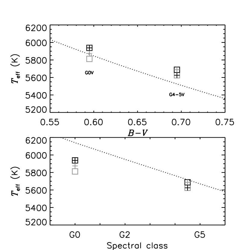
Figure 14: Same as Fig. 13, but for the dwarfs.

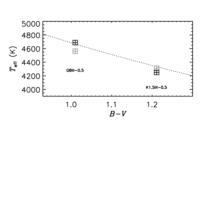
Figure 15: Same as Fig. 15, but for the metal poor stars. Note that BBCR04 only analyzed solar metallicity stars, so we only show a comparison to the $T_{\rm eff}$ calibration of RM05.

Table 1: List of stars selected from B85 catalog for SED fitting. Spectral types are from the sources cited in Section 2, $V$ values are from BSC5, and the [${{\rm A}\over{\rm H}}$] values are from Cayrel et al. (2001).

	Spectral		Mean or median	Num	Num
Object	type	$V$	[${{\rm A}\over{\rm H}}$]	[${{\rm A}\over{\rm H}}$]	spectra
HD50522	G5 III-IV	4.35	0.05	1	1
HD71369	G5 III	3.36	-0.05	2	2
HD34559	G8 III	4.94	-0.10	1	1
HD62345	G8 IIIa	3.57	0.00	1	3
HD100407	G7 III	3.54	-0.04	1	1
HD115659	G8 IIIa	3.00	-0.02	2	1
HD147675	G8 K0III	3.89	-0.05	1	1
HD192947	G8 IIIb	3.57	-0.03	2	1
HD7106	K0.5 IIIb	4.51	-0.04	1	2
HD61935	K0 III	3.93	-0.10	2	2
HD62509	K0 IIIb	1.14	-0.10	7	2
HD123139	K0 IIIb	2.06	0.04	2	1
HD125351	K0 III	4.81	-0.08	2	1
HD177241	G9 IIIb	3.77	0.03	2	1
HD188947	K0 III	3.89	0.05	2	1
HD205512	K0.5 III	4.90	0.05	4	2
HD216228	K0 III	3.52	0.03	3	1
HD219449	K0 III	4.21	-0.08	2	1
HD62044	K1 III	4.28	-0.02	1	1
HD71878	K1 III	3.77	-0.01	1	1
HD206952	K1 III	4.56	0.04	1	1
HD156266	K2 III	4.73	-0.03	1	1
HD161096	K2 III	2.77	0.06	2	2
HD49878	K4 III	4.55	0.05	1	1
HD81817	K3 IIIa	4.29	0.09	1	1
HD211073	K3 III	4.49	-0.07	2	1
HD221673	K4 IIIb	4.98	-0.03	1	1
HD115383	G0 V	5.22	0.08	5	1
HD141004	G0 V	4.43	-0.02	6	1
HD20630	G5 V	4.83	0.01	3	1
HD117176	G4 V	4.98	-.08	4	1
HD138905	G8.5 III	3.91	-0.41	2	1
HD222107	G8 III-IV	3.82	-0.49	2	2
HD124897	K1.5 IIIFe-0.5	-0.04	-0.54	17	3

Table 2: Series 1 models: Closest match models to mean sample spectra and goodness of fit statistics.

	Total SED		Blue	Red
Spectral type	$T_{\rm eff}$ ($\sigma$)	$\log g$	$T_{\rm eff}$ ($\sigma$)	$T_{\rm eff}$ ($\sigma$)	[${{\rm A}\over{\rm H}}$]
G5 III	$\cdots$	2.5	5312 (0.058)	$\cdots$	0.0
G8 III	5125 (0.039)	2.5	5125 (0.058)	5062 (0.013)	0.0
K0 III	4875 (0.049)	2.0	4875 (0.077)	4812 (0.012)	0.0
K0 III	4938 (0.046)	2.0	4938 (0.069)	4875 (0.016)	0.0
K0 III	4812 (0.059)	2.0	4812 (0.093)	4750 (0.016)	0.0
K1 III	4688 (0.079)	2.5	4688 (0.125)	4625 (0.014)	0.0
K2 III	4562 (0.062)	2.0	4562 (0.098)	4500 (0.017)	0.0
K3-4 III	4250 (0.109)	2.0	4250 (0.169)	4188 (0.041)	0.0
G0 V	5938 (0.039)	4.5	5938 (0.059)	5812 (0.014)	0.0
G4-5 V	5688 (0.049)	4.5	5688 (0.075)	5625 (0.021)	0.0
G8 III	4688 (0.063)	2.5	4688 (0.094)	4562 (0.013)	-0.5
K1.5 III	4250 (0.095)	2.0	4250 (0.147)	4312. (0.026)	-0.5

Table 3: Series 2 models: Same as Table 2.

	Total SED		Blue	Red
Spectral type	$T_{\rm eff}$ ($\sigma$)	$\log g$	$T_{\rm eff}$ ($\sigma$)	$T_{\rm eff}$ ($\sigma$)	[${{\rm A}\over{\rm H}}$]
G5 III	$\cdots$	2.5	5312 (0.065)	$\cdots$	0.0
G8 III	5125 (0.037)	2.0	5125 (0.057)	5062 (0.012)	0.0
K0 III	4812 (0.051)	2.0	4812 (0.082)	4812 (0.012)	0.0
K0 III	4875 (0.046)	2.0	4875 (0.074)	4875 (0.014)	0.0
K0 III	4750 (0.057)	2.0	4750 (0.090)	4750 (0.018)	0.0
K1 III	4625 (0.074)	2.5	4625 (0.121)	4625 (0.015)	0.0
K2 III	4500 (0.059)	2.0	4500 (0.095)	4500 (0.018)	0.0
K3-4 III	4250 (0.101)	1.5	4250 (0.155)	4188 (0.036)	0.0
G0 V	5938 (0.048)	4.5	5938 (0.076)	5875 (0.012)	0.0
G4-5 V	5625 (0.060)	4.5	5625 (0.094)	5688 (0.022)	0.0
G8 III	4688 (0.058)	2.5	4688 (0.086)	4562 (0.013)	-0.5
K1.5 III	4250 (0.096)	2.0	4250 (0.149)	4312 (0.027)	-0.5

Table 4: Comparison with empirical $T_{\rm eff}$ calibrations of RM05 and BBCR04.

		Series 1		Series 2
Spectral type	B-V    ($\sigma$)	Blue	Red	Blue	Red	RM05	BBCR04	B10
G5 III	0.882 (0.019)	5312	$\cdots$	5312	$\cdots$	5137	5410	$\cdots$
G8 III	0.930 (0.004)	5125	5062	5125	5062	4964	5123	$\cdots$
K0 III	1.043 (0.002)	4875	4812	4812	4812	4721	4870	$\cdots$
K0 III	1.018 (0.011)	4938	4875	4875	4875	4781	4870	$\cdots$
K0 III	1.080 (0.000)	4812	4750	4750	4750	4650	4870	$\cdots$
K1 III	1.115 (0.003)	4688	4625	4625	4625	4592	4710	4737
K2 III	1.160 (0.006)	4562	4500	4500	4500	4531	4550	4562
K3-4 III	1.408 (0.014)	4250	4188	4250	4188	4118	4243	4134
G0 V	0.595 (0.004)	5983	5812	5938	5875	5864	6140	$\cdots$
G4-5 V	0.695 (0.010)	5688	5625	5625	5688	5519	5670	$\cdots$
G8 III-0.5	1.010 (0.000)	4688	4562	4688	4562	4684	$\cdots$	$\cdots$
K1.5 III-0.5b	1.211 (0.009)	4250	4312	4250	4312	4332	$\cdots$	4386

References

- Abt (2008) Abt, H.A., 2008, ApJS,176,216
- Abt (1981) Abt, H.A., 1981, ApJS,45,437
- Adams et al. (1935) Adams, W.S., Joy, A.H., Humason, M.L. & Brayton, A.M., 1935, ApJ,81,187
- Alonso et al. (1999) Alonso, A., Arribas, S., Martinez-Roger, C., 1999, A&A, 139, 335
- Asplund et al. (2004) Asplund, M., Grevesse, N., Sauval, A.J., Allende Prieto, C. & Kiselman, D., 2004, A&A, 417, 751
- Baines et al. (2010) Baines, E.K., Dollinger, M.P., Cusano, F., Guenther, E.W., Hatzes, A.P., McAlister, H.A., ten Brummelaar, T.A., Turner, N.H., Sturmann, J., Sturmann, L., Goldfinger, P.J., Farrington, C.D., & Ridgway, S.T., 2010, ApJ, 710, 1365 (B10)
- Bertone et al. (2004) Bertone, E., Buzzoni, A., Chavez, M. & Rodriguez-Merino, L.H., 2004, ApJ, 128, 829 (BBCR04)
- Burnashev (1985) Burnashev V.I., 1985, Abastumanskaya Astrofiz. Obs. Bull. 59, 83 (B85)
- Cayrel et al. (2001) Cayrel de Strobel, G., Soubiran C., Ralite N., 2001, A&A, 373, 159
- Foy (1978) Foy, R., 1978 A&A, 67, 311
- Gray (1982) Gray, D.F., 1982, ApJ, 262, 682
- Gray et al. (2006) Gray, R.O., Corbally, C.J., Garrison, R.F., McFadden, M.T., Bubar, E.J., McGahee, C.E., O’Donoghue, A.A. & Knox, E.R., 2006, AJ,132,161
- Gray et al. (2003) Gray, R.O., Corbally, C.J., Garrison, R.F., McFadden, M.T. & Robinson, P.E., 2003, AJ,126,2048
- Grevesse et al. (1992) Grevesse, N., Noels, A., Sauval, A.J., 1992, In ESA, Proceedings of the First SOHO Workshop, p. 305
- Gunn & Stryker (1983) Gunn, J.E. & Stryker, L.L., 1983, ApJS, 52, 121
- Gustafsson et al. (1974) Gustafsson, B., Kjaergaard, P., Andersen, S., 1974, A&A, 34, 99
- Harlan (1974) Harlan, E.A., 1974, AJ,79,682
- Hauschildt et al. (1999a) Hauschildt, P., Allard, F., & Baron, E., 1999, ApJ, 512, 377
- Hauschildt et al. (1999b) Hauschildt, P.H., Allard, F., Ferguson, J., Baron, E. & Alexander, D.R., 1999, ApJ, 525, 871
- Hoffleit & Warren (1991) Hoffleit, E.D., Warren, Jr. W.H., “The Bright Star Catalogue, 5th Revised Ed., 1991, Astronomical Data Center, NSSDC/ADC (BSC5)
- Houk & Cowley (1975) Houk N. & Cowley A.P., 1975, “Michigan Catalogue of two dimentional spectral types for the HD stars, Vol. 1”, Ann Arbor, Univ. of Michigan
- Jacoby et al. (1984) Jacoby, G.H., Hunter, D.A. & Christian, C.A., 1984, ApJS, 56, 257
- Keenen & Barnbaum (1999) Keenan, P.C. & Barnbaum, C., 1999, ApJ, 518, 859
- Keenan & McNeil (1989) Keenan,P.C. & McNeil R.C., 1989, ApJS, 71, 245
- Keenan & Newsom (2000) Keenan,P.C. & Newsom, G.H., 2000, The Revised Catalog of MK Spectra Types for the Cooler Stars, www.astronomy.ohio-state.edu/MKCool/
- Kurucz (1992a) Kurucz, R.L., 1992, Rev. Mex. Astron. Astrofis., 23, 181
- Kurucz & Peytremann (1975) Kurucz, R.L. & Peytremann, E., 1975, SAO Special Rep. 362, pt. 1
- Kurucz et al. (1987) Kurucz, R.L., van Dishoeck, E.F. & Tarafdar, S.P., 1987, ApJ, 322, 992
- Mermilliod (1991) Mermilliod, J.C., 1991, “Catalogue of Homogeneous Means in the UBV System”, Lausanne
- Neckel & Labs (1984) Neckel, H. & Labs, D., 1984, Sol. Phys., 90, 205
- Peterson et al. (1993) Peterson, R.C., Dalle Ore, C.M., Kurucz, R.L., 1993, ApJ, 404, 333
- Pinsonneault & Delahaye (2009) Pinsonneault, M.H. & Delahaye, F., 2009, ApJ, 704, 1174