Nuclei as near BPS-Skyrmions

Abstract

We study a generalization of the Skyrme model with the inclusion of a sixth-order term and a generalized mass term. We first analyze the model in a regime where the nonlinear $\sigma$ and Skyrme terms are switched to zero which leads to well-behaved analytical BPS-type solutions. Adding contributions from the rotational energy, we reproduce the mass of the most abundant isotopes to rather good accuracy. These BPS-type solutions are then used to compute the contributions from the nonlinear sigma and Skyrme terms when these are switched on. We then adjust the four parameters of the model using two different procedures and find that the additional terms only represent small perturbations to the system. We finally calculate the binding energy per nucleon and compare our results with the experimental values.

I Introduction

The Skyrme model Skyrme is nowadays one of the strongest candidates for a description of the low-energy regime of QCD. Developed in the beginning of the 60’s by T.H.R. Skyrme, it consists of a nonlinear theory of mesons where its main feature is the presence of topological solitons as solutions. Each of these solutions is associated with a conserved topological charge, the winding number, which Skyrme interpreted as the baryon number, thus leading him to state that the solitons are baryons emerging from a meson field. The $\frac{1}{N_{C}}$ expansion of QCD introduced by t’Hooft thooft in the mid-70’s and the later connection from Witten Witten with the model developed by Skyrme brought some support to this interpretation.

Since its original formulation, the Skyrme model has been able to predict the properties of the nucleon within a precision of 30%. Several modifications to the model have been considered to improve these predictions, from the generalization of the mass term Marleau1 ; KPZ ; Marleau2 to the explicit addition of vector mesons Sutcliffe ; Adkins2 , aside form higher order terms in derivatives of the pion field Marleau1 . Unfortunately, the analysis of these models has been hampered by their nonlinear nature and the absence of analytical solutions. Indeed, all the solutions rely on numerical computation at some point whether one uses the rational map ansatz Houghton , which turns out to be a rather good approximation of the angular dependance, or a full fledge numerical algorithm like simulated annealing Marleau3 ; Houghton2 to find an exact solution of the energy functional. Clearly, even a prototype model with analytical solutions would allow to go deeper in the investigation of the properties and perhaps identify novel features of the Skyrmions.

In a recent study, Adam, Sanchez-Guillen and Wereszczynski (ASW) Adam obtained an analytical solution by considering a model consisting only of a term of order six in derivatives and a potential which correspond to the customary mass term for pions in the Skyrme model Adkins . Their calculations lead to a compacton-type solution with size growing as $n^{\frac{1}{3}}$, with $n$ is the winding number, a result in general agreement with experimental observations. Another important remark on their study is that their solutions are of BPS-type, i.e. they saturate a Bogomolny’s bound. Even though physical nuclei do not saturate such a bound, the small value of the binding energy may be one of the motivation for solution of this type. Let us also mention that recently Sutcliffe Sutcliffe2 found that BPS-type Skyrmions also emerge from models when a large number of vector mesons are added to the Skyrme model. However, the analysis of ASW neglects rotational or isorotational energies of nuclei and perhaps the oddest feature of the model is that it does not contain any of the terms that Skyrme originally introduced in his model, the nonlinear sigma and so-called Skyrme terms which are of order 2 and 4 in derivatives respectively. Being a effective theory of QCD, there is nevertheless no reason to omit such contributions. In their work ASW further suggest that their analytical solutions found could be used to compute the contributions from the terms of the original Skyrme lagrangian assuming they are small and do not affect significantly the overall solutions. Unfortunately the nature of the solution leads to singularities in the computation of the energies related to the nonlinear sigma and Skyrme terms.

In this work, we find analytical BPS-type solutions for a Lagrangian similar to the one in Adam which allows to consider contributions from the original Skyrme Lagrangian as small perturbations. The analysis also includes contributions for (iso)rotational energies providing a more realistic description of nuclei. The paper is divided as follows: In section II, we introduce the general form of this generalized Skyrme model and find expressions for the static energies. Next, we quantify semiclassically the zero modes of the Skyrmions, which will allow to compute rotational contributions to the total energy coming from the spin as well as the isospin of the nuclei. In section IV, we choose an adequate potential (or mass term) and switch off the nonlinear sigma and Skyrme terms. We then find a simple analytical form of the BPS-type solutions for the remaining Lagrangian. It turns out that all the properties of the nuclei can be calculated analytically. In section V, we use the solution to compute the properties of the full Lagrangian. Fitting the different parameters of the model with nuclear mass data Nucltable we verify that the contributions from the nonlinear sigma and Skyrme terms remain small and that the analytical solution is a good approximation.

II Lagrangian of the Skyrme model

The model proposed by ASW is based on the Lagrangian density

$$\mathcal{L}=\mathcal{L}_{6}-\mu^{2}V=-\frac{3}{2}\frac{\lambda^{2}}{16^{2}}\text{Tr}\left(\left[L_{\mu},L_{\nu}\right]\left[L^{\nu},L^{\lambda}\right]\left[L_{\lambda},L_{\mu}\right]\right)-\frac{1}{2}\mu^{2}\text{Tr}\left[1-U\right].$$ (1)

where $U=\phi_{0}+i\tau_{i}\phi_{i}$ is the $SU(2)$ matrix representing the meson fields and $L_{\mu}=U^{\dagger}\partial_{\mu}U$ is the left-handed current. The model leads to BPS-type solitons. The constants $\lambda$ and $\mu$ are the only free parameters of the model with units MeV^-1 and MeV² respectively. Using scaling arguments, one can show that the term of order 6 in field derivatives, $\mathcal{L}_{6},$ prevents the soliton from shrinking to zero size while the second term, often called the mass term, stabilize the solution against arbitrary expansion.

On the other hand, the original Skyrme model consists of the two completely different terms

$$\mathcal{L}=\mathcal{L}_{nl\sigma}+\mathcal{L}_{Sk}$$ (2)

with

$$\mathcal{L}_{nl\sigma}=\alpha\text{Tr}\left[L_{\mu}L^{\mu}\right],\qquad\mathcal{L}_{Sk}=\beta\text{Tr}\left(\left[L_{\mu},L_{\nu}\right]^{2}\right)$$ (3)

the nonlinear sigma and so-called Skyrme terms which are of order 2 and 4 in derivatives respectively. Here $\left[\alpha\right]=\text{MeV}^{2}$ and $\beta$ is a dimensionless constant.

We shall consider here a model containing the four terms i.e. an extension of the Skyrme model with a sixth order term in derivatives and generalized mass term. The Lagrangian density reads

$$\mathcal{L}=-\mu^{2}V(U)-\alpha\text{Tr}\left[L_{\mu}L^{\mu}\right]+\beta\text{Tr}\left(\left[L_{\mu},L_{\nu}\right]^{2}\right)-\frac{3}{2}\frac{\lambda^{2}}{16^{2}}\text{Tr}\left(\left[L_{\mu},L_{\nu}\right]\left[L^{\nu},L^{\lambda}\right]\left[L_{\lambda},L_{\mu}\right]\right)$$ (4)

We are interested in the regime where $\alpha$ and $\beta$ are small so that $\mathcal{L}_{nl\sigma}$ and $\mathcal{L}_{Sk}$ can be considered as small perturbations to (1). Usually, the potential $V(U)$ is chosen such that it reproduces the mass term for pions when small fluctuations of the fields are considered

$$U=e^{2i\tau_{i}\frac{\pi_{i}}{F_{\pi}}}\sim 1+2i\tau_{i}\frac{\pi_{i}}{F_{\pi}}.$$ (5)

where $F_{\pi}=4\sqrt{\alpha}$ is the pion decay constant. Since $U$ is an $SU\left(2\right)$ matrix, the meson fields obey the condition

$$\phi_{0}^{2}+\phi_{i}^{2}=1$$ (6)

to limit the degrees of freedom to three. The boundary condition

$$U\left(r\rightarrow\infty\right)=\mathcal{I}_{2\times 2}$$ (7)

with $\mathcal{I}_{2\times 2}$ the two-dimensional unit matrix, ensures that each solution for the Skyrme field falls into a topological sector characterized by a conserved topological charge

$$B=-\frac{\epsilon^{ijk}}{48\pi^{2}}\int d^{3}x\text{Tr}\left(L_{i}\left[L_{j},L_{k}\right]\right).$$ (8)

The static energy can then be calculated using

$$E_{stat}=-\int d^{3}x\mathcal{L}_{stat}.$$ (9)

We may conveniently write a general solution as

$$U=e^{i\mathbf{n}\cdot\mathbf{\tau}F}=\cos F+i\mathbf{n}\cdot\mathbf{\tau}\sin F$$ (10)

where $\mathbf{\hat{n}}$ is the unit vector

$$\mathbf{\hat{n}}=\left(\sin\Theta\cos\Phi,\sin\Theta\sin\Phi,\cos\Theta\right)$$

or

$$\phi_{a}=\left(\cos F,\sin F\sin\Theta\cos\Phi,\sin F\sin\Theta\sin\Phi,\sin F\cos\Theta\right).$$

Following ASW Adam , we consider solutions of the form that saturates the Bogomolny’s bound for (1)

$$F=F(r),\qquad\Theta=\theta,\qquad\Phi=n\phi$$ (11)

where $n$ is an integer. The static energy (4) becomes

$$E_{stat} =-\int d^{3}x\mathcal{L}_{stat}=4\pi\int r^{2}dr\left(\mu^{2}V+\frac{9\lambda^{2}}{16}n^{2}F^{\prime}{}^{2}\frac{\sin^{4}F}{r^{4}}\right.$$ (12)

$$+\left.2\alpha\left[F^{\prime 2}+\left(n^{2}+1\right)\frac{\sin^{2}F}{r^{2}}\right]+16\beta\frac{\sin^{2}F}{r^{2}}\left[\left(n^{2}+1\right)F^{\prime 2}+n^{2}\frac{\sin^{2}F}{r^{2}}\right]\right)$$

where $F^{\prime}=\partial F/\partial r$ and the topological charge is simply $B=n$.

In order to represent physical nuclei, we have to quantize the solitons using a semiclassical method described in the next section. Using the appropriate spin and isospin numbers, we will then be able to calculate the total energy for each nuclei.

III Quantization

Because the topological solitons occupy a spatial volume that is nonzero, usual quantization procedures are no longer available. We therefore have to use a semiclassical quantization method by adding an explicit time dependence to the zero modes of the Skyrmion. Performing time-dependent (iso)rotations on the Skyrme field by $SU(2)$ matrix $A(t)$ and $B(t)$ yield

$$\tilde{U}\left(\mathbf{r},t\right)=A(t)U\left(R(B(t))\mathbf{r}\right)A(t)$$ (13)

where $R_{ij}(B(t))=\frac{1}{2}\text{Tr}\left[\tau_{i}B\tau_{j}B^{\dagger}\right]$ is the associated $SO(3)$ rotation matrix. Upon insertion of this ansatz in the time-dependent part of (4), we write the rotational lagrangian as

$$\mathcal{L}_{rot}=\frac{1}{2}a_{i}U_{ij}a_{j}-a_{i}W_{ij}b_{j}+\frac{1}{2}b_{i}V_{ij}b_{j}$$ (14)

with $U_{ij}$, $V_{ij}$ and $W_{ij}$ the inertia tensors

$$U_{ij} =-\int\text{d}^{3}x\biggl{\{}2\alpha\text{Tr}\left(T_{i}T_{j}\right)+4\beta\text{Tr}\left(\left[L_{k},T_{i}\right]\left[L_{k},T_{j}\right]\right)\biggr{.}$$

$$\biggl{.}+\frac{9\lambda^{2}}{16^{2}}\text{Tr}\left(\left[T_{i},L_{k}\right]\left[L_{k},L_{n}\right]\left[L_{n},T_{j}\right]\right)\biggr{\}},$$ (15)

$$V_{ij} =-\epsilon_{ikl}\epsilon_{jmn}\int\text{d}^{3}xx_{k}x_{m}\biggl{\{}2\alpha\text{Tr}\left(L_{l}L_{n}\right)+4\beta\text{Tr}\left(\left[L_{p},L_{l}\right]\left[L_{p},L_{n}\right]\right)\biggr{.}$$

$$\biggl{.}+\frac{9\lambda^{2}}{16^{2}}\text{Tr}\left(\left[L_{l},L_{p}\right]\left[L_{p},L_{q}\right]\left[L_{q},L_{n}\right]\right)\biggr{\}},$$ (16)

$$W_{ij} =\epsilon_{jkl}\int\text{d}^{3}xx_{k}\biggl{\{}2\alpha\text{Tr}\left(T_{i}L_{l}\right)+4\beta\text{Tr}\left(\left[L_{p},T_{j}\right]\left[L_{p},L_{n}\right]\right)\biggr{.}$$

$$\biggr{.}+\frac{9\lambda^{2}}{16^{2}}\text{Tr}\left(\left[T_{i},L_{m}\right]\left[L_{m},L_{n}\right]\left[L_{n},L_{l}\right]\right)\biggr{\}}$$ (17)

and $T_{i}=iU^{\dagger}\left[\frac{\tau_{i}}{2},U\right]$. Assuming a solution of the form (10), the inertia tensors becomes all diagonal and furthermore, one can show that $U_{11}=U_{22}\neq U_{33}$ with similar identities for the $V_{ij}$ and $W_{ij}$ tensors. Finally the general expressions for the moments of inertia coming from each pieces of the Lagrangian read

$$U_{11} =\frac{4\pi}{3}\int r^{2}dr\sin^{2}F\left(8\alpha+16\beta\left[4F^{\prime 2}+\left(3n^{2}+1\right)\frac{\sin^{2}F}{r^{2}}\right]+\frac{9\lambda^{2}}{4}\frac{\left(3n^{2}+1\right)}{4}F^{\prime 2}\frac{\sin^{2}F}{r^{2}}\right),$$ (18)

$$V_{11} =\frac{4\pi}{3}\int r^{2}dr\sin^{2}F\left(2\left(n^{2}+3\right)\alpha+16\beta\left[\left(n^{2}+3\right)F^{\prime 2}+4n^{2}\frac{\sin^{2}F}{r^{2}}\right]+\frac{9\lambda^{2}}{4}n^{2}F^{\prime 2}\frac{\sin^{2}F}{r^{2}}\right),$$ (19)

and the general expression for $U_{33}$ can be obtained by setting $n=1$ in the integrand of (18). It turns out that expressions (15)-(17) leads to $W_{11}=W_{22}=0$ for $\left|n\right|\geq 2$ and $n^{2}U_{33}=nW_{33}=V_{33}$. Otherwise, for $\left|n\right|=1$ we have spherical symmetry and,

$$W_{11}=\frac{4\pi}{3}\int r^{2}dr\sin^{2}F\left(8\alpha+16\beta\left(4\frac{\sin^{2}F}{r^{2}}+4F^{\prime}\right)+\frac{9\lambda^{2}}{4}F^{\prime 2}\frac{\sin^{2}F}{r^{2}}\right).$$ (20)

Following Houghton and Magee Houghton2 , we now write the rotational hamiltonian as

$$H_{rot}=\frac{1}{2}\left[\frac{\left(L_{1}+W_{11}\frac{K_{1}}{U_{11}}\right)^{2}}{V_{11}-\frac{W_{11}^{2}}{U_{11}}}+\frac{\left(L_{2}+W_{22}\frac{K_{2}}{U_{22}}\right)^{2}}{V_{22}-\frac{W_{22}^{2}}{U_{22}}}+\frac{\left(L_{3}+W_{33}\frac{K_{3}}{U_{33}}\right)^{2}}{V_{33}-\frac{W_{33}^{2}}{U_{33}}}+\frac{K_{1}^{2}}{U_{11}}+\frac{K_{2}^{2}}{U_{22}}+\frac{K_{3}^{2}}{U_{33}}\right]$$ (21)

with ($K_{i}$) $L_{i}$ the body-fixed (iso)rotation momentum canonically conjugate to $a_{i}$ and $b_{i}$ respectively. The expression for the rotational energy of the nucleon has been obtained in Houghton2 and reads, for a spherical symmetry

$$E_{rot}^{N}=\frac{3}{8U_{11}}.$$ (22)

For the deuteron, the rotational energy has been calculated assuming an axial symmetric solution Marleau4

$$E_{rot}^{D}=\frac{1}{2V_{11}}+\frac{1}{2V_{22}}$$ (23)

which reduces to

$$E_{rot}^{D}=\frac{1}{V_{11}}$$ (24)

for the axial ansatz (10). It is easy to calculate the rotational energies for nuclei with winding number $\left|n\right|\geq 3$. The axial symmetry of the solution imposes the constraint $L_{3}+nK_{3}=0$ which is simply the statement that a spatial rotation by an angle $\theta$ about the axis of symmetry can compensated by an isorotation of $-n\theta$ about the $\tau_{3}$ axis. It also implies that$\ n^{2}U_{33}=nW_{33}=V_{33}$. Recalling that $W_{11}=W_{22}=0$ for these values of $n$, the rotational hamiltonian reduces to

$$H_{rot}=\frac{1}{2}\left[\frac{\mathbf{L}^{2}}{V_{11}}+\frac{\mathbf{K}^{2}}{U_{11}}+\left(\frac{1}{U_{33}}-\frac{1}{U_{11}}-\frac{n^{2}}{V_{11}}\right)K_{3}^{2}\right]$$ (25)

These momenta are related to the usual space-fixed isospin ($\mathbf{I}$) and spin ($\mathbf{J}$) by the orthogonal transformations

$$I_{i}=-R(A_{1})_{ij}K_{j},$$ (26)

$$J_{i}=-R(A_{2})_{ij}^{\text{T}}L_{j}.$$ (27)

According to (26) and (27), we see that the Casimir invariants satisfy $\mathbf{K}^{2}=\mathbf{I}^{2}=I(I+1)$ and $\mathbf{L}^{2}=\mathbf{J}^{2}=J(J+1)$ so the rotational hamiltonian is given by

$$H_{rot}=\frac{1}{2}\left[\frac{J(J+1)}{V_{11}}+\frac{I(I+1)}{U_{11}}+\left(\frac{1}{U_{33}}-\frac{1}{U_{11}}-\frac{n^{2}}{V_{11}}\right)K_{3}^{2}\right].$$ (28)

IV BPS-type solutions

Let’s consider a model similar to Adam composed of the term of order six in derivatives plus a potential by setting $\alpha$, $\beta=0$

$$\mathcal{L}=-\frac{3}{2}\frac{\lambda^{2}}{16^{2}}\text{Tr}\left(\left[L_{\mu},L_{\nu}\right]\left[L^{\nu},L^{\lambda}\right]\left[L_{\lambda},L_{\mu}\right]\right)-\mu^{2}V(U).$$ (29)

Using the results of section II, the static energy is

$$E_{stat}=4\pi\int dr\left(\frac{9\lambda^{2}n^{2}}{4}\frac{\sin^{4}F}{4r^{2}}F^{\prime 2}+\mu^{2}V(U)\right).$$ (30)

The minimization of the static energy of the soliton, leads to the differential equation for $F$

$$\frac{9\lambda^{2}n^{2}}{4}\frac{\sin^{2}F}{2r^{2}}\partial_{r}\left(\frac{\sin^{2}F}{r^{2}}F^{\prime}\right)-\mu^{2}V_{F}=0.$$ (31)

A change of variable $z=\frac{2\sqrt{2}\mu r^{3}}{9n\lambda}$ allows to rewrite (31) in a simple form

$$\sin^{2}F\partial_{z}\left[\sin^{2}F\left(\partial_{z}F\right)\right]-\mu^{2}\frac{\partial V}{\partial F}=0.$$ (32)

This last equation can be integrated

$$\frac{1}{2}\sin^{4}F\left(F_{z}\right)^{2}=V$$ (33)

and inserting the expression for $z$, provide an expression which amounts to a statement of equipartition of the energy, i.e. the term of order 6 in derivatives and the potential contribute equally to the total energy. ASW has shown that a solution of (33) saturates the Bogomolny’s bound Adam . From (33) we obtain the following useful relation between the function $F$ and the potential

$$\int dF\frac{\sin^{2}F}{\sqrt{2V}}=\pm\left(z-z_{0}\right)$$ (34)

with $z_{0}$ an integration constant.

Now comes the time to choose a specific potential. The choice for mass term of the Skyrme is not unique and indeed has been the object of several discussions Adkins ; Marleau1 ; KPZ . The usual mass term $V=1-\cos F$ was considered in Adam . Solving (34) for $F$

$$F(r)=\left\{\begin{tabular}[c]{lll}$2\arccos\left(\nu r^{3}\right)$&$\qquad\text{for}$&$r\in\left[0,\nu^{-\frac{1}{3}}\right]$\\ $0$&$\qquad\text{for}$&$r\geq\nu^{-\frac{1}{3}}$\end{tabular}\text{ }\right.$$ (35)

where $\nu=\frac{\mu}{18n\lambda}$ is a constant depending on the parameters $\lambda$, $\mu$ and $n$. Note that $F^{\prime}$ diverges as $\ r\rightarrow\nu^{-\frac{1}{3}}.$ Since this solution saturates the Bogomolny’s bound, the static energy is proportional to the baryon number $B=n$ .

A question arises as how would the nonlinear $\sigma$ and Skyrme term affect the energy of such Skyrmions. Switching them on slowly by moving $\alpha$ and $\beta$ away from zero could give an estimate of their contributions. Unfortunately, it turns out that simply substituting the solution (35) in the expression for energy associated with the full Lagrangian leads to divergences. So, however small the parameters $\alpha$ and $\beta$ are, these BPS solutions cannot be considered as appropriate approximations of the solutions for (4).

Yet it could be interesting to analyze the full Lagrangian (4) in a regime close to a BPS Skyrmion. For this purpose, we propose to write the potential in the form of the generalized mass term introduced by Marleau1

$$V =-\sum_{k=1}^{\infty}C_{k}\text{Tr}\left[U^{k}+U^{\dagger k}-2\right]$$

$$=-4\pi\sum_{k=1}^{\infty}\int r^{2}dr8C_{k}\sin^{2}\left(\frac{k\xi}{2}\right).$$ (36)

The main motivation for this choice is that the potential can be written in a simple form in terms of pion fields. Furthermore this particular framework insures that one recovers the chiral symmetry breaking pion mass term $-\frac{1}{2}m_{\pi}^{2}\mathbf{\pi}\cdot\mathbf{\pi}$  in the limit of small pion field fluctuations provided

$$\sum_{k=1}^{\infty}k^{2}C_{k}=-\frac{m_{\pi}^{2}F_{\pi}^{2}}{16}.$$ (37)

For practical purposes, one requires (i) an expression of the potential that is simple enough to allow the analytical integration of the left-hand side of equation (34), (ii) that the results leads to an invertible function to be able to write the chiral profile $F$ as a function of $r$ and finally (iii) that $F\left(r\right)$ is well behaved. A most convenient choice is

$$V=\sin^{2}\left(\frac{F}{2}\right)\cos^{6}\left(\frac{F}{2}\right).$$ (38)

Expanding the expression (38), the coefficients $C_{k}$ are

$$C_{1}=-\frac{\mu^{2}}{128},\qquad C_{2}=\frac{\mu^{2}}{128},\qquad C_{3}=\frac{\mu^{2}}{128},\qquad C_{4}=\frac{\mu^{2}}{512},\qquad C_{k>4}=0.$$ (39)

Integrating (34) we get the general solution

$$F(r)=2\arccos\left(e^{\pm\nu\left(r^{3}-r_{0}^{3}\right)}\right)$$ (40)

with $\nu=\frac{\mu}{18n\lambda}$. In order that the baryon number corresponds to $\left|B\right|=n,$ one must require that

$$F(\infty)-F(0)=\mp\pi$$

for $B$ positive or negative respectively. Accordingly we choose the boundary conditions $F(0)=0$ and $F(\infty)=\mp\pi$ which sets the integration constant $r_{0}$ to zero and allows to write

$$F(r)=\mp 2\left|\arccos\left(e^{-\nu r^{3}}\right)\right|$$ (41)

where we use the absolute value to dispose of the sign ambiguity of the arccos function. Note that here contrary to Adam we do not get a compacton type solution but a well behaved function with a continuous first derivative. All calculations regarding energy can be performed analytically, i.e. static energy and the moments. For example, the baryon density is given by the radial function

$$B(r)=\frac{2\mu}{3\pi^{2}\lambda}e^{-\frac{\mu r^{3}}{6n\lambda}}\left(1-e^{-\frac{\mu r^{3}}{9n\lambda}}\right)$$

which upon integration leads to baryon number $B=n.$ Experimentally the size of the nucleus is known to behave as

$$R=R_{0}B^{\frac{1}{3}}=\left(1.25\text{ fm}\right)B^{\frac{1}{3}}$$

where $R_{0}=1.25$ fm. It is interesting to note that the baryon number distribution is zero at $r=0$ but has maximum value $\frac{\sqrt{3}\mu}{8\pi^{2}\lambda}$ independent of $n$ which is positioned at

$$r_{\max}=\left(\frac{9\lambda}{\mu}\ln\left(\frac{4}{3}\right)\right)^{\frac{1}{3}}B^{\frac{1}{3}}$$ (42)

where $r_{\max}$ here is in units of MeV^-1. Accordingly the size of the nucleus $r_{\max}$  is proportional to $B^{\frac{1}{3}}$ with $R_{0}$ depending only on the ratio $\lambda/\mu$. Similarly expressions can be obtained for energy and moment of inertia density. Using (40), they yield

$$E =2n\pi\mu\lambda$$

$$V_{11} =n^{2}U_{33}=\frac{4n^{2}}{\left(3n^{2}+1\right)}U_{11}=2\pi\left(\frac{\lambda n}{3\mu}\right)^{\frac{5}{3}}\mu^{2}\Gamma\left(\frac{2}{3}\right)\left(16\cdot 3^{\frac{1}{3}}-9\cdot 2^{\frac{2}{3}}\right)$$ (43)

where $\Gamma\left(x\right)$ is the gamma function. Combining these results in (28)

$$H_{rot}=\frac{1}{2U_{11}}\left[J(J+1)\frac{\left(3n^{2}+1\right)}{4n^{2}}+I(I+1)-K_{3}^{2}\right].$$ (44)

Note that this last result only hold for $\alpha=\beta=0$ and the solution (40). The last term is either zero or negative. Depending on the dimension of the spin and isospin representation, the diagonalization of this hamiltonian will lead to a number of eigenstates. We are interested in the lowest eigenvalue of $H_{rot}$ which points towards the eigenstate $\left|i,i_{3},k_{3}\right\rangle\left|j,j_{3},l_{3}\right\rangle$ with the largest possible eigenvalue $k_{3}.$ Since $\mathbf{K}^{2}=\mathbf{I}^{2}$ and $\mathbf{L}^{2}=\mathbf{J}^{2},$ the state with highest weight is characterized by $k_{3}=I$ and $l_{3}=j$ and since since nuclei are build of $B$ fermions $j\leq B/2.$ On the other hand the axial symmetry of the solutions implies that $k_{3}=-l_{3}/n.$ We recall that these solutions are approximations. Then for even $B$ nuclei, the integer part of $\left|l_{3}/n\right|$ is

$$0\leq\left|k_{3}\right|=\left[\left|\frac{l_{3}}{n}\right|\right]\leq\left[\left|\frac{j}{n}\right|\right]\leq\left[\left|\frac{B}{2n}\right|\right]=0$$

so it leads to $\left|k_{3}\right|=0$. Similarly for half-integer spin nuclei,

$$\frac{1}{2}\leq\left|k_{3}\right|\leq\left|\frac{j}{n}\right|\leq\left|\frac{B}{2n}\right|=\frac{1}{2}$$

So we shall assume for simplicity

$$\kappa=\max(\left|k_{3}\right|)=\left\{\begin{tabular}[c]{l}$0\qquad$for $B=$ even\\ $\frac{1}{2}\qquad$for $B=$ odd\end{tabular}\ \right.$$

The rotational energy is given by

$$E_{rot}=\frac{1}{2U_{11}}\left[j(j+1)\frac{\left(3n^{2}+1\right)}{4n^{2}}+i(i+1)-\kappa^{2}\right].$$ (45)

It remains to fix the values of the parameters $\lambda$ and $\mu$. In order to do so, we choose as input parameters the experimental mass of the nucleon and for simplicity, a nucleus $\ X$ with zero (iso)rotational energy (i.e. a nucleus with zero spin and isospin). The total energy of these two states are

$$E_{N} =\left.\left(E+\frac{3}{8U_{11}}\right)\right|_{n=1}$$

$$=2\pi\mu\lambda+\frac{1}{\mu^{2}}\left(\frac{3\mu}{\lambda}\right)^{\frac{5}{3}}\frac{3}{16\pi\Gamma\left(\frac{2}{3}\right)\left(16\cdot 3^{\frac{1}{3}}-9\cdot 2^{\frac{2}{3}}\right)}$$ (46)

$$E_{X} =\left.E\right|_{n=B}=2B\pi\mu\lambda$$ (47)

Solving for $\lambda$ and $\mu$ we get

$$\lambda =\frac{3\cdot 3^{\frac{1}{4}}}{\left(E_{X}\right)^{\frac{1}{4}}\sqrt{\pi}\left(\left(E_{X}-nE_{N}\right)\left(9\cdot 2^{\frac{2}{3}}-16\cdot 3^{\frac{1}{3}}\right)\Gamma\left(\frac{5}{3}\right)\right)^{\frac{3}{4}}}$$

$$\mu =\frac{\left(E_{X}\right)^{\frac{5}{4}}\left(\left(E_{X}-nE_{N}\right)\left(9\cdot 2^{\frac{2}{3}}-16\cdot 3^{\frac{1}{3}}\right)\Gamma\left(\frac{5}{3}\right)\right)^{\frac{3}{4}}}{24\cdot 3^{\frac{1}{4}}\sqrt{\pi}}$$ (48)

As an example, we choose the nucleus $X$ to be the helium-4, the first doubly magic number nucleus. The mass of the helium-4 nucleus has no (iso)rotational parts since it has zero spin and isospin. Setting the mass of the nucleon as the average mass of the proton and neutron i.e. $E_{N}=938.919$ MeV and the mass of the helium nucleus to $E_{He}=3727.38$ MeV, we obtain the numerical value $\lambda=0.00491505$ MeV^-1 and $\mu=30174.2$ MeV². We shall refer to this set of parameters as Set Ia.

Experimentally the size of the nucleus is known to behave as

$$R=R_{0}B^{\frac{1}{3}}$$

with $R_{0}=1.25$ fm We get a similar behaviour for $r_{\max}$ in (42).

$$r_{\max}=\left(1.4798\text{ fm}\right)B^{\frac{1}{3}}$$ (49)

Combining (48) with (12) and (45), the mass of any nucleus can be expressed as a analytical function of the input parameters $E_{N}$ and $E_{He}$. In general it depends on the baryon number as well as the spin and the isospin of the isotope. The spin of the most abondant isotopes are known. The isospins are not so well known so we resort to the usual assumption that the most abundant isotopes correspond to states with lowest isorotational energy, i.e. states where the isospin $I$ has the lowest value that the conservation of the third component of isospin $I_{3}$ allows. Accordingly,

$$I =\left|I_{3}\right|=\frac{1}{2}\left|\#\text{ of proton }-\#\text{ of neutron}\right|$$

$$=\left|\frac{A}{2}-Z\right|$$ (50)

Table I shows the results for the a few isotopes. The resulting predictions are accurate to $0.3\%$ or better even for heavier nuclei which is rather surprising since the model involves only to two free parameters $\lambda$ and $\mu.$

The computation were repeated using as input parameter $X=$ ¹⁶O and ⁴⁰Ca, two other doubly magic nuclei (also shown in Table I, Set Ib and Set Ic respectively). These set the parameters to $\lambda=0.00449295$ MeV^-1 and $\mu=32977.0$ MeV² and  to $\lambda=0.00426504$ MeV^-1 and $\mu=34717.8$ MeV² respectively. Using these heavier elements as input parameters changes slightly the overall predicting accuracy. Whereas the best overall accuracy is achieved using ¹⁶O parametrization in Set Ib, the lightest isotopes are best described by choosing ⁴He as input (Set Ia). Note that the lightest nuclei have lower moments of inertia and get relatively large rotational contribution to their mass. Consequently their masses are expected to be more sensitive to the parameters affecting rotational energy. Likewise, since the ratio $\lambda/\mu$ decreases for $X=$ ¹⁶O and ⁴⁰Ca, the size of the nucleus also decreases with $R_{0}=1.3943$ fm  and $1.3470$ fm respectively.

Table I: Nuclear masses (MeV)

$$B$$  Nucleus

Set Ia

N+⁴He

Given this unexpected success, one may wonder how switching on the nonlinear $\sigma$ and Skyrme terms can improve or affect these results. Indeed the last results suggest that these contributions need not be be very large. This aspect is analysed in the next section.

V Nonlinear $\sigma$ and Skyrme terms

Let us now consider the full Lagrangian in (4) assuming that the contribution the nonlinear $\sigma$ and Skyrme terms can be set arbitrarily small so that (40) represents a good approximation to the exact solution. Inserting the solution in (12) and in the expression for the various moments of inertia, one get additional contributions proportional to $\alpha$ and $\beta$

$$E_{stat} =2n\pi\mu\lambda+16\pi\alpha\left(\frac{n\lambda}{3\mu}\right)^{\frac{1}{3}}\Gamma\left(\frac{1}{3}\right)\left(\left(2-2^{\frac{2}{3}}\right)\left(n^{2}+1\right)+2\zeta\left(\frac{7}{3}\right)\right)$$

$$+\frac{128\pi\beta}{3}\left(\frac{3\mu}{n\lambda}\right)^{\frac{1}{3}}\Gamma\left(\frac{2}{3}\right)\left(\left(8\left(2\cdot 3^{\frac{1}{3}}-2^{\frac{2}{3}}\right)-7\cdot 2^{\frac{1}{3}}\right)n^{2}+2^{\frac{1}{3}}\right)$$ (51)

and

$$E_{rot}=\frac{1}{2}\left[\frac{j(j+1)}{V_{11}}+\frac{i(i+1)}{U_{11}}+\left(\frac{1}{U_{33}}-\frac{1}{U_{11}}-\frac{n^{2}}{V_{11}}\right)\kappa^{2}\right].$$ (52)

with $\kappa=0$ or $\frac{1}{2}$ for even and odd $B$ respectively and

$$U_{11} =64\pi\alpha\left(\frac{n\lambda}{\mu}\right)+\frac{512\pi\beta}{9}\left(\frac{3n\lambda}{\mu}\right)^{\frac{1}{3}}\Gamma\left(\frac{1}{3}\right)\left(12^{\frac{1}{3}}+\left(3n^{2}+1\right)\left(-4+6^{\frac{1}{3}}\left(1+2^{\frac{1}{3}}\right)\right)\right)$$

$$+2\pi\left(\frac{\lambda n}{3\mu}\right)^{\frac{5}{3}}\mu^{2}\Gamma\left(\frac{2}{3}\right)\left(16\cdot 3^{\frac{1}{3}}-9\cdot 2^{\frac{2}{3}}\right)\frac{\left(3n^{2}+1\right)}{4n^{2}}$$ (53)

$$U_{33} =64\pi\alpha\left(\frac{n\lambda}{\mu}\right)+\frac{512\pi\beta}{9}\left(\frac{3n\lambda}{\mu}\right)^{\frac{1}{3}}\Gamma\left(\frac{1}{3}\right)\left(12^{\frac{1}{3}}+4\left(-4+6^{\frac{1}{3}}\left(1+2^{\frac{1}{3}}\right)\right)\right)$$

$$+2\pi\left(\frac{\lambda n}{3\mu}\right)^{\frac{5}{3}}\mu^{2}\Gamma\left(\frac{2}{3}\right)\left(16\cdot 3^{\frac{1}{3}}-9\cdot 2^{\frac{2}{3}}\right)\frac{1}{n^{2}}$$ (54)

$$V_{11} =64\pi\alpha\left(\frac{n\lambda}{\mu}\right)\frac{\left(n^{2}+3\right)}{4}+\frac{128\pi\beta}{9}\left(\frac{3n\lambda}{\mu}\right)^{\frac{1}{3}}\Gamma\left(\frac{1}{3}\right)\left(\left(n^{2}+3\right)12^{\frac{1}{3}}+16n^{2}\left(-4+6^{\frac{1}{3}}\left(1+2^{\frac{1}{3}}\right)\right)\right)$$

$$+2\pi\left(\frac{\lambda n}{3\mu}\right)^{\frac{5}{3}}\mu^{2}\Gamma\left(\frac{2}{3}\right)\left(16\cdot 3^{\frac{1}{3}}-9\cdot 2^{\frac{2}{3}}\right)$$ (55)

and as above $W_{11}=\delta_{n,1}U_{11}$ otherwise $W_{11}=W_{22}=0$ for $\left|n\right|\geq 2$ . Again due to the axial symmetry of the ansatz, $U_{11}=U_{22}\neq U_{33}$ while non diagonal elements of $U_{ij}$ are zero. Similar identities also holds for the $V_{ij}$ and $W_{ij}$ tensors. Furthermore we have $n^{2}U_{33}=nW_{33}=V_{33}$. Relations (51-55) bring a clear understanding of the dependence of the masses of the nuclei on the various parameters $B=n,$ $\mu$, $\alpha,$ $\beta$ and $\lambda$ as long as $\alpha$ and $\beta$ remain relatively small.

In order to estimate the magnitude of the parameter $\alpha$ and $\beta$ in a real physical case, we perform two more fits: Set II optimizes the four parameters $\mu$, $\alpha,$ $\beta$ and $\lambda$ to reproduce the best fit for the masses of the nuclei and Set III is done with respect to the ratio of the binding energy over atomic number, $B.E./A$. More precisely, we use only a subset of table of nuclei Nucltable composed of the most abondant 144 isotopes (see Fig. 1). This is compared to Set I which was determined in the previous section using the masses of the nucleon and ⁴He and assuming $\alpha=\beta=0.$ The results are presented in Fig. 1 in the form of $B.E./A$ as a function of the baryon number for Sets Ia, II, III and experimental values. The optimal values of the parameters are

Table II: Value of parameters for different fits

 Nucleus

Set Ia

(N+⁴He$$)$$

As suspected the new sets of parameters are very close to Set Ia. . The nonlinear $\sigma$ and Skyrme parameters $\alpha$ et $\beta$ are very small but in order to compare, it is best to rescale the static energy with the change of variable $u=\left(4\mu/3\lambda\right)^{\frac{1}{3}}r$ such that the relative weight of each term is more apparent. Then the static energy takes the form

$$E_{stat} =4\pi\left(\frac{3\lambda\mu}{4}\right)\int u^{2}du\left(V+2\alpha\left(\frac{4}{3\lambda\mu^{2}}\right)^{\frac{2}{3}}\left[F^{\prime 2}+\left(n^{2}+1\right)\frac{\sin^{2}F}{u^{2}}\right]\right.$$ (56)

$$+\left.16\beta\left(\frac{16}{9\lambda^{2}\mu}\right)^{\frac{2}{3}}\frac{\sin^{2}F}{u^{2}}\left[\left(n^{2}+1\right)F^{\prime 2}+n^{2}\frac{\sin^{2}F}{r^{2}}\right]+n^{2}F^{\prime}{}^{2}\frac{\sin^{4}F}{u^{4}}\right)$$ (57)

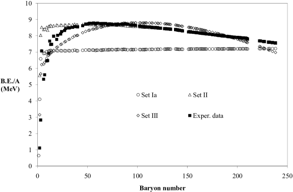
Figure 1: Ratio of the binding energy ($B.E.$) over the atomic number $A$ (or baryon number) as a function of $A$. The experimental data (black squares) are shown along with predicted value for parametization of Set Ia (empty circles), II (empty triangles) and III (empty diamonds) respectively.

where $F^{\prime}=\partial F/\partial u$ and the energy can be expressed in units of $\frac{3\lambda\mu}{4}$. For example for Set II (Set III), the nonlinear $\sigma$ term is proportional to $\alpha\left(\frac{4}{3\lambda\mu^{2}}\right)^{\frac{2}{3}}=3.73524\times 10^{-7}$ $(1.43418\times 10^{-6})$ and the Skyrme term to $\beta\left(\frac{16}{9\lambda^{2}\mu}\right)^{\frac{2}{3}}=-1.3263\times 10^{-6}$ $(-9.2355\times 10^{-6})$ while the remaining terms are of order one. Furthermore the overall factor $\left(\frac{3\lambda\mu}{4}\right)$ remains approximately the same for all the sets. Looking at the numerical results, we observe nonetheless that these two terms are responsible for corrections of the order of $0.01\%.$ Clearly, the small magnitude of these contributions provides support to the assumption that (40) is a good approximation to the exact solution.

Comparing Set II to the original Skyrme Model with a pion mass term, we may identify

$$F_{\pi} =4\sqrt{\alpha}=0.364474\text{ MeV\qquad(Experiment: }F_{\pi}=\text{186 MeV)}$$

$$e^{2} =\frac{1}{32\beta}=-57019\qquad\text{(}e=4.84\text{ for massive pion Skyrme Model)}$$

$$m_{\pi} =\frac{2\sqrt{\alpha}}{\mu}=231591\text{ MeV\qquad(Experiment: }m_{\pi}=\text{138 MeV)}$$

Set III leads to similar values for $F_{\pi},e^{2}$ and $m_{\pi}$ which are orders of magnitude away for the usual values obtained for the Skyrme model. Of course here the nonlinear $\sigma$ and Skyrme terms do not play a significant role in the stabilization of the soliton. Indeed the Skyrme term even have the wrong sign so it would destabilize the soliton against shrinking if it was not for the contribution of order six in derivatives. The size of the soliton is instead determined by the relative magnitude of $\mu$ and $\lambda$ so there is no need for $F_{\pi}$ and $m_{\pi}$ to be close to the nucleon mass scale as for the original Skyrme Model. Perhaps the explanation for such a departure is that the parameters of the model are merely bare parameters and they could differ significantly from their renormalized physical values. We note also that the $B>1$ solutions of the Skyrme Model display a totally different structure compared to the BPS-type solution analyzed here. It is well known that the lowest-energy $B=2,3,4...$ solutions of the Skyrme Model exhibit respectively toroidal, tetrahedral, cubic,… baryon density configurations. Such solution are conveniently represented by an ansatz based on rational maps Houghton . The model at hand here leads to spherically symmetric baryon density at least in the regime of small $\alpha$ and $\beta$ where solution (40) can apply. So it seems that the regime dominated by the $\mu$ and $\lambda$ terms leads to spherical configurations whereas the regime dominated by the nonlinear $\sigma$ and Skyrme terms shows totally different baryon density distributions. In the absence of a complete analysis, we can only conjecture that the change in configuration is related to which of the four terms are responsible for the stabilization of the soliton and at some critical values of the parameters there is a transition between configurations.

Let us now look more closely at the numerical results presented in Fig. 1. These are in the form of the ratio of the binding energy ($B.E.$) over the atomic number $A$ as a function of $A$ which corresponds to the baryon number. The experimental data (black squares) are shown along with predicted value for parametization of Set Ia (empty circles), II (empty triangles) and III (empty diamonds) respectively. Clearly Set Ia is less accurate when it comes to reproduce the full set of experimental data but is somewhat successful for the lightest nuclei. This to be expected since the fit relies on the masses of the nucleon and ⁴He. Yet all predicted nuclear masses are found to be within a 0.3% precision. In fact the ratio $B.E./A$ is rather sensitive to small variation of the nuclear masses so the results in general are surprisingly accurate. On the other hand Set II, based on the nuclear masses, overestimates the binding energies of the lightest nuclei while it reproduces almost exactly the remaining experimental values. The least square fit based on $B.E./A$, Set III, is the best fit overall but in order to better represent the features of lightest nuclei, it abdicates some of the accuracy found in Set II for $B>30$.

This apparent dichotomy between the description of the two regions $B\leq 30$ and $B>30$ may find an explanation in the (iso)rotational contribution to the mass. Indeed light nuclei have smaller sizes and moments of inertia so that their rotational energy contributes to a larger fraction of the total mass since the spins and isospins remain relatively small. On the other hand the size of heavy nuclei grows as $B^{\frac{1}{3}}$ and their moments of inertia increase accordingly. The spin of the most abundant isotopes are relatively small while isospin can have relatively large values due to the growing disequilibrium between the number of proton and the number of neutron in heavy nuclei (see eq. 50). Despite these behaviors, our numerical results show that the rotational energy is less that 1 MeV for $B>10$ for any of the Sets considered and its contribution to $B.E./A$ decreases rapidly as $B$ increases. On the contrary for $B<10$ the rotational energy is responsible for large part of the binding energy which means that $B.E./A$  should be very sensitive to the way the rotational energy is computed. In our case we approximated the nucleus as a rigid rotator. One may argue that if rotational deformations due to centrifugal effects were to be considered, it would lead to larger moments of inertia and lower rotational energies. This would predominantly affect the binding energy of the lightest nuclei since this is where rotational energy is most significant. Allowing for such deformation would in general require the full numerical computation of the solution. An easier way to check for deformation is by allowing the ratio of the parameters $\sigma=\mu/\lambda$ in the solution (40) to vary independently from the $\mu$ and $\lambda$ in the model (4) and by repeating the fit with respect to five parameters instead of the four previous ones. This procedure allows for a further adjustment of the size of the soliton in terms of $\sigma$ with respect to a given choice of model parameters $\mu,\alpha,\beta$ and $\lambda$ and would lead to partial deformation of the solution. Such a parametrization is expected to increase both the size and the moments of inertia of the soliton and decrease the total mass of the lightest nuclei which would be an improvement over the four parameters fit. We evaluated such correction for the nucleon whose relative contribution to mass from rotation is the largest using the parameters of Set II and we obtained a modest decrease of the mass of the order of 0.16%. Since the rotational energy accounts for much less than 1% of the total energy in most of the nuclei, deformations are not generally expected to be very significant.

VI Conclusion

We have proposed a 4-terms model as a generalization of the Skyrme Model. In the regime where two of the terms are negligible, i.e. $\alpha=\beta=0$, we find well-behaved analytical solutions for the static solitons. These saturate the Bogomolny’s bound with consequence that the static energy is directly proportional to the baryon number $B$. They differ from those obtained by ASW in an important way: their model lead to compactons at the boundary of which the gradient of the solution is infinite and so the solution could not be used to approximate the energies in the regime where $\alpha,\beta\neq 0$. Furthermore, one of the major feature of our model is that the form of the solutions allows to compute analytically the static and rotational energy and express them as a function of the model parameters and $B$. Fixing the remaining parameters of the model, $\mu$ and $\lambda,$ leads to rather accurate predictions for the mass of the nuclei.

We then used these BPS-type solutions to compute the mass of the nuclei in the regime where $\alpha$ and $\beta$ are small but not zero. Indeed fitting the model parameters to provide the best description of the nuclear mass data leads to that particular regime where the values of $\alpha$ and $\beta$ turn out to be very small. Yet we find a noticeable improvement in the size and $B.E./A$ predictions with respect to those for the $\alpha=\beta=0$ regime. Even though our 4-term model can be considered a simple extension of the massive pion Skyrme Model (different mass term and an additional term with six derivatives in pion fields) the solution leads to spherically symmetric baryon densities as opposed to more complex configurations for $B>1$ standard Skyrmions (e.g. toroidal, tetrahedral, cubic…). These results suggest that nuclei could be considered as near BPS-Skyrmions.

This work was supported by the National Science and Engineering Research Council of Canada.

References

- (1) T.H.R. Skyrme, Proc. Roy. Soc. Lond. A, 260:127-138, 1961; T.H.R. Skyrme, Proc. Roy. Soc. Lond. A, 247:260–278, 1961; T.H.R. Skyrme, Nucl. Phys. 31:556-569, 1962; T.H.R. Skyrme, Proc. Roy. Soc. Lond. A, 247:260–278, 1958.
- (2) G. t Hooft, Nuclear Physics B, 72:461-473, 1974.
- (3) E. Witten, Nuclear Physics B, 160:57-115, 1979.
- (4) L. Marleau, Phys. Rev. D, 43:885-890, 1991.
- (5) E. Bonenfant and L. Marleau, Phys. Rev. D, 80:114018, 2009.
- (6) V. B. Kopeliovich, B. Piette and W. J. Zakrzewski, Phys. Rev. D, 73:014006, 2006.
- (7) P. Sutcliffe, Phys. Rev. D, 79:085014, 2009.
- (8) G. S. Adkins and C. R. Nappi, Phys. Lett. B, 137:251-256, 1984.
- (9) C. J. Houghton, N. S. Manton and P. M. Sutcliffe, Nucl. Phys. B, 510:507-537, 1998.
- (10) J.-P. Longpré and L. Marleau, Phys. Rev. D, 71:095006, 2005.
- (11) C. Houghton and S. Magee, Physics Letters B, 632:593-596, 2006.
- (12) C. Adam, J. Sanchez-Guillen and A. Wereszczynski, arXiv : 1001.4544, 2010.
- (13) G. S. Adkins and C. R. Nappi, Nucl. Phys. B, 233:109-115, 1984.
- (14) P. Sutcliffe, arXiv : 1003.0023, 2010.
- (15) See for example K. S. Krane, Introductory Nuclear Physics, John Wiley and sons, p. 67, 1987 or more recent G.Audi, A.H.Wapstra and C.Thibault, Nuclear Physics A729,337-676 (2003).
- (16) J. Fortier and L. Marleau, Phys. Rev. D, 77:054017, 2008.
- (17) V. G. Makhankov, Y. P. Rybakov and V. I. Sanyuk, Springer, 1993.