An uncertainty principle underlying the pinwheel structure in the primary visual cortex
1 Introduction
The visual information in V1 is processed by an array of modules called orientation preference columns [1]. In some species including humans, orientation columns are radially arranged around singular points like the spokes of a wheel, that are called pinwheels. The pinwheel structure has been observed first with optical imaging techniques [2] and more recently by in vivo two-photon imaging proving their organization with single cell precision [3]. Many hypotheses of morphogenesis of pinwheels during visual development have been proposed e.g. [4][5] and many reviewed in [6][7], but at the present the problem is still open [8]. In this research we do not intend to propose another model of pinwheel formation, but instead provide evidence that pinwheels are de facto optimal distributions for coding at the best angular position and momentum. In the last years many authors have recognized that the functional architecture of V1 is locally invariant with respect to the symmetry group of rotations and translations [9][10][11][12][13][14][15]. In the present study we show that the orientation cortical maps measured in [2] to construct pinwheels, can be modeled as coherent states, i.e. the geometric configurations best localized both in angular position and momentum. The theory we adopt is based on the well known uncertainty principle, first proved by Heisenberg in quantum mechanics [16], and later extended to many other groups of invariance [17][18][19]. This classical principle states an uncertainty between the two noncommutative quantities of linear position and linear momentum and it has been adopted in [20] to model receptive profiles of simple cells as minimizers defined on the retinal plane. Here we state a corresponding principle in the cortical geometry with symmetry based on the uncertainty between the two noncommutative quantities of angular position and angular momentum. By computing its minimizers we obtain a model of orientation activity maps in the cortex. As it is well known the pinwheels configuration is directly constructed from these activity maps [2], and we will be able to formally reproduce and justify their structure, starting from the group symmetries of the functional architecture of the visual cortex. The primary visual cortex is then modeled as an integrated system in which the set of simple cells implements the group, the horizontal connectivity implements its Lie algebra and the pinwheels implement its minimal uncertainty states.
2 The functional architecture of V1
2.1 Simple cells as elements of a phase space
Receptive fields of simple cells of the area V1 are classically represented as Gabor-like filters able to accomplish an analysis both in space and frequency [20][21][22]. Each filter is identified by four parameters where are coordinates in the D cortical layer , and are the engrafted variables in the sense of Hubel [23]. The coordinate codes the modulus of frequency and the orientation preference, so that they can be interpreted as a choice of polar coordinates in the frequency variables. Since the variables of position and frequency are constitutive of the phase space, the set of simple cells is classically labeled by parameters of a 4D phase space which represents the cotangent space of the 2D cortical layer. We also explicitly note that Gabor filters are complex valued, so that the cortical signals related to this cells are also complex.

2.2 Horizontal connectivity and integral curves in
Simple cells are connected by means of the horizontal connectivity with its typical anisotropic pattern described in detail in a number of experiments (e.g. [25]). It has been shown that the functional architecture of cortico-cortical connections among simple cells strongly depends on position and orientation preference, while it presents a weaker dependence on the frequency. Indeed, while studying the connectivity, very often in literature only the three parameters are considered, while the modulus of frequency is discarded [9][12][10][15]. Moreover, the functional architecture is invariant for change of polarity of simple cells so that the variable is defined on , instead of . Hence the polar coordinates will be expressed as . These parameters are the coordinates of the reduced cotangent space which can be identified with the elements of the group of translations and rotations of , representing the group of symmetries of the functional architecture of V1.
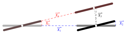
The group acts on a vector applied in the origin by rotating it of an angle and by translating its application point of :
| (1) |
where
In particular is the 2D projection of the group action.
The tangent space of has dimension three and it is generated by the infinitesimal transformations along two orthogonal translations and the rotation of the group. However, in order to take into account the anisotropy of the connectivity, in [12] and [26] just two generators instead of three were considered. In particular in [12] it was proposed to choose as generators the differential operators and representing only one infinitesimal translation and the infinitesimal rotation. Projecting them on the 2D cortical layer through the local action defined in (1) we obtain
and
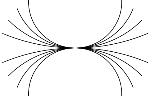
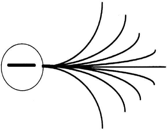
These derivations are left invariant with respect to the action and are simply the directional derivatives in the direction respectively and . The horizontal connectivity is then modeled as the set of integral curves of the vector fields having starting point at the origin of the local coordinates and varying the parameter in (see Fig. 1(b)):
Computing the left invariant derivatives at the point amounts to choose local coordinates around a fixed point. This is why the fan is centered in the origin and oriented along the -axis in local coordinates. However this choice is not restrictive, since we can always apply the action and recover global coordinates, in which the fan has an arbitrary origin and direction . Hence, in the sequel, we will always make this choice of local coordinates.
The cortical activity defined on the 2D cortical layer is propagated along the horizontal long range connectivity, modeled by the -curves so that the gradient of the cortical activity will be computed as directional derivative of along the vector fields and .
2.3 The operators in the reduced Fourier domain
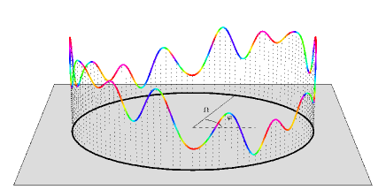
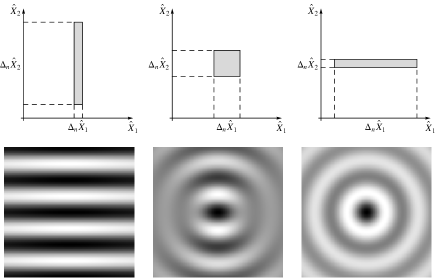
The reduced phase space contains all the position variables but only the angular component of the frequency variable. Hence in the Fourier space it supports only functions defined on a semicircle of radius fixed, and periodical of period as depicted in Fig 2(a). The operators acting on these functions are the Fourier transforms of and :
| (2) |
Let us note that the fields and correspond respectively to angular position and angular momentum of the periodic quantum pendulum [16]. The parameter is specified by the physics of the problem and in our case it will express the reciprocal of the correlation length of pinwheels in accordance with [27].
3 An uncertainty principle on the functional geometry
3.1 The noncommutativity of vector fields
While studying the relation between angular position and momentum, both in the real and Fourier plane, we have to take into account that the composition of a translation and a rotation is not commutative:
The difference for sufficiently small is an increment in the direction orthogonal to (see Fig. 2(b)). This property implies the non commutativity of left invariant derivatives and . In particular if we compute second mixed derivatives we have that We will call commutator of and the difference which is a measure of the non commutativity of the space. The same property can be transferred in the transformed fields and whose commutator is
3.2 The uncertainty principle
This noncommutative framework has important analogies with the canonical quantum mechanical case, in which the two non commuting operators are position and momentum. In that specific situation the variance of the position and momentum operators on functions have a lower bound that has been formalized in the well known Heisenberg uncertainty principle. This principle has been formally extended (see [17] and references therein) to general non commuting vector fields. Hence we can express here a similar uncertainty principle in terms of the vector fields and
| (3) |
where is the standard deviation of the operator and is the mean value of the operator when evaluated on the function . For fixed we recognize that, if is concentrated in the Fourier domain so that its variance is small, then the variance of the angular momentum has to be high and viceversa. Note that the inequality expresses the uncertainty principle for the periodic quantum pendulum between the two observable angular position and angular momentum. For , the fields and reduce to the classical position and momentum operators of the harmonic oscillator and the inequality expresses the well known Heisenberg uncertainty principle.
4 Coherent states as optimal localization in angular position and angular momentum
4.1 Coherent states in the Fourier space
The minimizers of the uncertainty principle are called coherent states and correspond to the functions with the optimal localization in angular position and angular momentum. Let us first compute the reference minimal uncertainty “ground” state by making use of the well-known equation (see [17])
| (4) |
where the scaling parameter represents the frequency of the pendulum. Its solution can be analytically computed and, up to a normalization constant, is the ground state . The set of coherent states of in the Fourier domain depends on the angular parameter and is obtained as a displacement of the ground state of an angle :
| (5) |
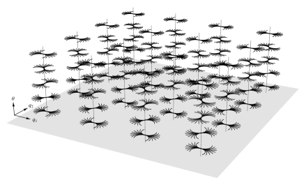
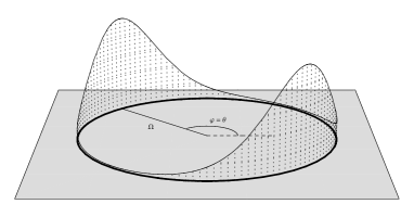
Every coherent state represents the most concentrated function for optimal localization in angular position and momentum, both taken starting from the reference angle . The function is bell-shaped and centered around the angle (see Fig. 3(a)). We note that the bigger is , the sharper is its localization. Indeed its standard deviation can be evaluated as and its width reduces around as becomes big, leading to a delta in the limit.
If then and the variance of the angular position is null, meaning that it is maximally concentrated. Due to the uncertainty inequality has infinite variance i.e. it is maximally undetermined. On the other hand, if is constant, then and the angular momentum is maximally concentrated.
Up to now, the coherent states have been computed using left invariant operators of the group and hence imposing invariance on the domain of functions. Now we impose invariance also on the co-domain of with respect to local phase rotation so that each function is a coherent state. These states are solutions of the equation (4) where the operators and are expressed in terms of covariant derivatives instead of the usual derivatives. These coherent states, visualize in Fig 3(c) are invariant for any local change of coordinates in the domain and co-domain, modeling a system that does not require any knowledge of an external global reference system.
4.2 Coherent states in the real plane
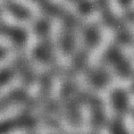
The Fourier anti-transform of the function defined on a circle of radius gives the expression of the coherent states in the real plane, providing the maps visualized in figure.
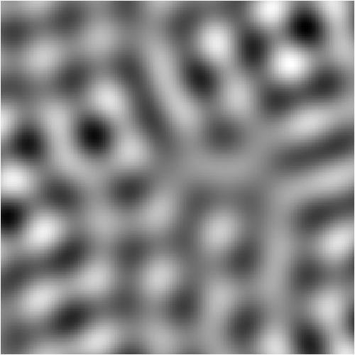
4.3 From coherent states to pinwheels
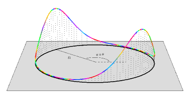
In [2] the pinwheel structure of V1 has been reconstructed starting from a set of cortical activity maps acquired with optical imaging techniques in response to gratings with different orientations . A color image has been obtained from gray valued activity maps, associating a color coding representation to preferred orientations [28]. Here we apply the same procedure to the set of coherent states (our model of activity maps), producing the pinwheel structure visualized at the center of Fig. 4.
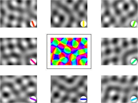
5 Qualitative and quantitative comparison with orientation cortical maps
The image show a qualitative impressive similarity with the original result obtained in [2] [29] [25] among many others. Moreover by computing the power spectrum of recorded pinwheels, following [27], a function defined on an annulus with radius is obtained, in complete accordance with the result predicted by the presented theory, built up on the basis of the geometry of the functional architecture. In our perspective the orientation activity maps are modeled by the coherent states, minimizing uncertainty introduced by functional geometry. Note that the coherent states are periodic as the measured activity maps. To our knowledge in the existing models of pinwheels the activity maps are obtained a posteriori, while in our approach a geometric model of the activity maps is directly provided and the pinwheels are constructed as in the classical experiments.
References
- [1] D. H. Hubel and T. N. Wiesel. Ferrier lecture: Functional architecture of macaque monkey visual cortex. Royal Society of London Proceedings Series B, 198:1–59, May 1977.
- [2] T. Bonhoeffer and A. Grinvald. Iso-orientation domains in cat visual cortex are arranged in pinwheel-like patterns. Nature, 353(6343):429–431, October 1991.
- [3] K. Ohki, S. Chung, P. Kara, M. Hubener, T. Bonhoeffer, and R. C. Reid. Highly ordered arrangement of single neurons in orientation pinwheels. Nature, 442(7105):925–928, August 2006.
- [4] F. Wolf and T. Geisel. Spontaneous pinwheel annihilation during visual development. Nature, 395(6697):73–78, September 1998.
- [5] P. C. Bressloff and J. D. Cowan. A spherical model for orientation and spatial-frequency tuning in a cortical hypercolumn. Philosophical transactions of the Royal Society of London. Series B, Biological sciences, 358(1438):1643–1667, October 2003.
- [6] N. V. Swindale. The development of topography in the visual cortex: a review of models. Network (Bristol, England), 7(2):161–247, May 1996.
- [7] H. D. Simpson, D. Mortimer, and G. J. Goodhill. Theoretical models of neural circuit development. Current topics in developmental biology, 87:1–51, 2009.
- [8] A. D. Huberman, M. B. Feller, and B. Chapman. Mechanisms underlying development of visual maps and receptive fields. Annual Review of Neuroscience, 31(1):479–509, 2008.
- [9] O. Ben-Shahar and S. Zucker. Geometrical computations explain projection patterns of long-range horizontal connections in visual cortex. Neural Computation, 16(3):445–476, March 2004.
- [10] J. Zweck and L. R. Williams. Euclidean group invariant computation of stochastic completion fields using shiftable-twistable functions. Journal of Mathematical Imaging and Vision, 21(2):135–154, September 2004.
- [11] P. C. Bressloff, J. D. Cowan, M. Golubitsky, P. J. Thomas, and M. C. Wiener. Geometric visual hallucinations, euclidean symmetry and the functional architecture of striate cortex. Philosophical Transactions of the Royal Society of London. Series B: Biological Sciences, 356(1407):299–330, March 2001.
- [12] G. Citti and A. Sarti. A cortical based model of perceptual completion in the roto-translation space. Journal of Mathematical Imaging and Vision, 24(3):307–326, May 2006.
- [13] E. Franken and R. Duits. Crossing-preserving coherence-enhancing diffusion on invertible orientation scores. International Journal of Computer Vision, 85(3):253–278, December 2009.
- [14] A. Sarti, G. Citti, and J. Petitot. The symplectic structure of the primary visual cortex. Biological Cybernetics, 98(1):33–48, 2008.
- [15] R. Duits, M. Felsberg, G. Granlund, and B. Romeny. Image analysis and reconstruction using a wavelet transform constructed from a reducible representation of the euclidean motion group. International Journal of Computer Vision, 72(1):79–102, April 2007.
- [16] C. Cohen-Tannoudji, B. Diu, and F. Laloe. Quantum Mechanics. John Wiley & Sons, June 1978.
- [17] G. Folland. Harmonic analysis on phase space. Princeton University Press, 1989.
- [18] P. Carruthers and M. M. Nieto. Phase and angle variables in quantum mechanics. Reviews of Modern Physics, 40(2):411–440, Apr 1968.
- [19] C. J. Isham and J. R. Klauder. Coherent states for n-dimensional euclidean groups e(n) and their application. Journal of Mathematical Physics, 32(3):607–620, 1991.
- [20] J. G. Daugman. Uncertainty relation for resolution in space, spatial frequency, and orientation optimized by two-dimensional visual cortical filters. J. Opt. Soc. Am. A, 2(7):1160–1169, July 1985.
- [21] T. S. Lee. Image representation using 2d gabor wavelets. IEEE Transactions on Pattern Analysis and Machine Intelligence, 18(10):959–971, 1996.
- [22] J. P. Jones and L. A. Palmer. An evaluation of the two-dimensional gabor filter model of simple receptive fields in cat striate cortex. J Neurophysiol, 58(6):1233–1258, December 1987.
- [23] David H. Hubel. Eye, Brain, and Vision (Scientific American Library, No 22). W. H. Freeman, 2nd edition, May 1995.
- [24] D. J. Field, A. Hayes, and R. F. Hess. Contour integration by the human visual system: Evidence for a local association field. Vision Research, 33:173–193, 1993.
- [25] B. Schofield W. H. Bosking, Y. Zhang and D. Fitzpatrick. Orientation selectivity and the arrangement of horizontal connections in tree shrew striate cortex. J. Neurosci., 17(6):2112–2127, March 1997.
- [26] J. Petitot and Y. Tondut. Vers une neurogéométrie. fibrations corticales, structures de contact et contours subjectifs modaux, 1999.
- [27] E. Niebur and F. Wörgötter. Design principles of columnar organization in visual cortex. Neural Computation, 6(4):602–614, July 1994.
- [28] N. V. Swindale, J. A. Matsubara, and M. S. Cynader. Surface organization of orientation and direction selectivity in cat area 18. J. Neurosci., 7(5):1414–1427, May 1987.
- [29] G. G. Blasdel. Orientation selectivity, preference, and continuity in monkey striate cortex. J. Neurosci., 12(8):3139–3161, August 1992.