Coherence as ultrashort pulse train generator

Abstract

Intense, well-controlled regular light pulse trains start to play a crucial role in many fields of physics. We theoretically demonstrate a very simple and robust technique for generating such periodic ultrashort pulses from a continuous probe wave which propagates in a dispersive thermal gas media.

I
Introduction

The invention of the optical frequency comb has revolutionized optical frequency metrology [1-4]. Today it is playing an important role in high resolution spectroscopy [5],the spectral purity and large bandwidth of optical frequency combs provides also means for the precise control of generic quantum systems such as laser cooling of molecules or exotic atomic species [6,7], and quantum state engineering in molecules [8-10].  Optical frequency comb is becoming a crucial component in the field of quantum information science, where complex multilevel quantum systems must be controlled with great precision [10,11] and frequency comb technique promises to become an effective tool in astronomical observations [12].

The usage of quantum interference effects in order to manipulate the optical properties of gaseous atomic or molecular medium has by now been established as a useful and powerful method. In particular in [13] Harris and co-workers have suggested and used a Raman-type three level interaction scheme in D2-molecular gas to get series of femtosecond pulses. In our recent paper [14], discussing propagation of radiation probe wave in a medium of dressed two-level atoms initially prepared in a quantum superpositional state of ground and excited energy levels, we showed that it splits into a sequence of ultrashort pulses with easy and precise tunning of possible control parameters. Later  we will refer to this scheme as QS (quantum superposition) generator.  In general this process can be accompanied by pulse amplification. It may be interesting, in addition, that the gas refractive index in comparison with earlier known results contains out of dipole approximation terms of resonant nature which have no saturation in dependence on pump wave intensity [15].

In this Paper, we bring the QS generator problem discussion  closer to real experimental settings. As a crucial point on this path we see the manner of (superposition) state preparation.  The most convenient way to embody the superposition, is rapid switching  on of the dressing field.  It does not require additional  perturbing sources in the experimental setup and gives  number of parameters (such as the switching time, pump wave intensity and resonance detuning) to regulate the superposition.  We present  here the whole chain, starting from coherent state preparation and finishing with incident wave modulation. We show that under appropriate conditions, spontaneous emission and Doppler broadening have small impact on the comb generation process.

II The Model

So we consider a gas of two-level atoms with energy difference $\hbar\omega_{0}$ between the excited and ground internal atomic bare states $\left|2\right\rangle$ and $\left|1\right\rangle$ in a far off-resonance field of the pump field

$$\text{ }E_{pump}(z,t)=\text{ }\varepsilon_{pump}(z,t)\exp[ik_{pump}z-i\omega_{pump}t]+c.c.\text{,}$$ (1)

where $\omega_{pump}$ is the carrying frequency of the pump field, $k_{pump}=\omega_{pump}/c$ and $\varepsilon_{pump}(z,t)$ is the slowly varying field amplitude. The spin of relevant to optical transition electron and the possible sublevel structures are not taken into account.  For the pump field amplitude we will take a functional form

$$\varepsilon_{pump}(z,t)=\frac{\varepsilon_{0}}{1+e^{-(t-z/c)/T}}\text{,}$$ (2)

which means that the pump field has a switching front characteristic duration $T$ and travels from left to right  along the $z$ axis. The interaction Hamiltonian $V$ in dipole and rotating wave approximations will reproduce the functional form given in (2).  This form is close to real experimental pulse turn-on process and what is not less important the atom-field interaction problem has an analytical solution for it [16]. The atomic wavefunction is given by

$$\left|\Psi(z,t)\right\rangle_{pump}=f(t-z/c)\left|1\right\rangle e^{-\frac{i}{\hbar}E_{1}t}+g(t-z/c)\left|2\right\rangle e^{-\frac{i}{\hbar}E_{2}t}$$ (3)

with

$$f(t-z/c)=(1-u)^{\sigma}F(a,b;c;u)\text{,}$$ (4)

$$g(t-z/c)=e^{i(kz+\Delta t)}((1-u)^{\sigma}F(a,b,c;u)-(1-u)^{\sigma+1}F(a+1,b+1;c+1;u))\text{,}$$ (5)

where $E_{1}$ and $E_{2}$ are energies of corresponding bare states, $\Delta=\omega_{pump}-\omega_{0}$, $\sigma=-iV_{0}T$, $u=-e^{-t/T}$, $a=(iT/2)\left(-\Delta-2V_{0}+\sqrt{\Delta^{2}+4V_{0}^{2}}\right)$, $b=(iT/2)\left(-\Delta-2V_{0}-\sqrt{\Delta^{2}+4V_{0}^{2}}\right)$ and $c=-i\Delta T$ .

Propagation of a weak probe field through a medium of atoms can be described by wave equation

$$\left(\nabla^{2}-\frac{1}{c^{2}}\frac{\partial^{2}}{\partial t^{2}}\right)E_{probe}(\overrightarrow{r},t)=\frac{4\pi\rho}{c^{2}}\frac{\partial^{2}}{\partial t^{2}}\left\langle\widehat{d}\right\rangle_{probe}\text{.}$$ (6)

$\rho$ is the atom number density and $\left\langle\widehat{d}\right\rangle_{probe}$ is the atomic dipole moment induced by a probe field. To acquire the latter, one has to find first the atomic state $\left|\Psi(z,t)\right\rangle$ in a combined field of pump(dressing) and probe fields, then implement the ordinary quantum mechanical averaging of the dipole operator by means of this state vector, and later select terms proportional to the probe field $E_{probe}(\overrightarrow{r},t)$. The probe field is $E_{probe}(\overrightarrow{r},t)=\epsilon_{0}(\overrightarrow{r},t)\exp[i\overrightarrow{k}\overrightarrow{r}-i\omega t]+c.c.$ with slowly varying amplitude $\epsilon_{0}(\overrightarrow{r},t)$.

The atomic state vector in combined (pump + probe) field has the form

$$\left|\Psi(z,t)\right\rangle=\left|\Psi(z,t)\right\rangle_{pump}+\left|\Delta\Psi(z,t)\right\rangle=(f(t)+C_{1}(z,t))\left|1\right\rangle e^{-\frac{i}{\hbar}E_{1}t}+(g(t)+C_{2}(z,t))\left|2\right\rangle e^{-\frac{i}{\hbar}E_{2}t}\text{,}$$ (7)

where $f(t-z/c)$ and $g(t-z/c)$ are the above determined probability amplitudes in pump laser field.  The additional terms $C_{1}(\overrightarrow{r},t)$ and $C_{2}(\overrightarrow{r},t)$ arise due to interaction with probe radiation and are proportional to the probe field intensity in frame of linear theory.  Note that in distinction from [14], where the pump field was assumed to be strictly monochromatic, here the problem of atomic states in the field of pump radiation is time dependent.

Also it should be noted here that in the asymtotic case when $t-z/c>>T$

$$f(t-z/c)\approx\exp\left[\left(\frac{t-z/c}{T}\right)\left(-iV_{0}T-a\right)\right]h_{1}+\exp\left[\left(\frac{t-z/c}{T}\right)\left(-iV_{0}T-b\right)h_{2}\right]$$

$$g(t-z/c)\approx e^{-i\Delta(t-z/c)}\exp\left[\left(\frac{t-z/c}{T}\right)\left(-iV_{0}T-a\right)\right](h_{1}-h_{3})+\exp\left[\left(\frac{t-z/c}{T}\right)\left(-iV_{0}T-b\right)h_{2}\right](h_{2}-h_{4})$$

with $h_{1}=\Gamma(c)\Gamma(b-a)/\Gamma(b)\Gamma(c-a)$, $h_{2}=\Gamma(c)\Gamma(a-b)/\Gamma(a)\Gamma(c-b)$, $h_{3}=\Gamma(c+1)\Gamma(b-a)/\Gamma(b+1)\Gamma(c-a)$, $h_{4}=\Gamma(c+1)\Gamma(a-b)/\Gamma(a+1)\Gamma(c-b\dot{)}$. So the switching on of the field brings to formation of 4 adiabatic terms, which have different energies in distinction to the case discussed in [14] where were assume only 2 terms with different energies.

The Hamiltonian in dipole approximation is:

$$\widehat{H}=\widehat{H}_{0}-\widehat{\overrightarrow{d}}\overrightarrow{\text{ }E}_{pump}-\widehat{\overrightarrow{d}}\overrightarrow{\text{ }E}_{probe}$$ (8)

After standard calculations in frame of Schrődinger equation, for $C_{1}(\overrightarrow{r},t)$ and $C_{2}(\overrightarrow{r},t)$ amplitudes we obtain

$$C_{1}(\overrightarrow{r},t)=\frac{i}{\hbar}\overrightarrow{d}_{12}\left(e^{i\overrightarrow{k}\overrightarrow{r}}\sigma_{1}(t)\overrightarrow{\varepsilon}_{0}(t)+e^{-i\overrightarrow{k}\overrightarrow{r}}\sigma_{2}(t)\overrightarrow{\varepsilon}_{0}^{\ast}(t)\right)$$ (9)

and

$$C_{2}(\overrightarrow{r},t)=\frac{i}{\hbar}\overrightarrow{d}_{12}^{\ast}\left(e^{i\overrightarrow{k}\overrightarrow{r}}\theta_{2}(t)\overrightarrow{\varepsilon}_{0}(t)+e_{2}^{-i\overrightarrow{k}\overrightarrow{r}}\theta_{1}(t)\overrightarrow{\varepsilon}_{0}^{\ast}(t)\right)\text{,}$$ (10)

where

$$\left\{\sigma_{1},\theta_{1}\right\}={\displaystyle\int\limits_{t_{0}}^{t}}\left\{\beta,\alpha\right\}\text{ }e^{\mp i(\omega+\omega_{0})t^{\prime}}dt^{\prime}\text{,}$$

$$\{\sigma_{2},\theta_{2}\}={\displaystyle\int\limits_{t_{0}}^{t}}\left\{\beta,\alpha\right\}\text{ }e^{\mp i(\omega-\omega_{0})t^{\prime}}dt^{\prime}\text{,}$$

Insertion of found state vectors (7) into $\left\langle\widehat{d}\right\rangle_{probe}=$ $\left\langle\Psi(z,t)\right|\widehat{d}$ $\left|\Psi(z,t)\right\rangle$ determines the right-hand side of wave Eq.(6) as an explicit function of system parameters, proportional to the probe wave amplitude.

In the next step we apply the well known slowly varying approximation to the left-hand side of equation (6) and thus arrive to its reduced form, which is a first order differential equation for the probe wave amplitude $\epsilon_{0}(\overrightarrow{r},t)$ with partial derivatives in both, space and time variables.  Some of the right-hand side terms of obtained reduced wave equation (rwe) are responsible for hyper-Raman scattering, parametric down conversion and four-wave parametric amplification, respectively. However in this paper these processes will not be considered and we will focus our attention on the main nonparametric propagation process. In familiar formulation this approach, as is well known, leads to determination of the medium refractive index.

Introducing new variables  $\tau=t-(\overrightarrow{k}\overrightarrow{r})/\omega$ and $\eta=$ $(\overrightarrow{k}\overrightarrow{r})/k$, we transform our reduced wave equation into an ordinary equation relative to $\eta$ variable where $\tau$ appears as a parameter and thus rwe can be easily integrated.  Assuming that the incident probe wave repeats the form of the pump one and propagates along the pump direction ($\eta=z$) we arrive to the following simple expression for the seeking probe field amplitude $\epsilon_{0}(z,\tau)$:

$$\epsilon_{0}(z,\tau)=\frac{\epsilon_{0}}{\left(1+e^{-\tau/T}\right)}\exp\left[\frac{2\pi\rho\omega_{0}^{2}}{\hbar c\omega}\left|d_{12}\right|^{2}{\displaystyle\int\limits_{0}^{z}}\left(f^{\ast}(\tau)\theta_{1}(\widetilde{z},\tau)-g(\tau)\sigma_{1}(\widetilde{z},\tau)\right)e^{i(\omega-\omega_{0})(\tau+\widetilde{z}/c)}d\widetilde{z}\right]\text{.}$$ (11)

Expression of $\epsilon_{0}(z,\tau)$ is the main product of this paper. It concretizes the result of [14] in case of time dependent pumping field creating the necessary for QS generator  quantum superposition of ground and excited states from the initial state. The imaginary part of  (11) stipulates a phase modulation, while the real part introduces amplitude modulation and intensity variance of the probe laser beam during the propagation in the medium. On the other hand, the exponent is a periodic function of time and spatial coordinate, which results in a periodic-type modulation of the probe field intensity, accompanied by amplification or weakening in average.

III Results and Conclusion

To conceive roughly the picture of probe wave modulation developing by (11) lets turn to the two-level model of alkali metal gases. The characteristic values of $\left|d\right|^{2}$ for dipole allowed transitions are around $2\times 10^{-34}CGSE$ and sample concentration can be varied in a wide range of $10^{12}-10^{16}cm^{-3}$. Typical line broadening is $10^{7}-10^{8}Hz$ and therefore the lowest allowed in frame of this model value for resonance detuning is $\Delta=2\ast 10^{8}Hz$. A picture of probe wave modulation under some possible conditions is given in Fig. 1. In particular here we have presented the case when $t>>T$, that is when the incident field has stabilized. It shows the ability of the  QS generator  scheme to juxtapose the composition of high repetition ultrashort pulses with essential  amplification in the frame of chosen manner of state preparation.

A close consideration of the exponential in Eq. (11) shows that the regularities of QS generator are very simple and convenient from experimental/applied viewpoint.  The rate of probe wave modulation, for instance, is determined solely by the generalized Rabi frequency $\Omega=\sqrt{\Delta^{2}+4V_{0}^{2}}$. This rate in fact determines the space and time repetition distance  between the pulses: $\Delta t_{repetition}=2\pi/\Omega$ and $\Delta z_{repetition}=c\cdot$ $\Delta t_{repetition}$.  The regime of propagation, amplification or weakening, is determined by the detuning $\omega-$ $\omega_{pump}$ (See Fig.1 in [14]).  This dependence is especially sharp near the scattering resonances. The product of gas density on a single-photon scattering cross section determines the modulation depth. Thus, when in amplification regime, increase of the gas density deepens the modulation and thus results in narrowing of peaks in the train.

To incorporate the damping phenomena into theory we will use a simple method, that is we will add to the transition frequency $\omega_{0}$ in (11) the complex quantity $i\gamma$ where $\gamma$ for discusssed parameters is of the order of $10^{7}Hz$. As long as we have a resonance detuning greater than the line broadening, this procedure describes the damping phenomena very well. Our approach takes into account also the spontaneous damping of excitation.

Another factor which should be taken into account is the Doppler or inhomogeneous broadening of optical transition. In a dilute gas at room or higher temperatures the Doppler linewidth prevails the natural and collisional linewidths. We assume a Maxwell-Boltzmann velocity distribution in laser propagation direction.  To actually calculate the influence  of Doppler broadening we should add $\Delta_{Doppler}$ to the detuning and then average over the velocity distribution [17]. The results of these calculations carried out for the same conditions as in Fig.1, and including the relaxation process and the Doppler broadening, prove our assertion that relaxations have minor role in QS generator when far from homogeneous broadening of spectral lines and that the Doppler broadening can not destroy the pulse train formation under appropriate conditions.

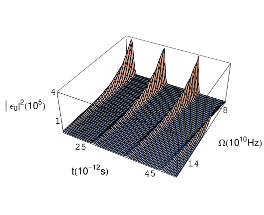
Figure 1: Modulation and amplification of the probe wave in a two-level media.  Here $\Delta=-5\times 10^{12}Hz$, $\omega_{0}=10^{15}Hz$, $\omega-\omega_{0}=5.004\times 10^{11}Hz$,$\rho=10^{15}cm^{-3}$ $z=i\pi c/(b-a)$ and switching characteristic duration $T$ is $10^{-12}s.$

In conclusion, we have shown that  the rapid switching-on of the pump field intensity in a two-level atomic medium may ensure a mixing of adiabatic terms in a way sufficient for formation of the QS generator. The repetition rate and duration of pulses are easily regulated by means of smooth changing of the pump field resonance detuning  and atomic concentration respectively.  Numerical calculations  (for alkali metal vapors) show that the presented mechanism of QS generator of ultrashort pulses is robust against  the homogeneous and inhomogeneous broadening of spectral lines in a very wide range of parameters, as well as parameter fluctuations.

Acknowledgement 1

Authors thank Atom Zh. Muradyan for helpful discussions.  This work was supported by Alexander von Humboldt foundation and Armenian Science Ministry Grant 143.

References

- (1) G. Steinmeyer et al. Science 286, 1507 (1999).
- (2) S. T. Cundiff and J. Ye. Rev. Mod. Phys. 75, 325 (2003).
- (3) J. L. Hall. Rev. Mod. Phys. 78, 1279 (2006).
- (4) T. W. Hansch. Rev. Mod. Phys. 78, 1297 (2006).
- (5) M. C. Stowe et al. Adv. At. Mol. Opt. Phys. 55, 1 (2008).
- (6) D. Kielpinski. Phys. Rev. A 73, 063407 (2006).
- (7) M. Viteau et al. Science 321, 232 (2008).
- (8) A. Pe’er et al. Phys. Rev. Lett. 98, 113004 (2007).
- (9) E. A.Shapiro et al. Phys. Rev. Lett. 101, 023601 (2008).
- (10) Special issue: Quantum Coherence, Nature 453, 1003 (2008).
- (11) D. Hayes et al, Phys. Rev. Lett. 104, 140501 (2010).
- (12) T. Steinmetz et al. Science 321, 1335 (2008).
- (13) S. E. Harris and A. V. Sokolov, Phys. Rev. Lett. 81, 2894 (1998).
- (14) G. Muradyan and A.Zh. Muradyan, Phys. Rev. A 80, 035801 (2009).
- (15) G. Muradyan and A. Zh. Muradyan, J. Mod. Opt. 55, 3581 (2008).
- (16) E.E.Nikitin, Optika i Spektroskopia, 13, 761(1962).
- (17) W. Demtröder, Laser Spectroscopy: Basics Concepts and Instrumentation (Springer, Berlin, 1996).