Climate tipping as a noisy bifurcation: a predictive technique

Abstract

It is often known, from modelling studies, that a certain mode of climate tipping (of the oceanic thermohaline circulation, for example) is governed by an underlying fold bifurcation. For such a case we present a scheme of analysis that determines the best stochastic fit to the existing data. This provides the evolution rate of the effective control parameter, the variation of the stability coefficient, the path itself and its tipping point. By assessing the actual effective level of noise in the available time series, we are then able to make probability estimates of the time of tipping. This new technique is applied, first, to the output of a computer simulation for the end of greenhouse Earth about 34 million years ago when the climate tipped from a tropical state into an icehouse state with ice caps. Second, we use the algorithms to give probabilistic tipping estimates for the end of the most recent glaciation of the Earth using actual archaeological ice-core data.

Keywords: climate tipping, slow passage through saddle-node bifurcation, time-series analysis

1 Introduction

One concern of the UN Climate Change Conference in Copenhagen 2009 was the prediction of future climate change, subject, for example, to a variety of carbon dioxide emission scenarios. A particularly alarming feature of any such prediction would be a sudden and (perhaps) irreversible abrupt change called a tipping point (Lenton et al., 2008; Scheffer, 2009). Such events are familiar in nonlinear dynamics, where they are called (dangerous) bifurcations, at which one form of behaviour becomes unstable and the system jumps rapidly to a totally different ‘steady state’. Many tipping points, such as the switching on and off of ice-ages, are well documented in paleoclimate studies over millions of years of the Earth’s history.

There is currently much interest in examining climatic tipping points, to see if it is feasible to predict them in advance using time-series data derived from past behaviour. Assuming that tipping points may well be governed by a bifurcation in an underlying dynamical system, recent work looks for a slowing down of intrinsic transient responses within the data, which is predicted to occur before most bifurcational instabilities (Held and Kleinen, 2004; Livina and Lenton, 2007). This is done, for example, by determining the propagator, which is estimated via the correlation between successive elements of the time series, in a window sliding along the time series. This propagator is a measure for the linear stability. It should increase to unity at tipping.

Many trial studies have been made on climatic computer models where an arbitrary time, $t=T$, can be chosen to represent ‘today’. The challenge is then to predict a future critical time, $t^{C}>T$, at which the model will exhibit a tipping instability, using only the time history of some variable (average sea temperature, say) generated by the model before time $T$. The accuracy of this prediction can then be assessed by comparing it to the actual continued response of the simulation beyond time $T$. In some cases these trials have been reasonably successful.

Much more challenging, and potentially convincing, is to try to predict real ancient climate tippings, using their preceding geological data. The latter would be, for example, re-constituted time-series provided by ice cores, sediments, etc. Using this data, the aim would be to see to what extent the actual tipping could have been accurately predicted in advance.

One past tipping point that has been analysed in this manner (Livina and Lenton, 2007) is the end of the Younger Dryas event, about 11,500 years ago, when the Arctic warmed by 7° C in 50 years. These authors used a time series derived from Greenland ice-core paleo-temperature data. A second such study (one of eight made by Dakos et al. (2008), using data from tropical Pacific sediment cores, gives an excellent prediction for the end of ‘greenhouse’ Earth about 34 million years ago when the climate tipped from a tropical state into an icehouse state.

After a review of recent research on tipping we study in Section 5 the saddle-node normal form with a drifting normal form parameter and with additive Gaussian noise to determine the probability (or rate) of early noise-induced escape from the potential well depending on the drift speed of the normal form parameter and the noise amplitude.

We show how one can extract the relevant normal form quantities from a given time series. This allows one to adjust predictions of tipping events based on the propagator to take into account the probability of early escape. We demonstrate how it is possible to estimate the probability of noise-induced escape from the potential well using two time series: one is an output from a simple stochastic model, the other is a paleo-temperature record from ice-core data. Since the propensity of the system to escape early from its potential well depends only on the order of magnitude of the ratio between drift speed and noise amplitude we expect our estimates to be reasonably robust.

This prediction science is very young, but the above trials on paleo-events seem very encouraging, and we describe some of them more fully below. The prediction of future tipping points, vital to guide decisions about geo-engineering for example, will benefit from the experience drawn from these trials, and will need the high quality data currently being recorded worldwide by climate scientists today.

2 Tipping of the Climate and its Sub-Systems

2.1 Tipping Points

Work at the beginning of this century which set out to define and examine climate tipping (Rahmstorf, 2001; Lockwood, 2001; National Research Council, 2002; Alley et al., 2003; Rial et al., 2004) focused on abrupt climate change: namely when the Earth system is forced to cross some threshold, triggering a sudden transition to a new state at a rate determined by the climate system itself and (usually) faster than the cause, with some degree of irreversibility. Recently, the Intergovernmental Panel on Climate Change (IPCC, 2007) made some brief remarks about abrupt and rapid climate change, while Lenton et al. (2008) have sought to define these points more rigorously. The physical mechanisms underlying these tipping points are typically internal positive feedback effects of the climate system (thus, a certain propensity for saddle-node bifurcations).

2.2 Tipping Elements

In principle a climate tipping point might involve simultaneously many features of the Earth system, but it seems that many tipping points might be strongly associated with just one fairly well defined sub-system. These tipping elements are well-defined sub-systems of the climate which work (or can be assumed to work) fairly independently, and are prone to sudden change. In modelling them, their interactions with the rest of the climate system are typically expressed as a control parameter (or forcing) that varies slowly over time.

Recently Lenton et al. (2008) have listed nine tipping elements that they consider to be primary candidates for future tipping due to human activities, and as such have relevance to political decision making at Copenhagen (2009) and beyond. These elements, their possible outcomes, and Lenton’s assessment of whether their tipping might be associated with an underlying bifurcation are:

• loss of Arctic summer sea-ice (possible bifurcation);

• collapse of the Greenland ice sheet (bifurcation);

• loss of the West Antarctic ice sheet (possible bifurcation);

• shut-down of the Atlantic thermohaline circulation (fold bifurcation);

• increased amplitude or frequency of the El Niño Southern Oscillation (some possibility of bifurcation);

• switch-off of the Indian summer monsoon (possible bifurcation);

• changes to the Sahara/Sahel and West African monsoon, perhaps greening the desert (possible bifurcation);

• loss of the Amazon rainforest (possible bifurcation);

• large-scale dieback of the Northern Boreal forest (probably not a bifurcation).

The analysis and prediction of tipping points of climate subsystems is currently being pursued in several streams of research, and we should note in particular the excellent book by Marten Scheffer about tipping points in ‘Nature and Society’, which includes ecology and some climate studies (Scheffer, 2009).

3 Bifurcations and their Precursors

3.1 Generic Bifurcations of Dissipative Systems

The great revolution of nonlinear dynamics over recent decades has provided a wealth of information about the bifurcations that can destabilise a slowly evolving system like the Earth’s climate. These bifurcations are defined as points during the slow variation of a ‘control’ parameter at which a qualitative topological change of behaviour is observed in the multi-dimensional phase space of the system.

The Earth’s climate is what dynamicists would call a dissipative system, and for this the bifurcations that can be typically encountered under the variation of a single control parameter are classified into three types, safe, explosive and dangerous (Thompson et al., 1994; Thompson and Stewart, 2002).

The safe bifurcations, such as the supercritical Hopf bifurcation, exhibit a continuous supercritical growth of a new attractor path with no fast jump or enlargement of the attracting set. They are determinate with a single outcome even in the presence of small noise, and generate no hysteresis with the path retraced on reversal of the control sweep. The explosive bifurcations are less common phenomena lying intermediate between the safe and dangerous types: we simply note here that, like the safe bifurcations, they do not generate any hysteresis. The dangerous bifurcations are typified by the simple fold (saddle-node bifurcation) at which a stable path increasing with a control parameter becomes unstable as it curves back towards lower values of the control, and by the subcritical bifurcations. They exhibit the sudden disappearance of the current attractor, with a consequential sudden jump to a new attractor (of any type). They can be indeterminate in outcome, depending on the topology of the phase space, and they always generate hysteresis with the original path not reinstated on control reversal.

Any of these three bifurcation types could in principle underlie a climate tipping point. But it is the dangerous bifurcations that will be of major concern, giving as they do a sudden jump to a different steady state with hysteresis, so that the original steady state will not be re-instated even if the controlling cause is itself reversed. So any future climatic tipping to a warmer steady state may be irreversible: a subsequent reduction in CO₂ concentration will not (immediately, or perhaps ever) restore the system to its pre-tipping condition.

3.2 Time-Series Analysis of Incipient Bifurcations

Most of the bifurcations in dissipative systems, including the static and cyclic folds which are the most likely to be encountered in climate studies, have the following useful precursor (see Thompson and Stewart (2002) for more details). The stability and attracting strength of the current steady state is becoming steadily weaker and weaker in one mode as the bifurcation point is approached. This implies that under inevitable noisy disturbances, transient motions returning to the attractor will become slower and slower: in the limit, the rate of decay of the transients decreases linearly to zero along the path.

Held and Kleinen (2004) and Livina and Lenton (2007) have recently presented algorithms that are able to detect incipient saddle-node bifurcations from time series of dynamical systems. Both methods estimate the linear decay rate (LDR) toward a quasi-stationary equilibrium that is assumed to exist and to drift toward a saddle-node bifurcation. Typical test data for the algorithms comes from either archaeological records or from output of climate models. Both algorithms (degenerate finger-printing by Held and Kleinen (2004) and detrended fluctuation analysis by Livina and Lenton (2007)) have to make assumptions about the process underlying the recorded time series that are generally believed to be sensible for the tipping elements listed by Lenton et al. (2008). First, one has to assume that the process is a dynamical system close to a stable equilibrium that drifts only slowly but is perturbed by (random) disturbances. The second assumption is that the system is effectively one-dimensional, that is, the equilibrium of the undisturbed system is strongly stable in all directions except a single critical one. Quantitatively this means that one assumes the presence of three well-separated time scales, expressed as rates:

$$\kappa_{\mathrm{drift}}\ll\kappa_{\mathrm{crit}}\ll\kappa_{\mathrm{stab}}\mbox{.}$$

Here $\kappa_{\mathrm{drift}}$ is the average drift rate of those quantities that the algorithm treats as a parameter, for example, freshwater forcing in studies of the thermohaline circulation (THC, the global heat- and salinity-driven conveyor belt of oceanic water). The rate $\kappa_{\mathrm{crit}}$ is the rate with which a small disturbance in state space relaxes back to equilibrium. The rate $\kappa_{\mathrm{stab}}$ is the decay rate of all other non-critical modes. We note that the drift rate $\kappa_{\mathrm{drift}}$ becomes larger than $\kappa_{\mathrm{crit}}$ once the drifting parameter is very close to its bifurcation value. Third, one assumes that the disturbances are small in the sense that the relaxation to equilibrium is governed mostly by the linear decay rates (this implies, for example, that the potential well in which the dynamical system can be imagined to be sitting is approximately symmetric in the critical direction).

The basic procedure proposed by Held and Kleinen (2004) consists of three steps, given a time series $(t_{k},z_{k})$ of measurements $z_{k}$ at possibly unevenly spaced time points $t_{k}$.

1. Interpolation Choose a stepsize $\Delta t$ satisfying

   $$\kappa_{\mathrm{crit}}\ll\frac{1}{\Delta t}\ll\kappa_{\mathrm{stab}}$$

   and interpolate such that the spacing in time is uniform. Now, one has a new time series

   $$z_{k,\mathrm{new}}=z(k\Delta t)\mbox{,}$$

   evenly spaced in time.

2. Detrending Remove the slow drift of the equilibrium by subtracting a slowly moving average. For example, choose a Gaussian kernel

   $$G_{k}(t)=\frac{1}{\sqrt{2\pi}d}\exp\left(-\frac{1}{2}\frac{(t-k\Delta t)^{2}}{d^{2}}\right)$$

   of bandwidth $d$ satisfying

   $$\kappa_{\mathrm{drift}}\ll\frac{1}{d}\ll\kappa_{\mathrm{crit}}\mbox{,}$$

   and subtract the average

   $$Z(k\Delta t)=\frac{\sum_{i=1}^{N}G_{k}(i\Delta t)z_{i}}{\sum_{i=1}^{N}G_{k}(i\Delta t)}$$

   of $z_{k}$ over the kernel. The result of this is a time series

   $$y_{k}=z_{k}-Z(k\Delta t)$$

   which fluctuates around zero and can be considered as stationary on time scales shorter than $1/\kappa_{\mathrm{drift}}$.

3. Fit LDR in sliding window One assumes that the remaining time series, $y_{k}$, can be modelled by a stable scalar linear mapping disturbed by noise, a so-called AR(1)-model

   $$y_{k+1}=c_{k}y_{k}+\theta\eta_{k}$$ (3.1)

   where $\theta\eta_{k}$ is the instance of a random disturbance of amplitude $\theta$ at time $k\Delta t$ and $c_{k}$ is the propagator, related to $\kappa_{\mathrm{crit}}$ at time $k\Delta t$ via

   $$c_{k}=\exp(-\kappa_{\mathrm{crit},k}\Delta t)\mbox{.}$$

   If one assumes that the disturbances $\eta_{k}$ have a normal distribution and are independent from each other, and that $c_{k}$ is nearly constant on time scales shorter than $1/\kappa_{\mathrm{drift}}$, one can choose a sliding window size $w=2m+1$ satisfying

   $$\kappa_{\mathrm{drift}}\ll\frac{1}{w\Delta t}$$

   and determine the propagator $c_{k}$ by an ordinary least-squares fit of

   $$y_{j+1}=c_{k}y_{j}$$

   over the set of indices $j=k-m\ldots k+m$. An estimate for the noise amplitude $\theta$ can be obtained from the standard deviation of the residual of the linear least-squares fit:

   $$\theta_{k}=\operatorname{stdev}\left([y_{j}-c_{k}y_{j}]_{j=k-m}^{\phantom{j=}k+m}\right)$$

This process will stop when the front end of the last window hits the last data point. Notice that when using paleo-data the end of the analysed time series should be chosen before the tipping point that is the object of the investigation. This choice is essential to prevent data, spurious to our predictions of the pre-tipping behaviour, entering the analysis: it also makes a complete analogy with any attempt to predict future tipping points from data terminating today. Figure 1 illustrates this requirement on the sliding windows (with a time series of length $N=20$ for illustration). It also shows a simple linear extrapolation that one might make in order to predict where tipping occurs.

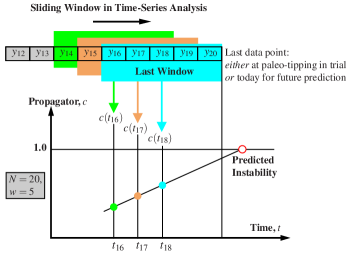
Figure 1: Illustration of sliding windows used in degenerate finger-printing proposed by Held and Kleinen (2004). The extracted autocorrelation coefficient $c_{k}$ is an estimate for the propagator at the mid-time of the sliding windows. Extrapolation is required for prediction.

In this manner Held and Kleinen (2004) obtain the so-called propagator graph of the estimated $c_{k}$ versus its central time, as illustrated in Figure 1. On this graph, $c$ is expected to head towards $+1$ at any incipient bifurcation. In other words, the slowing down of the relaxation from disturbances along the times series can serve as an early-warning signal for an imminent bifurcation (Dakos et al., 2008). We should finally note that having used a first-order mapping in Equation (3.1) and employed autocorrelation techniques, the propagator $c$ is often called the first-order autoregressive coefficient and written as ARC(1). The prediction based on detrended fluctuation analysis, as proposed by Livina and Lenton (2007), also reconstructs the propagator $c$ but does so via the scaling exponent of the variance of the (detrended) time series. For a more complete description of the time-series techniques employed see the recent review by Thompson and Sieber (2010). Also, see Corsi and Taranta (2007) for a discussion of similar problems in power systems engineering (the prediction of fold bifurcations leading to voltage collapse in energy networks).

4 Review of Recent Work

4.1 First Prediction of an Ancient Tipping

The first prediction of an ancient climate tipping event using preceding geological data is due to Livina and Lenton (2007) who tested their detrended fluctuation analysis on the rapid warming of the earth that occurred about 11,500 years ago at the end of the so-called Younger Dryas event (analysing Greenland ice-core paleo-temperature data, which is available from 50,000 years ago to the present).

This Younger Dryas event (Houghton, 2004) was a curious cooling just as the Earth was warming up after the last ice age, as is clearly visible, for example, in records of the oxygen isotope $\delta^{18}O$ in Greenland ice. It ended in a dramatic tipping point, 11,500 years ago, when the Arctic warmed by 7° C in 50 years. Its behaviour is thought to be linked to changes in the thermohaline circulation (THC). This ‘conveyor belt’ is driven by the sinking of cold salty water in the North and can be stopped if too much fresh-melt makes the water less salty, and so less dense. At the end of the ice age when the ice-sheet over North America began to melt, the water first drained down the Mississippi basin into the Gulf of Mexico. Then, suddenly, it cut a new channel near the St Lawrence river to the North Atlantic. This sudden influx of fresh water cut off part of the ocean ‘conveyor belt’, the warm Atlantic water stopped flowing North, and the Younger Dryas cooling was started. It was the re-start of the circulation that could have ended the Younger Dryas at its rapid tipping point, propelling the Earth into the warmer Pre-Boreal era.

The results of Livina and Lenton (2007) are shown in Figure 2, where their propagator (based on detrended fluctuation analysis, DFA) is seen heading towards its critical value of $+1$ at about the correct time. Notice, though, that from a prediction point of view the propagator graph should end at point A when the estimation-window reaches the tipping point. In this example extracting the propagator is particularly challenging because the data set was comparatively small (1586 points) and unevenly spaced.

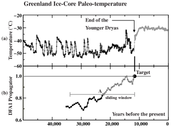
Figure 2: Results of Livina and Lenton (2007): (a) Greenland ice-core (GISP2) paleo-temperature with an unevenly spaced record, visible in the varying density of symbols on the curve. The total number of data points is $N=1586$. In (b) the DFA1-propagator is calculated in sliding windows of length $w=500$ points and mapped into the middle points of the windows. A typical sliding window ending near the tipping is shown.

4.2 Systematic Study of Eight Ancient Tippings

In a more recent paper, Dakos et al. (2008) systematically estimated a propagator stability coefficient from reconstructed time series of real paleo-data preceding eight ancient tipping events. These are:

• the end of the greenhouse Earth about 34 million years ago when the climate tipped from a tropical state (which had existed for hundreds of millions of years) into an icehouse state with ice caps, using data from tropical Pacific sediment cores;

• the end of the last glaciation, and the ends of three earlier glaciations, drawing data from the Antarctica Vostok ice core;

• the Bølling-Alleröd transition which was dated about 14,000 years ago, using data from the Greenland GISP2 ice core;

• the end of the Younger Dryas event about 11,500 years ago, as discussed in the previous section, but drawing not on the Greenland ice core, but rather on data from the sediment of the Cariaco basin in Venezuela;

• the desertification of North Africa when there was a sudden shift from a savanna-like state with scattered lakes to a desert about 5,000 years ago, using the sediment core from ODP Hole 658C, off the west coast of Africa.

In all of the cases studied by Dakos et al. (2008), the propagator $c_{k}$ as extracted by degenerate finger-printing was shown to exhibit a statistically significant increase (corresponding to a slowing down of the relaxation) prior to the tipping transition. Dakos et al. (2008) also demonstrated that their principal result, the statistically significant increase of $c_{k}$, is robust with respect to variations in smoothing kernel bandwidth $d$, sliding window length $w$ and the interpolation procedure.

5 Noise-induced systematic bias of extrapolated prediction

The intention behind the development of the time series analysis algorithms goes beyond statistical evidence of an increasing LDR: the goal of both algorithms is to predict the time (or probability) of the tipping event from the observational data before the event takes place. This is more challenging and suffers from additional uncertainties. Apart from the dependence of the value of $c_{k}$ on algorithm parameters (for example the sliding window length $w$), for a prediction of the time of tipping we have to extrapolate. This implies that we have to assume that the underlying control parameter drifts with nearly constant speed during the recorded time series. This is often not the case in the study of subsystems of the climate when the control parameter is determined by the dynamics of another, coupled, subsystem. Even if the control parameter drifts with constant speed, for prediction we have to assume in addition transversality, that is, the control parameter has to vary the unfolding parameter of the normal form of the saddle-node bifurcation nearly linearly.

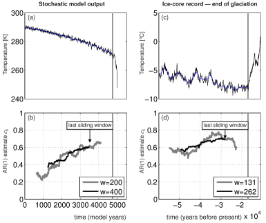
Figure 3: LDR estimates for the output of a model of transition to icehouse earth ((a) and (b)), and for an archaeological temperature record of the end of the recent glaciation ((c) and (d)). See (Petit et al., 1999) and main text for description. Data source: ftp://ftp.ncdc.noaa.gov/pub/data/paleo/icecore/antarctica/vostok/deutnat.txt.

Figure 3 shows two time series ((a) and (c)) and the corresponding time series of extracted estimates for the propagator $c_{k}$ ((b) and (d)). Time series (a) is the output of a model simulation for a transition to an icehouse Earth, and is taken from (Dakos et al., 2008). The model as presented by Dakos et al. (2008) is a scalar stochastic ODE where a control parameter is varied linearly in time and the system is known to encounter a saddle-node bifurcation (originally the model was developed by Fraedrich (1978); see supplement of (Dakos et al., 2008)). Time series (b) shows the propagator $c_{k}$ extracted from time series (a) using degenerate finger-printing. Time series (c) is a snapshot of temperatures before the end of the last glaciation, 20,000 years ago. The data is taken from (Petit et al., 1999), the window of the snapshot is identical to Figure 1(I) in (Dakos et al., 2008). The estimated propagator $c_{k}$ for time series (c) is shown in diagram (d). The graphs in diagrams (b) and (d) are qualitatively the same as in (Dakos et al., 2008) but differ slightly quantitatively. This is likely due to minor variations between the algorithm parameters that we used and the algorithm parameters used by Dakos et al. (2008). To provide a visual clue about the level of uncertainty in the time series of $c_{k}$ the diagrams (b) and (d) show estimates extracted using two different window size parameters $w$. Despite the uncertainty two features of the time series of propagators $c_{k}$ are discernible: first, as studied in detail in (Dakos et al., 2008), $c_{k}$ is increasing. Second, linear extrapolation does not match if we expect the tipping to occur at the extrapolated time for $c=1$ (which would correspond to the critical value of the propagator). In both cases the tipping occurs earlier, and at least for the model output (which is known to drift through a saddle-node bifurcation) the bias of the linear extrapolation is systematic. There are two competing effects which might determine the systematic bias. On the one hand the equilibrium starts to drift rapidly (square-root like) when the drifting parameter approaches the saddle-node bifurcation, on the other hand random disturbances may kick the dynamical system out of the shrinking basin of attraction prematurely. The numerical study in the following sections quantifies these two effects.

5.1 Rate of noise-induced escape from basin near saddle-node

We take the normal form of a saddle-node bifurcation, perturb it by adding Gaussian white noise and let the control parameter $a$ drift with speed $\epsilon$ (the caricature climate model of Fraedrich (1978) is exactly of this type):

$$\mathop{}\!\mathrm{d}x =\left[a-x^{2}\right]\mathop{}\!\mathrm{d}t+\sigma\mathop{}\!\mathrm{d}W_{t}$$ (5.1)

$$\mathop{}\!\mathrm{d}a =-\epsilon\mathop{}\!\mathrm{d}t$$ (5.2)

The perturbation $W_{t}$ (sometimes written $W(t)$ to avoid double subscripts) is a Wiener process, which is defined by two properties:

1. $W_{0}=0$, and

2. for every sequence of time points $0\leq t_{1}\leq t_{2}\leq\ldots\leq t_{k}$ all increments $W(t_{i+1})-W(t_{i})$ are independent random variables with Gaussian distribution of zero mean and variance $t_{i+1}-t_{i}$ (and, thus, standard deviation $\sqrt{\smash[b]{t_{i+1}-t_{i}}}$).

The coefficient $\sigma$ controls the amplitude of the noise variance added to the slowly drifting equilibrium. If we freeze the drifting (set $\epsilon=0$) and set the noise amplitude to zero ($\sigma=0$) then the dynamics of (5.1) corresponds to the dynamics of an overdamped particle in a potential well of the shape

$$U(x)=-ax+x^{3}/3\mbox{.}$$

This dynamics of Equation (5.1) with a fixed $a$ and no noise has a stable equilibrium $X_{s}$ at $\sqrt{\smash[b]{a}}$ and an unstable equilibrium $X_{u}$ at $-\sqrt{\smash[b]{a}}$. Correspondingly, the potential well $U$ has a (local) minimum at $X_{s}=\sqrt{\smash[b]{a}}$ and a hill-top (local maximum) at $X_{u}=-\sqrt{\smash[b]{a}}$. For $x$ going to $-\infty$ the potential $U$ falls off to $-\infty$, and for $x$ going to $+\infty$ it increases to $+\infty$. The differential equation (5.2) for $a$ governs the drifting of the control and has the solution $a(t)=a(0)-\epsilon t$.

We say that a trajectory $x(t)$ escapes if it reaches $-\infty$ (typically in finite time). In numerical tests one can detect if the trajectory crosses a fixed negative threshold $x_{\mathrm{th}}$ from which it is is unlikely to return to the well (for example, set $x_{\mathrm{th}}$ at some fixed distance below $X_{u}$). We are interested in finding the cumulative escape probability $P_{\mathrm{esc}}(a)$ for a trajectory to escape before the drifting control parameter has reached the value $a$. If the stochastic process (5.1)–(5.2) starts with a sufficiently large $a(0)$ and if $\epsilon$ is sufficiently small then this probability $P_{\mathrm{esc}}$ depends only weakly on the initial distribution of $x$ as long as this initial distribution is concentrated inside the potential well.

The perturbation $W_{t}$ is a random disturbance (noise) as if $x$ is the position of a particle that has a temperature. If the modulus of the noise is orders of magnitude smaller than the height of the barrier (the potential difference between $X_{s}$ and $X_{u}$, which is $4/3\cdot a^{3/2}$ ) then the escape rate formulas developed for chemical reaction rates (Kramers’ escape rate, see (Hänggi et al., 1990)) can be applied. As we are interested in the transition of $a$ through zero the standard reaction rate theory is not applicable. Analytical formulas for jumping times in periodic potentials from one period to the next and arbitrary noise are given in (Malakhov and Pankratov, 1996). See also (Fischer and Imkeller, 2006) for an analysis of stochastic resonance between two slowly varying potential wells.

Re-scaling of parameters

In the noise-perturbed drifting normal form (5.1)–(5.2) we can re-scale time $t$, $x$, $a$ and $\epsilon$ such that the noise amplitude $\sigma$ is equal to $1$. Exploiting that $\mathop{}\!\mathrm{d}W_{\rho s}=\sqrt{\smash[b]{\rho}}\mathop{}\!\mathrm{d}W_{s}$, and setting

$$t_{\mathrm{old}}\sigma^{2/3}=t_{\mathrm{new}}\mbox{,\quad}\sigma^{-2/3}x_{\mathrm{old}}=x_{\mathrm{new}}\mbox{,\quad}\sigma^{-4/3}a_{\mathrm{old}}=a_{\mathrm{new}}\mbox{, and\quad}\sigma^{-2}\epsilon_{\mathrm{old}}=\epsilon_{\mathrm{new}}\mbox{,}$$ (5.3)

we obtain a stochastic process for the re-scaled quantities that is of the same form as the original noise-perturbed normal form (5.1)–(5.2) (except that the parameter $\sigma$ has been absorbed as a unit):

$$\mathop{}\!\mathrm{d}x =\left[a-x^{2}\right]\mathop{}\!\mathrm{d}t+\mathop{}\!\mathrm{d}W_{t}$$ (5.4)

$$\mathop{}\!\mathrm{d}a =-\epsilon\mathop{}\!\mathrm{d}t\mbox{.}$$ (5.5)

In the rescaled coordinates the node (the local minimum of the well) and the saddle (the barrier) are at

$$X_{u,\mathrm{new}}=\sigma^{-2/3}X_{u,\mathrm{old}}\mbox{\quad and\quad}X_{s,\mathrm{new}}=\sigma^{-2/3}X_{s,\mathrm{old}}\mbox{,}$$

respectively.

Escape rates for the saddle-node normal form with noise

For sufficiently small drift speeds $\epsilon$ of the control parameter $a$ we can approximate the escape probability $P_{\mathrm{esc}}(a)$ in the drifting system (5.4)–(5.5) using quantities of the frozen system (drift speed $\epsilon=0$). A useful quantity is the escape rate $k_{0}$. For fixed $a>0$ in the noise-perturbed normal form (5.4) the escape rate $k_{0}(a)$ can be defined as follows:

1. set a large ensemble (size $N$) of initial values $x$ inside the potential well (for example, $x=X_{s}$);

2. evolve the noise-perturbed normal form (5.4) and measure the fraction $r(t)$ of instances that have reached $-\infty$ during the previous unit time interval:

   $$r(t)=\lim_{h\to 0}\,\lim_{N\to\infty}\frac{1}{h}\,\frac{\mbox{number of instances reaching $-\infty$ during $[t,t+h]$}}{\mbox{number of instances still finite at time $t$}}$$

3. after a transient this fraction $r(t)$ converges to a constant $k_{0}$.

This convergence is achieved only in the limit $N\to\infty$ due to depletion for finite ensembles. In numerical calculations one can replace $-\infty$ with a finite threshold $x_{\mathrm{th}}\ll X_{u}$. One can avoid depletion of the finite ensemble by re-initialising the escaped instance to an initial value that is randomly selected from the remaining (non-escaped) ensemble (“putting the particle back into the well”).

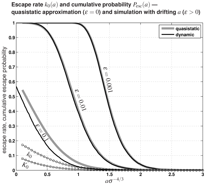
Figure 4: Escape rate $k_{0}$ from potential well for fixed $a$ (in the original parameters of (5.1)–(5.2)). The function $K_{0}(a)$ is the integral of $k_{0}$, as defined in (5.8), integrated from $a$ to $3$. The curves $\epsilon=0.1$, $\epsilon=0.01$, $\epsilon=0.001$ are the cumulative probabilities for escape from the potential well for dynamically decreasing depth of the potential well before $a$ is reached. The quantity $\epsilon$ indicates the rate of change of the potential in the unscaled parameters. For comparison the quasi-static estimate for the cumulative probability of escape is indicated using grey curves (see also Figure 5).

Figure 4 shows this escape rate $k_{0}$ as a function of $a$ as a grey curve with circles. Note that the $x$-axis corresponds to the re-scaled $a$ after transformation (5.3). An escape rate $k_{0}\approx 0.1$ at $a\sigma^{-4/3}=0.4$ means that approximately $10\%$ of the realizations cross the threshold $x_{\mathrm{th}}=-5$ to escape per unit time interval during the solution of the saddle-node normal form (5.1) with $a\sigma^{-4/3}=0.4$.

Quasi-static approximation of the cumulative escape probability

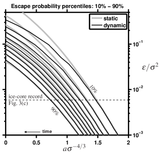
Figure 5: Percentiles of the probability of escape for dynamically varying $a$ (in black) in the original parameters of (5.1)–(5.2). For fixed $\epsilon$ the $x$%-curve shows at which $a$ $x$% of the realisations have escaped. For comparison the grey curves show the estimate obtained using the quasi-static approximation. The depth of the potential well (and, thus, $a$) decreases in time.

Using the escape rate $k_{0}(a)$ for the frozen problem ($\epsilon=0$ in (5.4)–(5.5)) we can approximate the cumulative probability $P_{\mathrm{esc}}$ of escape for a trajectory of the saddle-node normal form with drifting control parameter. If we assume that escape is irreversible and denote by $p(t)$ the probability that the trajectory has not escaped until time $t$ then we have the relation

$$p(t+h)=\left[1-(k_{0}(a(t))+O(\epsilon))h\right]p(t)$$ (5.6)

for small time steps $h>0$. The factor $1-k_{0}(a(t))h$ is the probability that the trajectory escapes during the time interval $[t,t+h]$ if we approximate the slowly changing variable $a$ by its left-end value $a(t)$ in this interval. Relation (5.6) expresses that a trajectory will not escape until time $t+h$ if it has not escaped until time $t$ and it does not escape during the interval $[t,t+h]$. Letting $h$ go to zero and ignoring the slow drift of $a$ during the time interval $[t,t+h]$ of order $O(\epsilon)$ we obtain the differential equation

$$\frac{\mathop{}\!\mathrm{d}}{\mathop{}\!\mathrm{d}t}p(t)=-k_{0}(a(t))p(t)\mbox{,}$$

which has the solution

$$p(t)=\exp\left(\int_{0}^{t}-k_{0}(a(s))\mathop{}\!\mathrm{d}s\right)$$ (5.7)

if we start with an initial distribution concentrated in the potential well ($p(0)=1$). We want to find the approximate cumulative probability $P_{\mathrm{esc}}(a)$ of escape before the control has drifted to a certain value $a$, so we substitute $a=a(0)-\epsilon t$ into expression (5.7) for $p(t)$:

$$P_{\mathrm{esc}}(a)=1-\exp\left(-K_{0}(a)/\epsilon\right)\mbox{\quad where \quad}K_{0}(a)=\int_{a}^{a(0)}k_{0}(a^{\prime})\mathop{}\!\mathrm{d}a^{\prime}\mbox{.}$$ (5.8)

This approximation (5.8) for the escape probability assumes that $\epsilon$ is small, that the escape is irreversible (which is accurate if the threshold $x_{\mathrm{th}}$ is sufficiently negative), and that $a(0)\gg 1$ (which makes $P_{\mathrm{esc}}$ nearly independent of the initial distribution of $x$).

Figure 4 shows the quasi-static approximation of the cumulative escape probability $P_{\mathrm{esc}}$ for $\epsilon=0.1$, $0.01$ and $0.001$ as grey curves. Superimposed are numerical observations of the cumulative escape probability $P_{\mathrm{esc}}$ for the normal form with drifting parameter $a$ (5.4)–(5.5) as black curves. In a simulation of (5.4)–(5.5) one can approximate the cumulative escape probability $P_{\mathrm{esc}}$ until time step $t_{n}$ with the help of a recursion for the probability $1-P_{\mathrm{esc}}$ of not escaping

$$1-P_{\mathrm{esc}}(t_{n+1})=\frac{N-N_{\mathrm{esc}}(t_{n})}{N}(1-P_{\mathrm{esc}}(t_{n}))$$

where $N_{\mathrm{esc}}(t_{n})$ is the number of realisations that escape at time step $t_{n}$ and $N$ is the overall ensemble size. We keep the overall ensemble size $N$ (of non-escaped realisations) constant by re-initialising every escaped realisation to a random non-escaped instance.

One can see that if the control parameter $a$ drifts slowly ($\epsilon\ll 1$) the cumulative escape probability increases sharply from nearly $0$ to nearly $1$ in a range of $a$ of about length $1$ (for example, between $a=1$ and $a=2$ for $\epsilon=0.001$).

Figure 5 shows the percentiles of the cumulative escape probabilities systematically for $\epsilon$ ranging between $0.001$ and $0.5$. Again, we superimpose black curves showing the percentiles of the cumulative probability observed during a simulation of the normal form with drifting control parameter (5.4)–(5.5).

We draw two conclusions from the results shown in Figure 4 and Figure 5:

1. the quasi-static approximation (5.8) of the cumulative escape probability is quantitatively accurate to order $\epsilon$. For large $\epsilon$ ($\sim 0.1$) the effect of the dynamic drifting of the control parameter delays the escape slightly. Naturally, this effect is much weaker than the delay in exchange of stability observed in slow passages through Hopf or Pitchfork bifurcations (see (Kuske, 1999; Baer et al., 1989; Su et al., 2004) for studies that quantify also the effect of noise).

2. Random disturbances make early escape probable as soon as the ratio of drift speed $\epsilon$ and variance of the disturbance $\sigma^{2}$ becomes small in the original parameters of saddle-node normal form with drift and noise (5.1)–(5.2). The percentiles in Figure 5 quantify this effect after the axes have been scaled using transformation (5.3): $\epsilon\mapsto\epsilon\sigma^{-2}$, $a\mapsto a\sigma^{-4/3}$.

Control of accuracy in stochastic simulations

The ensemble size for the numerical simulation was $N=400$, and the integration was performed with the Euler-Maruyama scheme (which of order $1$ for this problem) using stepsize $h=0.01$. Control calculations using different method parameters give results that are visually indistinguishable from Figure 4. For control we varied (one-by-one) the stepsize ($h=0.05$), the threshold for a realisation to count as escaped ($x_{\mathrm{th}}=-10$), and the ensemble size ($N=800$). We also varied the re-initialisation strategy: alternatively we chose the new position of a particle after escape according to a Gaussian distribution with mean $X_{s}=\sqrt{a}$ (the bottom of the well) and variance $\sigma^{2}/\sqrt{a}$. This would be the stationary distribution obtained for the linearisation of the re-scaled normal form (5.4) in its equilibrium $X_{s}$. This alternative re-initialisation works by construction only for $a>0$.

The Figures 4 and 5 both show either long-time limits (such as $k_{0}(a)$ in Figure 4) or cumulative quantities: $K_{0}(a)$ and $P_{\mathrm{esc}}$. These quantities can be approximated more accurately with relatively small ensemble sizes and simple ensemble integration than, for example, probability densities. The density of the escape probability is the time derivative of $P_{\mathrm{esc}}$, which would be a much “noisier” function of time (or $a$) for finite randomly drawn ensembles than $P_{\mathrm{esc}}$ unless one applies more sophisticated numerical methods and uses larger ensemble sizes (Kuske, 1999, 2000).

For large $a$ numerical simulations of the stochastic differential equation (5.4) become inefficient because escape events become extremely rare. However, this case is covered analytically by classical chemical reaction rate theory (Hänggi et al., 1990):

$$k_{0}(a)\sim\frac{2\sqrt{a}}{\pi}\exp\left(-2\sqrt{a}\right)\mbox{\ for $a\gg 1$,}$$ (5.9)

where the expression on the right-hand side contains the dominant terms of $a$ in the pre-factor and in the exponent. Thus, replacing the upper limit of integration $a(0)$ by $+\infty$ in the approximation (5.8) of $P_{\mathrm{esc}}$ gives only a small change.

5.2 Extraction of noise-induced escape probability from time series

In order to estimate if noise-induced early escape plays a role one needs to assume that the time series $z_{k}$ is generated by a system with a parameter that drifts and approaches a saddle-node bifurcation. We denote the drifting parameter by $a$ in a manner that the saddle-node bifurcation is at $a=0$ and equilibria of the deterministic system with fixed $a$ exist for $a>0$. We introduce the parameter $Z_{0}$ as the $z$-value of the equilibrium at the saddle-node parameter $a=0$. If we assume that the underlying process is subject to an additive (Gaussian) perturbation of amplitude $\sigma_{z}$ then $z_{k}$ can be written as the measurements of the system

$$\mathop{}\!\mathrm{d}z =\left[qa(t)-\frac{(z-Z_{0})^{2}}{q}+O((z-Z_{0})^{3})\right]\mathop{}\!\mathrm{d}t+\sigma_{z}\mathop{}\!\mathrm{d}W_{t}$$ (5.10)

at times $k\Delta t$. The parameter $q$ in (5.10) measures the width of the parabola $a(z)$ of equilibria of (5.10) for zero noise amplitude ($\sigma_{z}=0$) and ignoring third-order powers of $z-Z_{0}$:

$$a(z)=\frac{(z-Z_{0})^{2}}{q^{2}}\mbox{.}$$

If $q$ is negative then the stable side of the parabola is below $Z_{0}$, if $q$ is positive then the stable side is above $Z_{0}$. From the general form (5.10) of a system near a saddle-node one can obtain the normal form

$$\mathop{}\!\mathrm{d}x=\left[a(t)-x^{2}\right]\mathop{}\!\mathrm{d}t+\sigma\mathop{}\!\mathrm{d}W_{t}$$ (5.11)

by ignoring third-order powers of $z-Z_{0}$ and introducing the re-scaled variable

$$x=\frac{z-Z_{0}}{q}\mbox{.}$$

The noise amplitude scales correspondingly:

$$\sigma=\frac{\sigma_{z}}{q}\mbox{.}$$ (5.12)

We demonstrate how to extract a (crude) estimate of the state and the parameters of (5.10) from a time series $z_{k}$ as shown, for example, for the model output in Figure 3(a,b). As long as $a(t)$ is large the potential well is deep such that the Gaussian perturbation $\sigma_{z}\mathop{}\!\mathrm{d}W_{t}$ is unlikely to kick $z(t)$ out of the well of the stable equilibrium. Choosing $\Delta t$ (the time spacing of the measurements $z_{k}$) as our time unit we first revert the estimates $c_{k}$ and $\theta_{k}$ obtained from the degenerate finger-printing into estimates of the parameters $\kappa(t)$ and $\sigma(t)$ appearing in the Ornstein-Uhlenbeck process obtained from linearising (5.10) in its stable equilibrium at $q\sqrt{\smash[b]{a}}$:

$$\mathop{}\!\mathrm{d}z=-\kappa(t)z\mathop{}\!\mathrm{d}t+\sigma_{z}(t)\mathop{}\!\mathrm{d}W_{t}\mbox{.}$$

The estimates $\kappa_{k}$ for $\kappa(k\Delta t)$ and $\sigma_{k}$ for $\sigma(k\Delta t)$ are

$$\kappa_{k} =-\log c_{k}$$ (5.13)

where the estimate $$c_{k}$$ is calculated using the fitting procedure in Section 3.2 and

$$\sigma_{z,k} =\theta_{k}\sqrt{\frac{2\kappa_{k}}{(1-c_{k}^{2})}}$$ (5.14)

(see (Gillespie, 1992)) where $\theta_{k}$ is the standard deviation of the detrended time series from the AR(1) estimate. The estimate $\kappa_{k}$ is an approximation of the linear decay rate

$$\kappa(k\Delta t)=2\sqrt{a(k\Delta t)}$$ (5.15)

as long the time series $z_{k}$ is near the bottom of the potential well. Thus, we can estimate $a(k\Delta t)$ for the times $k\Delta t$ as $a_{k}$:

$$a_{k}=\frac{\kappa_{k}^{2}}{4}\mbox{.}$$

Consequently, estimates of the parameters $a$ and $\sigma_{z}$ are by-products of the AR(1) estimate to obtain $c_{k}$. The only remaining unknown quantity that one needs to convert to the normal form (5.11) is the scaling factor $q$. If we drop third-order terms of $z-Z_{0}$, fix $a$ at $a_{k}$, and consider only the deterministic part ($\sigma_{z}=0$) then the equilibrium $Z_{k}$ of (5.10) satisfies $\sqrt{\smash[b]{a_{k}}}q-Z_{k}+Z_{0}=0$, which is equivalent to

$$\frac{\kappa_{k}}{2}q+Z_{0}=Z_{k}\mbox{.}$$ (5.16)

We see that $q$ is the ratio between the slope of $\kappa_{k}/2$ (for which we have an estimate) and the slope of the equilibrium state which the time series $z_{k}$ fluctuates around. An estimate for $Z_{k}$ has also been obtained during the degenerate finger-printing procedure as the kernel-average of $z_{k}$ (also named $Z_{k}$ in Section 3.2). Thus, an estimate for $q$ is the ratio between the mean slope of $Z_{k}$ and the mean slope of $\kappa_{k}$.

In our analysis of the normal form with drift and noise we considered the case were the parameter $a$ drifts with a uniform (small) speed $\epsilon$. This is unrealistic for paleo-climate records and in models whenever the parameter $a$ is driven by the output of another subsystem, for example, if $a$ is freshwater forcing as in (Rahmstorf, 2000). In order to predict how the parameter $a$ continues to drift beyond the final sliding window we assume that the process driving $a$ is stationary. So,

$$a(t)=a(0)-\int_{0}^{t}\epsilon(s)\mathop{}\!\mathrm{d}s$$ (5.17)

where $\epsilon$ is not constant but a random variable with a stationary probability distribution. The distribution has been estimated for the period of time where $\kappa$ is available: $\epsilon_{k}$ are the increments between successive $a$ estimates:

$$\epsilon_{k}=\frac{a_{k}-a_{k+1}}{\Delta t}\mbox{.}$$

These $\epsilon_{k}$ form an empirical sample of the distribution of $\epsilon(s)$ from which we can draw to calculate $a(t)$ using (5.17) without estimating any further parameters. If the mean of $\epsilon$ exists and is bigger than zero then $a(t)$ will reach $0$ almost surely, resulting in a probability distribution

$$P_{a}(t)=1-P\left(a(s)>0\phantom{|_{|}}\mbox{\ for all $s<t$}\right)\mbox{,}$$

which is the probability that the random variable $a$ reaches its critical value $a=0$ before time $t$. The probability $P_{\mathrm{esc}}(t)$ of a trajectory escaping before time $t$ can now be estimated using a direct numerical simulation of

$$\begin{split}\mathop{}\!\mathrm{d}x&=\left[a-x^{2}\right]\mathop{}\!\mathrm{d}t+\sigma\mathop{}\!\mathrm{d}W_{t}\\ \mathop{}\!\mathrm{d}a&=-\epsilon(t)\mathop{}\!\mathrm{d}t\mbox{.}\end{split}$$

Alternatively, if the mean of $\epsilon$ is sufficiently small one can use the quasi-static approximation

$$P_{\mathrm{esc}}(t)=1-E\left[\exp\left(\int_{0}^{t}k_{0}(a(s))\mathop{}\!\mathrm{d}s\right)\right]$$

where the escape rate $k_{0}(a)$ (which exists only for positive $a$) is given in Figure 4 and $E[x]$ is the mean of the random variable $x$.

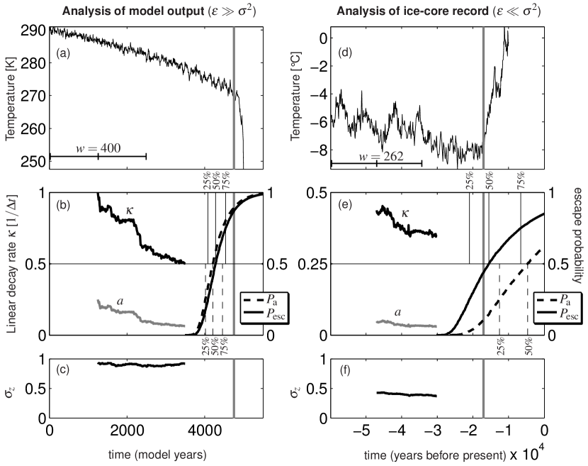
Figure 6: Prediction of saddle-node bifurcation and early escape for two time series shown in (Dakos et al., 2008). Diagram (a) shows the stochastic model output also shown in Figure 3(a). All quantities have been obtained only from data prior to the cut-off time indicated by the grey vertical line in diagram (a). Diagram (b) shows the linear decay rate $\kappa_{k}$ (as extracted by degenerate finger-printing with window size $w$, compare to Figure 3(b)) and the corresponding normal form parameter $a$. It also contains the cumulative probability functions for reaching the critical value $a=0$ and for escape, $P_{a}$ and $P_{\mathrm{esc}}$ on the right axis. The graph in diagram (c) is the estimated noise amplitude $\sigma$ extracted from the time series. The diagrams (d-f) discuss the time series shown in Figure 3(c), which is a snapshot from the paleo-climate record of Petit et al. (1999) at the end of the last glaciation using the identical procedure to the one applied to the time series in diagram (a).

Parameter	Model output Figure 6(a–c)	Ice-core record Figure 6(d–f)
mean $\epsilon$	$2.2\times 10^{-4}$	$5.2\times 10^{-6}$
stdev $\epsilon$	$1.1\times 10^{-3}$	$5.9\times 10^{-5}$
$q$	$621$	$13.5$
$\sigma$	$1.4\times 10^{-3}$	$3.0\times 10^{-2}$
mean $\epsilon\sigma^{-2}$	$105$	$5.9\times 10^{-3}$

Table 1: Numerical values of estimates of parameters that are not visible in Figure 6.

Figure 6(b) and (c) show the quantities $\kappa_{k}$, $a_{k}$ and $\sigma_{z,k}$ for the time series $z_{k}$ of the stochastic model output in Figure 6(a) (the same series $z_{k}$ as in Figure 3(a)). Figure 6(b) also shows the cumulative probability function $P_{a}(t)$ for $a$ crossing the critical value $0$ before $t$ (dashed curve) and its quartiles (dashed threshold lines), and the probability $P_{\mathrm{esc}}(t)$ for escape before time $t$ (solid curve) and its quartiles (solid threshold lines). The threshold for a trajectory counting as escaped was set at $x_{\mathrm{th}}=-5$. Table 1 lists the values of $q$ as determined by relation (5.16) and $\sigma=\sigma_{z}/q$. Also, the table lists the empirical mean value of the random variable $\epsilon$ and its empirical standard deviation (the distribution of $\epsilon$ is only moderately skewed). The mean of $\epsilon/\sigma^{2}$ indicates if the parameter drift is rapid or slow in rescaled normal form coordinates. Figure 6(e) and (f) show the quantities $\kappa$, $a$, $P_{\mathrm{esc}}$, $P_{a}$ and $\sigma_{z}$ for the ice-core record in Figure 6(d) (the same series $z_{k}$ as in Figure 3(c))

We observe that the parameter drift in the model output (see Figure 6(b)) is fast compared to the noise level such that early escape plays no role. Table 1 also shows that the ratio between drift and variance is large, which confirms the visual impression that drift dominates the noise. The probability distribution for escape is even shifted to the right such that trajectories are expected to escape later than the drifting system parameter $a$ reaches its critical value.

We note that the actual escape of the observed instance from Figure 6(a) occurs relatively late (at the $90\%$ percentile). This shifts down (to below $75\%$) for shorter sliding windows in the degenerate finger-printing procedure. Both probability distributions are relatively symmetric and concentrated in a range of approximately $1\,000$ model years.

In contrast, the time series of the ice-core record, shown in Figure 6(d), has a slowly drifting parameter compared to the noise level (note that one cannot be certain that the underlying mechanism for the apparent tipping is indeed a passage through a saddle-node). Consequently, trajectories of the estimated saddle-node normal form system escape significantly earlier than $a$ reaches its critical value: the cumulative probability $P_{\mathrm{esc}}$ is shifted to the left of $P_{a}$. For example, the median ($50\%$) time for escape is $1.1\times 10^{4}$ years before the median time for reaching the critical value $a=0$. We notice that both distributions, $P_{a}$ and $P_{\mathrm{esc}}$ are highly skewed, having a long tail at the right end. This makes the expected escape time (mean escape time) as a point estimate sensitive to small perturbations such as measurement uncertainty or a different choice of method parameters in the degenerate finger-printing procedure whereas the median times are comparatively robust. A systematic analysis, including the dependence on the cut-off time (the grey vertical line in all panels of Figure 6), is a topic for future work.

6 Conclusion

Methods to identify incipient climate tipping using time series analysis have recently been developed by Held and Kleinen (2004) and Livina and Lenton (2007). These methods have been tested on model outputs and paleo-climate data by Livina and Lenton (2007) and Dakos et al. (2008). Time series analysis should be seen as a complement to the huge modelling efforts that are invested into the analysis and prediction of climate changes. While Dakos et al. (2008) could demonstrate that the characteristic quantity extracted from the time series, the propagator, indeed increases (as it should according to bifurcation theory) using this quantity for prediction is much more challenging. The extraction of the propagator from a time series makes assumptions that are, for archaeological records, difficult to check: for example, separation of time scales between parameter drift, decay of critical mode and decay of stable modes, or the nearly constant-speed approach of the underlying control parameter toward its critical value.

We studied another source of uncertainty, which exists even if the underlying deterministic dynamics is drifting with constant speed close to a saddle-node bifurcation and the estimated linear decay rate is accurate. Namely, the escape of the dynamics from the potential well around the stable equilibrium can be either premature or delayed, depending on the ratio between parameter drift speed and the amplitude of the random disturbances. We derived an approximate (semi-analytic) formula that is valid in the quasi-static limit (that is, the parameter drifts sufficiently slowly compared to the noise amplitude). We found that the early escape effect vanishes if the drift is more rapid (drift speed $\epsilon\approx 0.3$ in normal form scaling).

We also demonstrated how one can estimate this effect from time series data, using what we might call a ‘fold for incipient tipping’ method (FIT). This was tested for two examples, the output of a stochastic model (a case of rapid drift) and an ice-core record (a case of slow drift, or large noise amplitude). We plan to study the consistency of the proposed escape prediction for time series more systematically in the future. This should be done by generating time series instances from saddle-node normal forms with drifting parameter and noise, predicting escape distributions from these time series, and then comparing the predictions to the original distributions shown in Figure 5.

Our estimates for early escape from a potential well are all stated in probabilistic terms, which is appropriate if one treats the disturbances as random. Normal form based estimates such as ours may also be useful when studying tipping in climate models because running simulations for large ensembles of realizations in sophisticated climate models is expensive. If the modelled scenario is close to tipping and deterministic calculations reveal the presence of a saddle-node bifurcation then the diagrams in Figure 4 and Figure 5 help to give estimates for the escape probability depending on the speed of parameter drift and the amplitude of the disturbances.

Finally, we note that our scenario corresponds to the escape from a potential well of an overdamped particle (this appears to be the relevant case, for example, in ocean circulation models, see (Dijkstra et al., 2004)). The weakly damped case,

$$\frac{\mathop{}\!\mathrm{d}^{2}x}{\mathop{}\!\mathrm{d}t^{2}}+\gamma\frac{\mathop{}\!\mathrm{d}x}{\mathop{}\!\mathrm{d}t}=-U(x)+\sigma\xi(t)\mbox{,}$$

where $\gamma$ is a small coefficient determining the amount of damping ($0<\gamma\ll 1$), $U$ is the potential and $\xi$ is the disturbance (for example, a random Gaussian noise), has also been covered by reaction rate theory (the classical theory treats the case where the noise amplitude $\sigma$ is much smaller than the potential barrier, see (Hänggi et al., 1990) for a review).

References

- Alley et al. (2003) Alley, R. B., Marotzke, J., Nordhaus, W. D., Overpeck, J. T., Peteet, D. M., Pielke, R. A., Pierrehumbert, R. T., Rhines, P. B., Stocker, T. F., Talley, L. D., and Wallace, J. M. (2003). Abrupt climate change. Science, 299(5615), 2005–2010.
- Baer et al. (1989) Baer, S. M., Erneux, T., and Rinzel, J. (1989). The Slow Passage Through a Hopf Bifurcation: Delay, Memory Effects, and Resonance. SIAM Journal on Applied Mathematics, 49(1), 55 – 71.
- Copenhagen (2009) Copenhagen (2009). United Nations Climate Change Conference, Dec 7-18, 2009. Copenhagen.
- Corsi and Taranta (2007) Corsi, S. and Taranto, G. N. (2007). Voltage instability - the different shapes of the nose. In iREP Symposium- Bulk Power System Dynamics and Control - VII, Revitalizing Operational Reliability, Charleston, SC. IEEE.
- Dakos et al. (2008) Dakos, V., Scheffer, M., van Nes, E. H., Brovkin, V., Petoukhov, V., and Held, H. (2008). Slowing down as an early warning signal for abrupt climate change. Proceedings of the National Academy of Sciences of the United States of America, 105(38), 14308–14312.
- Dijkstra et al. (2004) Dijkstra, H. A., te Raa, L., and Weijer, W. (2004). A systematic approach to determine thresholds of the ocean’s thermohaline circulation. Tellus. Series A, Dynamic meteorology and oceanography, 56(4), 362–370.
- Fischer and Imkeller (2006) Fischer, M. and Imkeller, P. (2006). Noise-Induced Resonance in Bistable Systems Caused by Delay Feedback. Stochastic Analysis and Applications, 24(1), 135–194.
- Fraedrich (1978) Fraedrich, K. (1978). Structural and stochastic analysis of a zero-dimensional climate system. Quarterly Journal of the Royal Meteorological Society, 104(440), 461–474.
- Gillespie (1992) Gillespie, D. T. (1992). Markov Processes: An Introduction for physical Scientists. Academic Press, New York.
- Hänggi et al. (1990) Hänggi, P., Talkner, P., and Borkovec, M. (1990). Reaction-rate theory: fifty years after Kramers. Reviews of Modern Physics, 62(2), 251–341.
- Held and Kleinen (2004) Held, H. and Kleinen, T. (2004). Detection of climate system bifurcations by degenerate fingerprinting. Geophysical Research Letters, 31(23), L23207.
- Houghton (2004) Houghton, J. T. (2004). Global warming: the complete briefing. Cambridge University Press, Cambridge, UK.
- IPCC (2007) IPCC (2007). Climate Change 2007, Contribution of Working Groups I-III to the Fourth Assessment Report of the Intergovernmental Panel on Climate Change, I The Physical Science Basis, II Impacts, Adaptation and Vulnerability, III Mitigation of Climate Change. Cambridge University Press, Cambridge, UK.
- Kuske (1999) Kuske, R. (1999). Probability Densities for Noisy Delay Bifurcations. Journal of Statistical Physics, 96(3), 797–816.
- Kuske (2000) Kuske, R. (2000). Gradient-Particle Solutions of Fokker–Planck Equations for Noisy Delay Bifurcations. SIAM Journal on Scientific Computing, 22(1), 351–367.
- Lenton et al. (2008) Lenton, T. M., Held, H., Kriegler, E., Hall, J. W., Lucht, W., Rahmstorf, S., and Schellnhuber, H. J. (2008). Tipping elements in the Earth’s climate system. Proceedings of the National Academy of Sciences of the United States of America, 105(6), 1786–1793.
- Livina and Lenton (2007) Livina, V. N. and Lenton, T. M. (2007). A modified method for detecting incipient bifurcations in a dynamical system. Geophysical Research Letters, 34(3), L03712.
- Lockwood (2001) Lockwood, J. (2001). Abrupt and sudden climatic transitions and fluctuations: a review. International Journal of Climatology, 21(9), 1153–1179.
- Malakhov and Pankratov (1996) Malakhov, A. and Pankratov, A. L. (1996). Influence of thermal fluctuations on time characteristics of a single Josephson element with high damping exact solution. Physica C: Superconductivity, 269(1-2), 46–54.
- National Research Council (2002) National Research Council (2002). Abrupt Climate Change: Inevitable Surprises. Natl Acad Press, Washington, DC.
- Petit et al. (1999) Petit, J. R., Jouzel, J., Raynaud, D., Barkov, N. I., Barnola, J.-M., Basile, I., Bender, M., Chappellaz, J., Davis, M., Delaygue, G., Delmotte, M., Kotlyakov, V. M., Legrand, M., Lipenkov, V. Y., Lorius, C., Pépin, L., Ritz, C., Saltzman, E., and Stievenard, M. (1999). Climate and atmospheric history of the past 420,000 years from the Vostok ice core, Antarctica. Nature, 399(6735), 429–436.
- Rahmstorf (2000) Rahmstorf, S. (2000). The Thermohaline Ocean Circulation: A System with Dangerous Thresholds? Climatic Change, 46(3), 247–256.
- Rahmstorf (2001) Rahmstorf, S. (2001). Abrupt Climate Change. In J. Steele, S. Thorpe, and K. Turekian, editors, Encyclopaedia of Ocean Sciences, pages 1–6. Academic Press, London, UK.
- Rial et al. (2004) Rial, J. A., Pielke, R. A., Beniston, M., Claussen, M., Canadell, J., Cox, P., Held, H., de Noblet-Ducoudré, N., Prinn, R., Reynolds, J. F., and Salas, J. D. (2004). Nonlinearities, Feedbacks and Critical Thresholds within the Earth’s Climate System. Climatic Change, 65(1/2), 11–38.
- Scheffer (2009) Scheffer, M. (2009). Critical Transitions in Nature and Society. Princeton University Press, Princeton, USA.
- Su et al. (2004) Su, J., Rubin, J., and Terman, D. (2004). Effects of noise on elliptic bursters. Nonlinearity, 17(1), 133–157.
- Thompson and Sieber (2010) Thompson, J. M. T. and Sieber, J. (2010). Predicting Climate Tipping Points. In B. Launder and J. M. T. Thompson, editors, Geo-Engineering Climate Change: Environmental necessity or Pandora’s Box?, chapter 3, pages 50–83. Cambridge University Press, Cambridge, UK.
- Thompson and Stewart (2002) Thompson, J. M. T. and Stewart, H. B. (2002). Nonlinear dynamics and chaos. Wiley, Chichester, UK, 2 edition.
- Thompson et al. (1994) Thompson, J. M. T., Stewart, H. B., and Ueda, Y. (1994). Safe, explosive, and dangerous bifurcations in dissipative dynamical systems. Physical Review E, 49(2), 1019–1027.