Low Complexity Linear Programming Decoding of Nonbinary Linear Codes

Abstract

Linear Programming (LP) decoding of Low-Density Parity-Check (LDPC) codes has attracted much attention in the research community in the past few years. The aim of LP decoding is to develop an algorithm which has error-correcting performance similar to that of the Sum-Product (SP) decoding algorithm, while at the same time it should be amenable to mathematical analysis. The LP decoding algorithm has been derived for both binary and nonbinary decoding frameworks. However, the most important problem with LP decoding for both binary and nonbinary linear codes is that the complexity of standard LP solvers such as the simplex algorithm remain prohibitively large for codes of moderate to large block length. To address this problem, Vontobel et al. proposed a low complexity LP decoding algorithm for binary linear codes which has complexity linear in the block length. In this paper, we extend the latter work and propose a low-complexity LP decoding algorithm for nonbinary linear codes. We use the LP formulation for the nonbinary codes as a basis and derive a pair of primal-dual LP formulations. The dual LP is then used to develop the low-complexity LP decoding algorithm for nonbinary linear codes. The complexity of the proposed algorithm is linear in the block length and is limited mainly by the maximum check node degree. As a proof of concept, we also present a simulation result for a $[80,48]$ LDPC code defined over $\mathbb{Z}_{4}$ using quaternary phase-shift keying over the AWGN channel, and we show that the error-correcting performance of the proposed LP decoding algorithm is similar to that of the standard LP decoding using the simplex solver.

I INTRODUCTION

Low-Density Parity-Check (LDPC) codes belong to the class of capacity achieving codes. They were introduced in the early 1960s by Gallager [1] but attracted the attention of the research community only after they were rediscovered by MacKay et al. in the late 1990s [2]. LDPC codes are generally decoded by the belief propagation algorithm (also known as the Sum-Product (SP) algorithm) which has time complexity linear in the block length. However, binary LDPC codes suffer from an error floor effect in the high SNR region. Some progress has been made in the direction of finite length analysis of LDPC codes and concepts such as graph-cover pseudocodewords, trapping sets, stopping sets etc. were introduced and investigated to understand the behavior of the SP algorithm. Nevertheless, finite length analysis of LDPC codes under the SP algorithm is a difficult task and it is still difficult to predict error floor behavior for a particular code.

The main focus of research in the area of LDPC codes has been on binary LDPC codes. However, it is desirable to use nonbinary LDPC codes in many applications where bandwidth efficient higher order (i.e. nonbinary) modulation schemes are used. Nonbinary LDPC codes are also considered for storage applications [12]. Nonbinary LDPC codes and the corresponding nonbinary SP algorithm were investigated by Davey and MacKay in [3] and since then many code construction methods and optimized nonbinary SP algorithms have been proposed. However, finite length analysis of nonbinary LDPC codes under the nonbinary SP algorithm is also difficult and very few attempts (e.g. [14]) have been made in this direction.

An alternative decoding algorithm for binary LDPC codes, known as Linear Programming (LP) decoding, was proposed by Feldman et al. [8]. In LP decoding, the ML decoding problem is modeled as an Integer Programming (IP) problem which is then relaxed to obtain the corresponding LP problem. This LP problem is solved with the help of standard LP solvers such as simplex. Compared to SP decoding, LP decoding relies on the well-studied mathematical theory of LP. Hence, the LP decoding algorithm is better suited to mathematical analysis and it is possible to make statements about its complexity and convergence, as well as to place bounds on its error-correcting-performance etc. However, the worst-case time complexity of the simplex solver is known to be exponential in the number of variables, which limits the use of LP decoding algorithms to codes of small block length. To overcome the complexity problem, in [9] Vontobel et al. used techniques from LP and coding theory to derive a low-complexity LP decoding algorithm for approximate LP decoding. The complexity of this latter LP decoding algorithm is linear in the block length and similar to that of the SP algorithm. A similar algorithm for more general graphical models is proposed in [10]. An extension of low-complexity LP decoding algorithm of [9] was proposed and studied in [13].

In [11], the LP decoding algorithm for binary linear codes was extended to the case of nonbinary linear codes. The nonbinary LP decoding algorithm of [11] also relies on the simplex LP solver and hence its complexity is prohibitively large for moderate and large block length codes. In this paper we extend the work of [9] and propose a low-complexity LP decoding algorithm for nonbinary linear codes. We use the LP formulation of nonbinary linear codes proposed in [11] to develop an equivalent primal LP formulation. Then using the the techniques introduced in [5, 6], the corresponding dual LP is derived which in turn is used to develop an update equation for the low-complexity LP decoding algorithm. This paper follows the development of the low-complexity LP decoder for binary LDPC codes proposed in [9]. However, there are three main points in which it differs from the work in [9]; first, the derivation of the primal-dual LP formulations for nonbinary linear codes; second, the update equation for the low-complexity LP decoding of nonbinary codes; and third, the decision rule required to obtain an estimate of the symbols after the algorithm terminates.

The rest of the paper is structured as follows. We begin with some notation and background information in Section II. The primal LP is developed in Section III and the corresponding dual LP is given in Section IV. The notion of “local function” is given in Section V. Section VI presents the low-complexity LP decoding algorithm for nonbinary linear codes. Simulation results are presented and discussed in Section VII. Conclusions are given in Section VIII, along with future directions for this research.

II Notation and Background

Let $\Re$ be a finite ring with $q$ elements where $0$ denotes the additive identity, and let $\Re^{-}=\Re\setminus\{0\}$. Let $\mathcal{C}$ be a linear code of length $n$ over the ring $\Re$, defined by

$$\mathcal{C}=\{{\boldsymbol{c}}\in\Re^{n}:{\boldsymbol{c}}\mathcal{H}^{T}={\boldsymbol{0}}\}$$ (1)

where $\mathcal{H}$ is a $m\times n$ parity-check matrix with entries from $\Re$. The rate of code $\mathcal{C}$ is given by $R(\mathcal{C})=\log_{q}(|\mathcal{C}|)/n$. Hence, the code $\mathcal{C}$ can be referred as an $[n,\log_{q}(|\mathcal{C}|)]$ linear code over $\Re$.

The set $\mathcal{J}=\{1,\ldots,m\}$ denotes row indices and the set $\mathcal{I}=\{1,\ldots,n\}$ denotes column indices of $\mathcal{H}$. We use $\mathcal{H}_{j}$ for the $j$-th row of $\mathcal{H}$ and $\mathcal{H}^{i}$ for the $i$-th column of $\mathcal{H}$. supp$({\boldsymbol{c}})$ denotes the support of the vector ${\boldsymbol{c}}$. For each $j\in\mathcal{J}$, let $\mathcal{I}_{j}=\mbox{supp}(\mathcal{H}_{j})$ and for each $i\in\mathcal{I}$, let $\mathcal{J}_{i}=\mbox{supp}(\mathcal{H}^{i})$. Also let $d_{j}=|\mathcal{I}_{j}|$ and $d=\max_{j\in\mathcal{J}}\{d_{j}\}$. We define set $\mathcal{E}=\{(i,j)\in\mathcal{I}\times\mathcal{J}\;:\;j\in\mathcal{J},i\in\mathcal{I}_{j}\}=\{(i,j)\in\mathcal{I}\times\mathcal{J}\;:\;i\in\mathcal{I},j\in\mathcal{J}_{i}\}$. Moreover for each $j\in\mathcal{J}$ we define the local Single Parity Check (SPC) code

$$\mathcal{C}_{j}=\left\{(b_{i})_{i\in\mathcal{I}_{j}}:\sum_{i\in\mathcal{I}_{j}}b_{i}\cdot\mathcal{H}_{j,i}=0\right\}$$

For each $i\in\mathcal{I}$, we denote by $\mathcal{A}_{i}\subseteq\Re^{|\{0\}\cup\mathcal{J}_{i}|}$ the repetition code of the appropriate length and indexing. In addition, we use the following notation introduced in [9]: for a statement $A$ we have $\llbracket$A$\rrbracket=0$ if statement $A$ is true and $\llbracket A\rrbracket=+\infty$ otherwise. Here $\llbracket A\rrbracket=-\log[A]$ and $[A]$ is Iverson’s convection i.e. we have $[A]=1$ if $A$ is true and $[A]=0$ otherwise. Please note that where $A$ indicates the value of a variable, Iverson’s convention can also be interpreted as the Kronecker delta function. We define the following mapping as in [11],

$$\xi:\Re\rightarrow\{0,1\}^{q-1}\subset\mathbb{R}^{q-1}$$

by

$$\xi(\alpha)={\boldsymbol{x}}=(x^{(\rho)})_{\rho\in\Re^{-}}$$

such that, for each $\rho\in\Re^{-}$

$$x^{(\rho)}=\left\{\begin{array}[]{l l}1,&\;\text{if}\;\rho=\alpha\\ 0,&\;\text{otherwise}\\ \end{array}\right.$$

Building on this we define

$$\Xi:\underset{t\in\mathbb{Z}^{+}}{\cup}\Re^{t}\rightarrow\underset{t\in\mathbb{Z}^{+}}{\cup}\{0,1\}^{(q-1)t}\subset\underset{t\in\mathbb{Z}^{+}}{\cup}\mathbb{R}^{(q-1)t}\;,$$

according to

$$\Xi({\boldsymbol{c}})=(\xi(c_{1}),\dots,\xi(c_{t})),\quad\forall{\boldsymbol{c}}\in\Re^{t},t\in\mathbb{Z}^{+}\;.$$

For $\kappa\in\mathbb{R},\kappa>0$, we define the function

$${{\psi}}(x)=e^{\kappa x},$$

and its inverse

$${{\psi}}^{-1}(x)=\frac{1}{\kappa}\log(x).$$

For vectors ${\boldsymbol{f}}\in\mathbb{R}^{(q-1)n}$ we use the notation

$${\boldsymbol{f}}=({\boldsymbol{f}}_{1}\;|\;{\boldsymbol{f}}_{2}\;|\;\cdots\;|\;{\boldsymbol{f}}_{n})\quad\text{where}\quad\forall i\in\mathcal{I},{\boldsymbol{f}}_{i}=(f_{i}^{(\alpha)})_{\alpha\in\Re^{-}}$$

We also define the inverse of $\Xi$ as

$$\Xi^{-1}({\boldsymbol{f}})=(\xi^{-1}({\boldsymbol{f}}_{1}),\xi^{-1}({\boldsymbol{f}}_{2}),\cdots,\xi^{-1}({\boldsymbol{f}}_{n})).$$

Note that the inverse of $\Xi$ is well defined for any ${\boldsymbol{f}}\in\mathbb{R}^{(q-1)n}$ where each component ${\boldsymbol{f}}_{i}$, $i\in\mathcal{I}$, has entries from $\{0,1\}$ with sum at most $1$. We assume transmission over a $q$-ary input memoryless channel and also assume a corrupted codeword ${\boldsymbol{y}}=(y_{1},y_{2},\cdots,y_{n})\in\Sigma^{n}$ has been received. Here, the channel output symbols are denoted by $\Sigma$. Based on this, we define a function ${\boldsymbol{\lambda}}:\Sigma\rightarrow(\mathbb{R}\cup\{\pm\infty\})^{q-1}$ by

$${\boldsymbol{\lambda}}=(\lambda^{(\alpha)})_{\alpha\in\Re^{-}}$$

where, for each $y\in\Sigma$, $\alpha\in\Re^{-}$,

$$\lambda^{(\alpha)}(y)=\log\left(\frac{p(y|0)}{p(y|\alpha)}\right)\;.$$

Here $p(y|c)$ denotes the channel output probability (density) conditioned on the channel input. Based on this, we also define

$${\boldsymbol{\Lambda}}({\boldsymbol{y}})=({\boldsymbol{\lambda}}(y_{1})\;|\;{\boldsymbol{\lambda}}(y_{2})\;|\cdots|\;{\boldsymbol{\lambda}}(y_{n}))\;.$$

We will use Forney-style factor graphs (FFGs), also known as Normal graphs [4] to represent the linear programs introduced in this paper. An FFG is a diagram that represents the factorization of a function of several variables. For more information on FFGs the reader is referred to [4, 5, 7].

III The Primal Linear Program

In [11] the authors presented the following linear program to decode nonbinary linear codes:

NBLPD (Polytope $\mathcal{Q}_{f}$):

min. $$\quad{\boldsymbol{\Lambda}}({\boldsymbol{y}}){\boldsymbol{f}}^{T}$$

Subj. to

$$f_{i}^{(\alpha)} =\sum_{\underset{b_{i}=\alpha}{{\boldsymbol{b}}\in\mathcal{C}_{j}}}w_{j,{\boldsymbol{b}}} \forall j\in\mathcal{J},\;\forall i\in\mathcal{I}_{j},\;\forall\alpha\in\Re^{-}$$

$$w_{j,{\boldsymbol{b}}} \geq 0 \forall j\in\mathcal{J},\forall{\boldsymbol{b}}\in\mathcal{C}_{j},$$

$$\sum_{{\boldsymbol{b}}\in\mathcal{C}_{j}}w_{j,{\boldsymbol{b}}} =1 \forall j\in\mathcal{J}.$$

We denote the polytope represented by the constraints of NBLPD as $\mathcal{Q}_{f}$. Two alternative polytope representations are also given in [11], which are both equivalent to NBLPD. It also possible to reformulate the constraints of NBLPD with additional auxiliary variables. However, to develop a low-complexity LP decoding algorithm for NBLPD, we use the approach of [9] and reformulate NBLPD so that the new LP formulation can be directly represented by an FFG:

PNBLPD (Polytope $\mathcal{Q}_{p}$):

min. $$\quad{\boldsymbol{\Lambda}}({\boldsymbol{y}}){\boldsymbol{f}}^{T}$$

Subj. to

$${\boldsymbol{{f}}}_{i} ={\boldsymbol{u}}_{i,0} ( i\in\mathcal{I}),$$

$${\boldsymbol{u}}_{i,j} ={\boldsymbol{v}}_{j,i} ( (i,j)\in\mathcal{E}),$$

$$\sum_{{\boldsymbol{a}}\in\mathcal{A}_{i}}\gamma_{i,{\boldsymbol{a}}}\;\Xi({\boldsymbol{a}}) ={\boldsymbol{u}}_{i} ( i\in\mathcal{I}),$$

$$\sum_{{\boldsymbol{b}}\in\mathcal{C}_{j}}\beta_{j,{\boldsymbol{b}}}\;\Xi({\boldsymbol{b}}) ={\boldsymbol{v}}_{j} ( j\in\mathcal{J}),$$

$$\gamma_{i,{\boldsymbol{a}}} \geq 0 ( i\in\mathcal{I},{\boldsymbol{a}}\in\mathcal{A}_{i}),$$

$$\beta_{j,{\boldsymbol{b}}} \geq 0 ( j\in\mathcal{J},{\boldsymbol{b}}\in\mathcal{C}_{j}),$$

$$\sum_{{\boldsymbol{a}}\in\mathcal{A}_{i}}\gamma_{i,{\boldsymbol{a}}} =1 ( i\in\mathcal{I}),$$

$$\sum_{{\boldsymbol{b}}\in\mathcal{C}_{j}}\beta_{j,{\boldsymbol{b}}} =1 ( j\in\mathcal{J}).$$

Here ${\boldsymbol{u}}_{i,j}=(u_{i,j}^{(\alpha)})_{\alpha\in\Re^{-}}$ and ${\boldsymbol{v}}_{j,i}=(v_{j,i}^{(\alpha)})_{\alpha\in\Re^{-}}$ for all $i\in\mathcal{I}$, $j\in\mathcal{J}_{i}\cup\{0\}$; also for $i\in\mathcal{I}$, ${\boldsymbol{u}}_{i}=({\boldsymbol{u}}_{i,j})_{j\in\mathcal{J}_{i}\cup\{0\}}$ and for $j\in\mathcal{J}$, ${\boldsymbol{v}}_{j}=({\boldsymbol{v}}_{j,i})_{i\in\mathcal{I}_{j}}$. We denote the polytope represented by the constraints of PNBLPD by $\mathcal{Q}_{p}$. It is important to note that along with the convex hull of the single parity-check code, PNBLPD also explicitly models the convex hull of the repetition code. The constraints of NBLPD and PNBLPD appear to be quite different due to the different notations. However, the projection of each polytope onto the variables denoted by ${\boldsymbol{f}}$ is the same in both cases, and therefore the LPs are equivalent from the point of view of decoding. The proof of their equivalence is given in Theorem III.1.

Theorem III.1

Polytopes $\mathcal{Q}_{f}$ and $\mathcal{Q}_{p}$ are equivalent from an LP decoding perspective, i.e. for every $({\boldsymbol{f}},{\boldsymbol{\gamma}},{\boldsymbol{\beta}})\in\mathcal{Q}_{p}$ there exists ${\boldsymbol{w}}$ such that $({\boldsymbol{f}},{\boldsymbol{w}})\in\mathcal{Q}_{f}$ and conversely, for every $({\boldsymbol{f}},{\boldsymbol{w}})\in\mathcal{Q}_{f}$ there exist ${\boldsymbol{\gamma}},{\boldsymbol{\beta}}$ such that $({\boldsymbol{f}},{\boldsymbol{\gamma}},{\boldsymbol{\beta}})\in\mathcal{Q}_{p}$.

Proof:

Suppose we have $({\boldsymbol{f}},{\boldsymbol{\gamma}},{\boldsymbol{\beta}})\in\mathcal{Q}_{p}$ and we define

$$w_{j,{\boldsymbol{b}}}=\beta_{j,{\boldsymbol{b}}},\quad\forall{\boldsymbol{b}}\in\mathcal{C}_{j},\forall j\in\mathcal{J}\;.$$ (3)

The final two constraints of NBLPD are obviously fulfilled. From PNBLPD, the following holds for $({\boldsymbol{f}},{\boldsymbol{\gamma}},{\boldsymbol{\beta}})\in\mathcal{Q}_{p}$:

$${\boldsymbol{v}}_{j} =\sum_{{\boldsymbol{b}}\in\mathcal{C}_{j}}\beta_{j,{\boldsymbol{b}}}\;\Xi({\boldsymbol{b}}), \forall j\in\mathcal{J},$$

$$\Rightarrow{\boldsymbol{v}}_{j,i} =\sum_{{\boldsymbol{b}}\in\mathcal{C}_{j}}\beta_{j,{\boldsymbol{b}}}\;\xi({\boldsymbol{b}}_{i}), \forall i\in\mathcal{J}_{i},\forall j\in\mathcal{J},$$

This yields

$${v}_{j,i}^{(\alpha)} =u_{i,j}^{(\alpha)}=\sum_{\underset{{\boldsymbol{b}}_{i}=\alpha}{{\boldsymbol{b}}\in\mathcal{C}_{j}}}\beta_{j,{\boldsymbol{b}}}, \forall \alpha\in\Re^{-},\forall i\in\mathcal{I}_{j},\forall j\in\mathcal{J}.$$ (4)

From the third constraint of PNBLPD, and noting that $\mathcal{A}_{i}$ is a repetition code for each $i\in\mathcal{I}$, we have $u_{i,0}^{(\alpha)}=u_{i,j}^{(\alpha)},\forall\alpha\in\Re^{-},j\in\mathcal{J}_{i}$. With this and equation (4) we obtain the following,

$$\Rightarrow u_{i,j}^{(\alpha)} =u_{i,0}^{(\alpha)}=\sum_{{\boldsymbol{b}}\in\mathcal{C}_{j},{\boldsymbol{b}}_{i}=\alpha}\beta_{j,{\boldsymbol{b}}}$$

$$\Rightarrow f_{i}^{(\alpha)} =\sum_{\underset{{\boldsymbol{b}}_{i}=\alpha}{{\boldsymbol{b}}\in\mathcal{C}_{j}}}w_{j,{\boldsymbol{b}}},\quad\forall\alpha\in\Re^{-},\forall i\in\mathcal{I}_{j},\forall j\in\mathcal{J}.$$ (5)

This proves the first constraint of NBLPD and hence $({\boldsymbol{f}},{\boldsymbol{w}})\in\mathcal{Q}_{f}$.

The converse part of the theorem statement can be proved in a similar manner; the details are omitted. Since for a given vector ${\boldsymbol{f}}$, the objective functions in both formulations always have the same value, the decoding performance of NBLPD and PNBLPD are identical. ∎

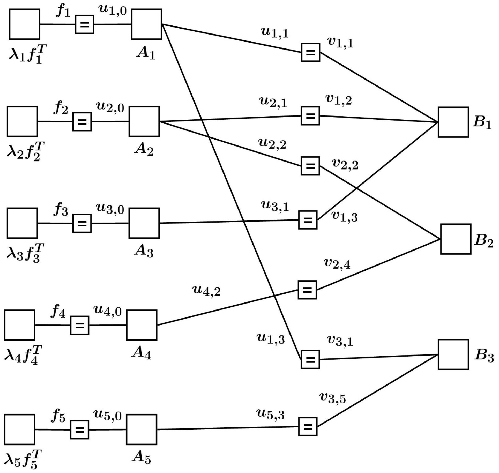
Figure 1: FFG which represents the augmented cost function of equation (6) for the example $(5,2)$ binary code.

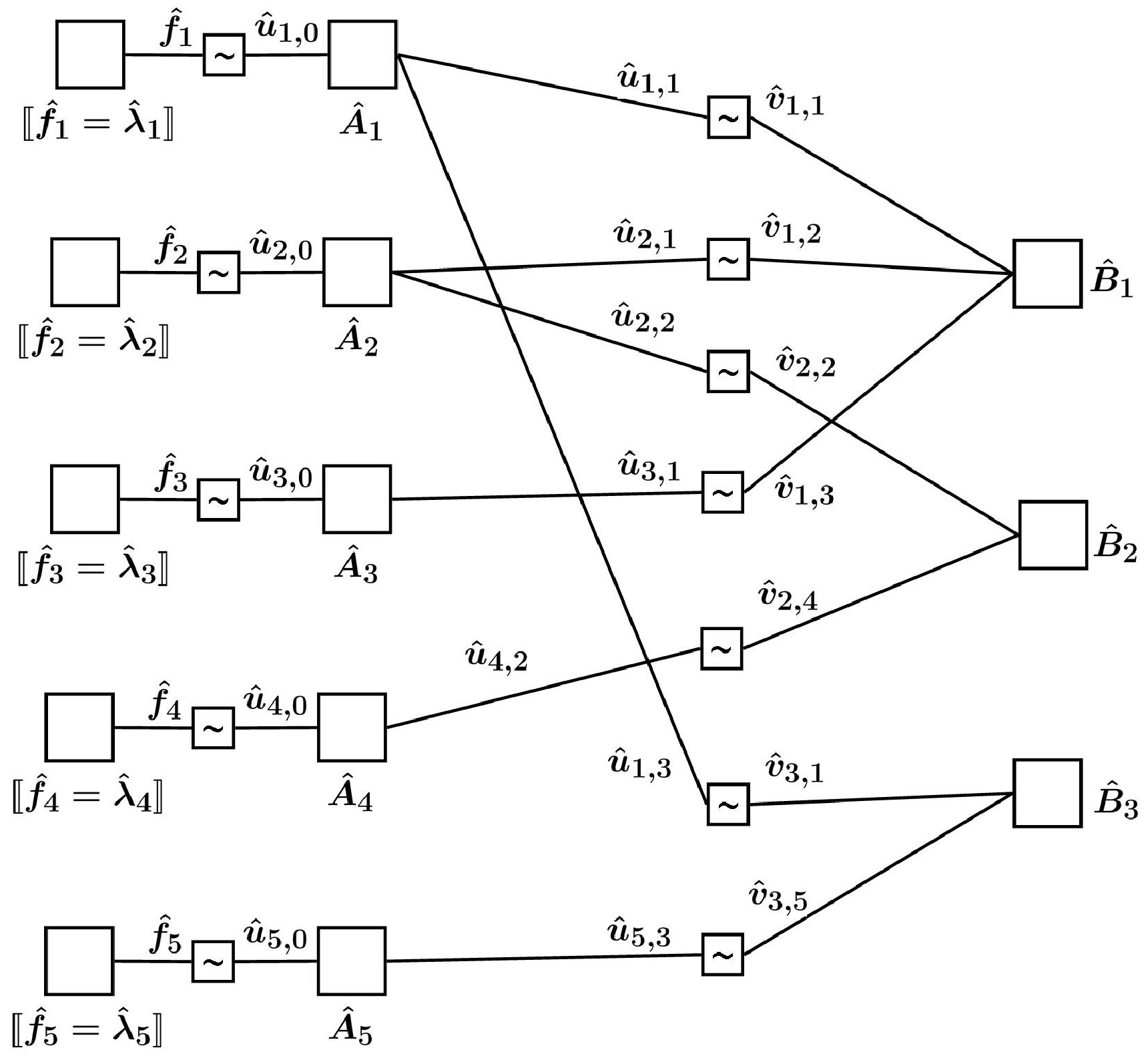
Figure 2: FFG which represents the augmented cost function of equation (11) for the example $(5,2)$ binary code.

Before deriving the dual linear program, we reformulate the PNBLPD so that this LP can be represented by an FFG. For this purpose, constraints of the PNBLPD are expressed as additive cost terms (also known as penalty terms). The rule for assigning cost to a configuration of variables is: if a given configuration satisfies the LP constraints then cost $0$ is assigned to this configuration, otherwise $+\infty$ is assigned. The PNBLPD is then equivalent to the unconstrained minimization of the following augmented cost function,

$$\sum_{i\in\mathcal{I}}{\boldsymbol{\lambda}}_{i}{\boldsymbol{f}}_{i}^{T} +\sum_{i\in\mathcal{I}}\llbracket{\boldsymbol{f}}_{i}={\boldsymbol{u}}_{i,0}\rrbracket+\sum_{(i,j)\in\mathcal{E}}\llbracket{\boldsymbol{u}}_{i,j}={\boldsymbol{v}}_{j,i}\rrbracket$$

$$+\sum_{i\in\mathcal{I}}A_{i}({\boldsymbol{u}}_{i})+\sum_{j\in\mathcal{J}}B_{j}({\boldsymbol{v}}_{j})$$ (6)

where $\forall i\in\mathcal{I}$ and $\forall j\in\mathcal{J}$ we use

$$A_{i}({\boldsymbol{u}}_{i}) \triangleq\left\llbracket\sum_{{\boldsymbol{a}}\in\mathcal{A}_{i}}\gamma_{i,{\boldsymbol{a}}}\;\Xi({\boldsymbol{a}})={\boldsymbol{u}}_{i}\right\rrbracket+\sum_{{\boldsymbol{a}}\in\mathcal{A}_{i}}\llbracket\gamma_{i,{\boldsymbol{a}}}\geq 0\rrbracket$$

$$+\left\llbracket\sum_{{\boldsymbol{a}}\in\mathcal{A}_{i}}\gamma_{i,{\boldsymbol{a}}}=1\right\rrbracket,$$

$$B_{j}({\boldsymbol{v}}_{j}) \triangleq\left\llbracket\sum_{{\boldsymbol{b}}\in\mathcal{C}_{j}}\beta_{j,{\boldsymbol{b}}}\;\Xi({\boldsymbol{b}})={\boldsymbol{v}}_{j}\right\rrbracket+\sum_{{\boldsymbol{b}}\in\mathcal{C}_{j}}\llbracket\beta_{j,{\boldsymbol{b}}}\geq 0\rrbracket$$

$$+\left\llbracket\sum_{{\boldsymbol{b}}\in\mathcal{C}_{j}}\beta_{j,{\boldsymbol{b}}}=1\right\rrbracket.$$

For ease of illustration we consider a $(5,2)$ binary code with parity-check matrix

$$\mathcal{H}=\left[\begin{array}[]{l l l l l}1&1&1&0&0\\ 0&1&0&1&0\\ 1&0&0&0&1\\ \end{array}\right]\;.$$

The augmented cost function for this code is represented by the FFG of Figure 2.

IV Dual Linear Program

The dual linear program of PNBLPD can be derived from the augmented cost function of equation (6). First we derive the dual of $A_{i}({\boldsymbol{u}}_{i})\text{ and }B_{j}({\boldsymbol{v}}_{j})$. For simplicity of exposition, we assume $\mathcal{A}_{i}=\{{\boldsymbol{p}},{\boldsymbol{q}}\}=\{(p_{0},p_{1},p_{2}),(q_{0},q_{1},q_{2})\}$. The (primal) FFG of $A_{i}({\boldsymbol{u}}_{i})$ is shown in Figure 4 and its dual is shown in Figure 4. The dual FFG is derived with the help of techniques introduced in [5] and [6].

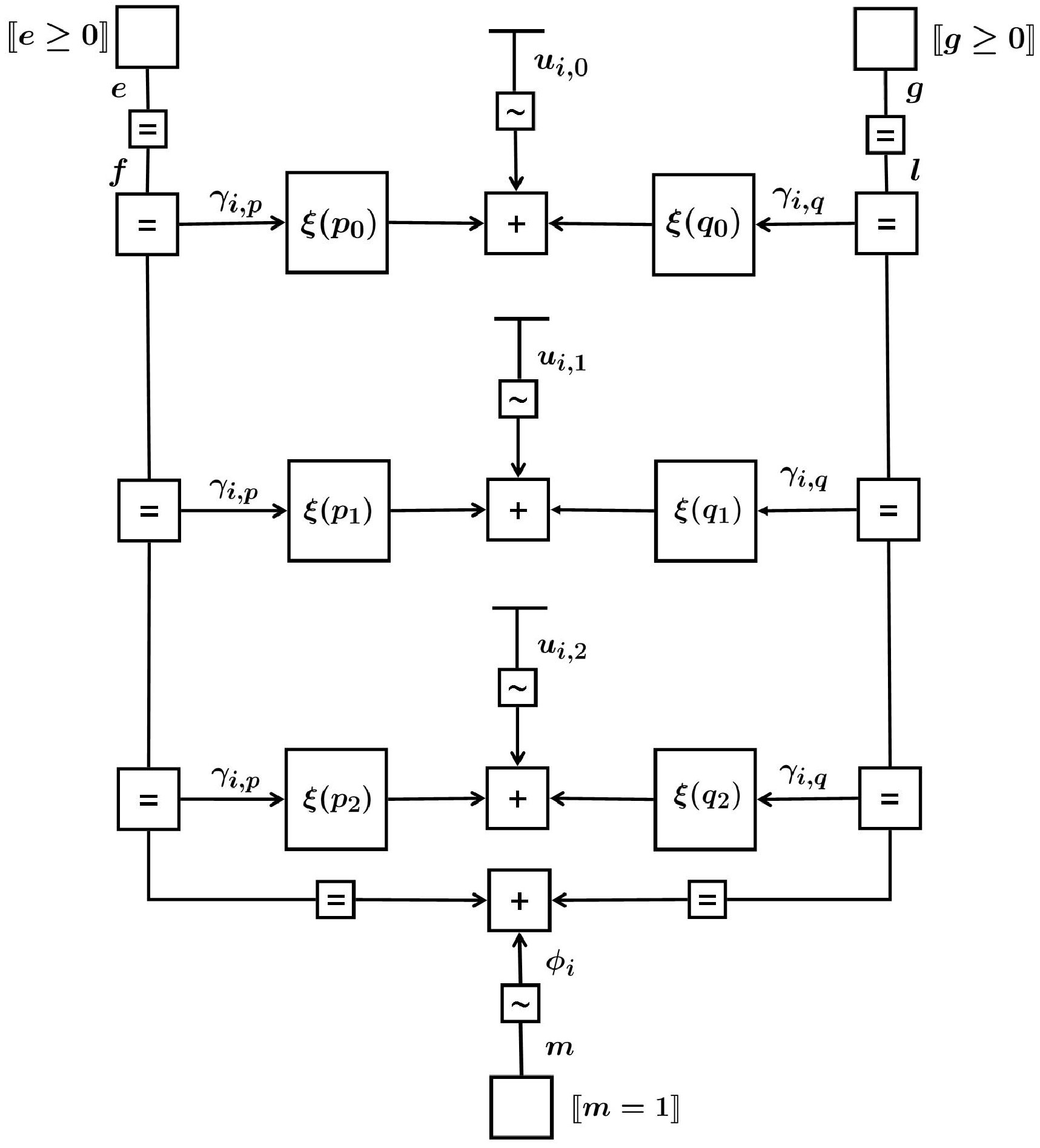
Figure 3: FFG for the function $A_{i}({\boldsymbol{u}}_{i})$. This forms a subgraph of the overall FFG of Figure 2.

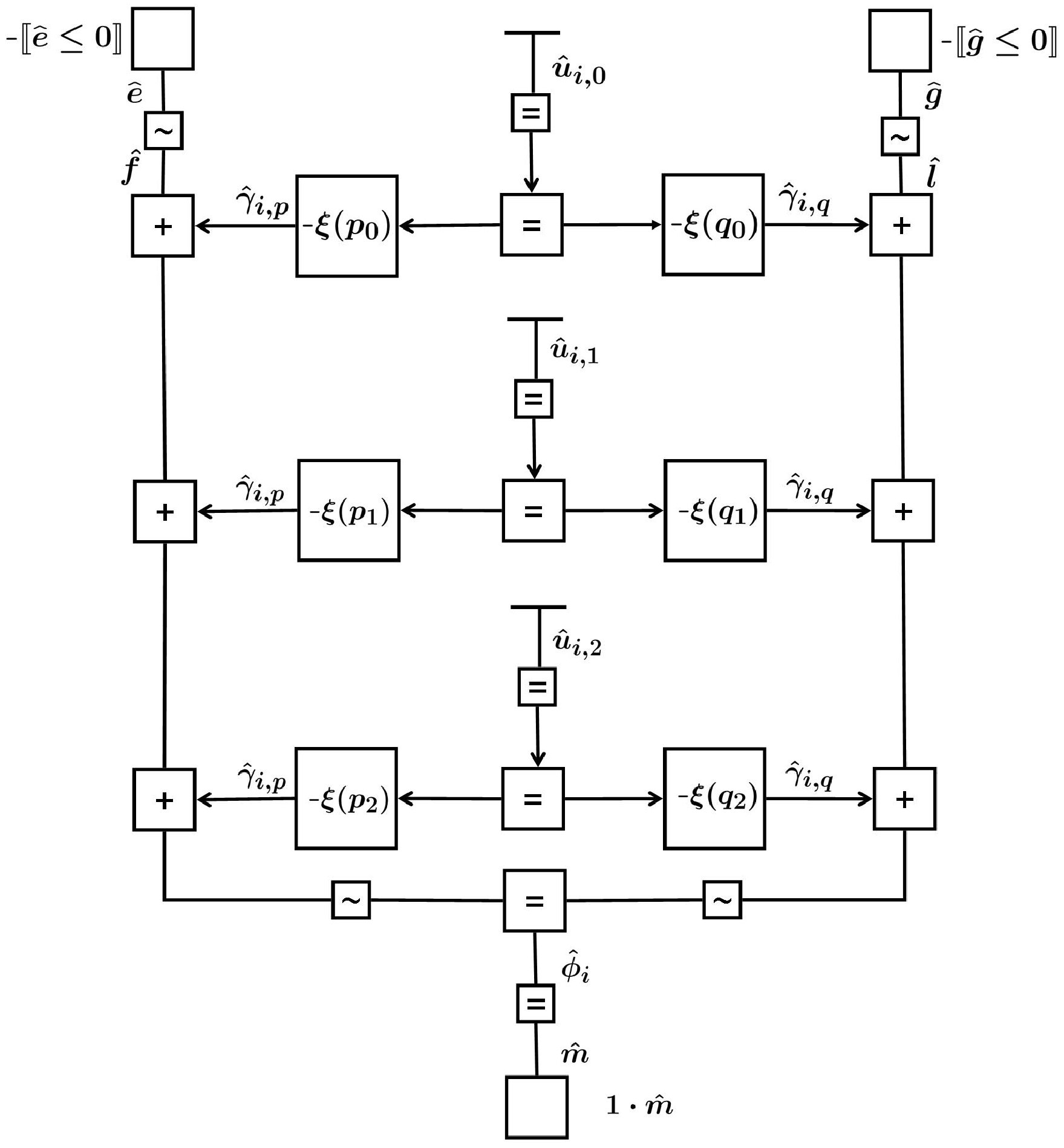
Figure 4: FFG for the function $\hat{A}_{i}(\hat{{\boldsymbol{u}}}_{i})$. This FFG is dual to that of Figure 4. Here, for any variable $x$, $\hat{x}$ denotes the dual variable.

The dual function $\hat{A}_{i}(\hat{{\boldsymbol{u}}}_{i})$ is derived from the FFG of Figure 4 as follows,

$$\hat{A}_{i}(\hat{{\boldsymbol{u}}}_{i})=\hat{m}-\llbracket\hat{e}\leq 0\rrbracket-\llbracket\hat{g}\leq 0\rrbracket$$ (8)

where $\hat{m}=\hat{\phi}_{i}$ and

$$\hat{e}=-\hat{f}=-\hat{\phi}_{i}+\langle\;-\hat{{\boldsymbol{u}}}_{i},\;\Xi({\boldsymbol{p}})\;\rangle$$

$$\Rightarrow -\left\llbracket\hat{e}\geq 0\right\rrbracket=-\left\llbracket\hat{\phi}_{i}\leq\langle\;-\hat{{\boldsymbol{u}}}_{i},\;\Xi({\boldsymbol{p}})\;\rangle\right\rrbracket$$ (9)

Similarly

$$-\llbracket\hat{g}\geq 0\rrbracket=-\left\llbracket\hat{\phi}_{i}\leq\langle\;-\hat{{\boldsymbol{u}}}_{i},\;\Xi({\boldsymbol{q}})\;\rangle\right\rrbracket$$ (10)

From equation (8), (9), (10)

$$\hat{A}_{i}(\hat{{\boldsymbol{u}}}_{i})=\hat{\phi}_{i}-\llbracket\hat{\phi}_{i}\leq\langle\;-\hat{{\boldsymbol{u}}}_{i},\;\Xi({\boldsymbol{p}})\;\rangle\rrbracket-\llbracket\hat{\phi}_{i}\leq\langle\;-\hat{{\boldsymbol{u}}}_{i},\;\Xi({\boldsymbol{q}})\;\rangle\rrbracket$$

$$\Rightarrow\hat{A}_{i}(\hat{{\boldsymbol{u}}}_{i})=\hat{\phi}_{i}-\left\llbracket\hat{\phi}_{i}\leq\min_{{\boldsymbol{a}}\in\mathcal{A}_{i}}\langle\;-\hat{{\boldsymbol{u}}}_{i},\;\Xi({\boldsymbol{a}})\;\rangle\right\rrbracket$$

The same procedure can be used to derive the dual of $B_{j}({\boldsymbol{v}}_{j})$ as

$$\hat{B}_{j}(\hat{{\boldsymbol{v}}}_{j})=\hat{\theta}_{j}-\left\llbracket\hat{\theta}_{j}\leq\min_{{\boldsymbol{b}}\in\mathcal{C}_{j}}\langle\;-\hat{{\boldsymbol{v}}}_{j},\;\Xi({\boldsymbol{b}})\;\rangle\right\rrbracket\;.$$

We use $\hat{A}_{i}(\hat{{\boldsymbol{u}}}_{i})$ and $\hat{B}_{j}(\hat{{\boldsymbol{v}}}_{j})$ to derive the dual of the LP represented by equation (6), which is in the form of the maximization of the following augmented cost function,

$$\sum_{i\in\mathcal{I}} \hat{A}_{i}(\hat{{\boldsymbol{u}}}_{i})+\sum_{j\in\mathcal{J}}\hat{B}_{j}(\hat{{\boldsymbol{v}}}_{j})-\sum_{i\in\mathcal{I}}\llbracket\hat{{\boldsymbol{f}}}_{i}=-\hat{{\boldsymbol{u}}}_{i,0}\rrbracket$$

$$-\sum_{(i,j)\in\mathcal{E}}\llbracket\hat{{\boldsymbol{u}}}_{i,j}=-\hat{{\boldsymbol{v}}}_{j,i}\rrbracket-\sum_{i\in\mathcal{I}}\left\llbracket\hat{{\boldsymbol{f}}}_{i}=-{\boldsymbol{\lambda}}_{i}\right\rrbracket$$ (11)

The augmented cost function of equation (11) for the $(5,2)$ binary code is represented by the FFG of Figure 2.

The dual of PNBLPD can now be obtained from equation (11),

DNBLPD:

max. $$\quad\sum_{i\in\mathcal{I}}\hat{\phi}_{i}+\sum_{j\in\mathcal{J}}\hat{\theta}_{j}$$

Subj. to

$$\hat{\phi}_{i} \leq\min_{{\boldsymbol{a}}\in\mathcal{A}_{i}}\left\langle-\hat{{\boldsymbol{u}}}_{i},\Xi({\boldsymbol{a}})\right\rangle ( i\in\mathcal{I}),$$

$$\hat{\theta}_{j} \leq\min_{{\boldsymbol{b}}\in\mathcal{C}_{j}}\left\langle-{\boldsymbol{\hat{v}}}_{j},\Xi({\boldsymbol{b}})\right\rangle ( j\in\mathcal{J}),$$

$$\hat{{\boldsymbol{u}}}_{i,j} =-\hat{{\boldsymbol{v}}}_{j,i} ( (i,j)\in\mathcal{E}),$$

$$\hat{{\boldsymbol{u}}}_{i,0} =-\hat{{\boldsymbol{f}}}_{i} ( i\in\mathcal{I}),$$

$$\hat{{\boldsymbol{f}}}_{i} ={\boldsymbol{\lambda}}_{i} ( i\in\mathcal{I}).$$

IV-A Softened Dual Linear Program

We make use of the soft-minimum operator introduced in [9] and derive the “Softened Dual Linear Program”. For any $\kappa\in\mathbb{R}$, $\kappa>0$, the soft-minimum operator is defined as

$$\min_{l}{}^{(\kappa)}\{z_{l}\}\triangleq-\frac{1}{\kappa}\log\left(\sum_{l}e^{-\kappa z_{l}}\right)=-{{\psi}}^{-1}\left(\sum_{l}{{\psi}}\Big{(}{-z_{l}}\Big{)}\right)$$

where $\min_{l}{}^{(\kappa)}\{z_{l}\}\leq\min_{l}\{z_{l}\}$ with equality attained in the limit as $\kappa\to\infty$. With this we define the softened dual linear program SDNBLPD which is the same as the DNBLPD except that $\min$ is replaced by $\min{}^{(\kappa)}$.

V Local Function

In SDNBLPD, $\hat{\phi}_{i}$ and $\hat{\theta}_{j}$ are involved in only one inequality and hence we can replace these inequalities with equality without changing the optimal solution (the same is true of DNBLPD). With this, let us select an edge $(i,j)\in\mathcal{E}$ and assume that the variables associated to the rest of the edges are kept constant; then the “local function” related to edge $(i,j)$ is

$${h}\left(\hat{{\boldsymbol{u}}}_{i,j}\right)=\min_{{\boldsymbol{a}}\in\mathcal{A}_{i}}{}^{(\kappa)}\left\langle-\hat{{\boldsymbol{u}}}_{i},\Xi({\boldsymbol{a}})\right\rangle+\min_{{\boldsymbol{b}}\in\mathcal{C}_{j}}{}^{(\kappa)}\left\langle-{\boldsymbol{\hat{v}}}_{j},\Xi({\boldsymbol{b}})\right\rangle\;$$ (12)

Though the soft-minimum operator is an approximation of the minimum, its advantage can be observed from equation (12). Here, the local function would be non-differentiable without use of the soft-minimum operator and as we will see in the next section, the convexity and differentiability of ${h}\left(\hat{{\boldsymbol{u}}}_{i,j}\right)$ make it easier to treat mathematically.

VI Low Complexity LP Decoding Algorithm for Nonbinary Linear Codes

If the current values of variables $\hat{{\boldsymbol{u}}}_{i,j},\hat{\phi}_{i},\hat{\theta}_{j}$ related to edge $(i,j)\in\mathcal{E}$ are replaced with the new values (at the same time keeping variables related to other edges constant) such that ${h}\left(\hat{{\boldsymbol{u}}}_{i,j}\right)$ is maximized, then we can guarantee that the dual function also increases or else remains constant at its current value. The new value $\bar{u}^{(\alpha)}_{i,j}$ for each $\hat{u}^{(\alpha)}_{i,j},\alpha\in\Re^{-}$ which maximizes ${h}\left(\hat{{\boldsymbol{u}}}_{i,j}\right)$ is given by

$$\bar{u}^{(\alpha)}_{i,j}\triangleq\operatornamewithlimits{argmax}_{\hat{u}^{(\alpha)}_{i,j}}\;{h}\left(\hat{{\boldsymbol{u}}}_{i,j}\right)\quad\left(\forall\alpha\in\Re^{-}\right)$$ (13)

Once we have calculated $\bar{{\boldsymbol{u}}}_{i,j}$, we can update the variables $\hat{\phi}_{i}$ and $\hat{\theta}_{j}$ accordingly. The calculation of $\bar{{\boldsymbol{u}}}_{i,j}$ is given in the following lemma.

Lemma VI.1

The value of $\bar{u}_{i,j}^{(\alpha)}$ of equation (13) can be calculated by

$$\quad\bar{u}_{i,j}^{(\alpha)}=\frac{1}{2}\left((V_{i,\bar{\alpha}}-V_{i,\alpha})-(C_{j,\bar{\alpha}}-C_{j,\alpha})\right)$$

where,

$$V_{i,\bar{\alpha}}\triangleq-\min_{\underset{a_{j}\neq\alpha}{{\boldsymbol{a}}\in\mathcal{A}_{i}}}{}^{(\kappa)}\left\langle-\hat{{\boldsymbol{u}}}_{i},\Xi({{\boldsymbol{a}}})\right\rangle,$$

$$V_{i,\alpha}\triangleq-\min_{\underset{a_{j}=\alpha}{{\boldsymbol{a}}\in\mathcal{A}_{i}}}{}^{(\kappa)}\left\langle-\tilde{{\boldsymbol{u}}}_{i},\Xi(\tilde{{\boldsymbol{a}}})\right\rangle,$$

$$C_{j,\bar{\alpha}}\triangleq-\min_{\underset{b_{i}\neq\alpha}{{\boldsymbol{b}}\in\mathcal{C}_{j}}}{}^{(\kappa)}\left\langle-\hat{{\boldsymbol{v}}}_{j},\Xi({\boldsymbol{b}})\right\rangle,$$

$$C_{j,\alpha}\triangleq-\min_{\underset{b_{i}=\alpha}{{\boldsymbol{b}}\in\mathcal{C}_{j}}}{}^{(\kappa)}\langle-\tilde{{\boldsymbol{v}}}_{j},\Xi(\tilde{{\boldsymbol{b}}})\rangle.$$

Here the vectors $\tilde{{\boldsymbol{u}}}_{i}$ and $\tilde{{\boldsymbol{a}}}$ are the vectors $\hat{{\boldsymbol{u}}}_{i}$ and ${{\boldsymbol{a}}}$ respectively where the $j$-th position is excluded. Similarly, vectors $\tilde{{\boldsymbol{v}}}_{j}$ and $\tilde{{\boldsymbol{b}}}$ are obtained by excluding the $i$-th position from $\hat{{\boldsymbol{v}}}_{j}$ and ${{\boldsymbol{b}}}$ respectively.

Proof:

$${h}\left(\hat{{\boldsymbol{u}}}_{i,j}\right) =\min_{{\boldsymbol{a}}\in\mathcal{A}_{i}}{}^{(\kappa)}\left\langle-\hat{{\boldsymbol{u}}}_{i},\Xi({\boldsymbol{a}})\right\rangle+\min_{{\boldsymbol{b}}\in\mathcal{C}_{j}}{}^{(\kappa)}\left\langle-{\boldsymbol{\hat{v}}}_{j},\Xi({\boldsymbol{b}})\right\rangle$$

$$=- {{\psi}}^{-1}\left(\sum_{{\boldsymbol{a}}\in\mathcal{A}_{i}}{{\psi}}\Big{(}{\left\langle\hat{{\boldsymbol{u}}}_{i},\;\Xi({\boldsymbol{a}})\right\rangle}\Big{)}\right)$$

$$-{{\psi}}^{-1}\left(\sum_{{\boldsymbol{b}}\in\mathcal{C}_{j}}{{\psi}}\Big{(}{\left\langle\hat{{\boldsymbol{v}}}_{j},\;\Xi({\boldsymbol{b}})\right\rangle}\Big{)}\right)$$

$$=- {{\psi}}^{-1}\left(\sum_{\underset{a_{j}\neq\alpha}{{\boldsymbol{a}}\in\mathcal{A}_{i}}}{{\psi}}\Big{(}{\left\langle\hat{{\boldsymbol{u}}}_{i},\;\Xi(\hat{{\boldsymbol{a}}})\right\rangle}\Big{)}+\sum_{\underset{a_{j}=\alpha}{{\boldsymbol{a}}\in\mathcal{A}_{i}}}{{\psi}}\Big{(}\langle\hat{{\boldsymbol{u}}}_{i},\;\Xi(\hat{{\boldsymbol{a}}})\rangle\Big{)}\right)$$

$$- {{\psi}}^{-1}\left(\sum_{\underset{b_{i}\neq\alpha}{{\boldsymbol{b}}\in\mathcal{C}_{j}}}{{\psi}}\Big{(}\langle\hat{{\boldsymbol{v}}}_{j},\;\Xi(\hat{{\boldsymbol{b}}})\rangle\Big{)}+\sum_{\underset{b_{i}=\alpha}{{\boldsymbol{b}}\in\mathcal{C}_{j}}}{{\psi}}\Big{(}\langle\hat{{\boldsymbol{v}}}_{j},\;\Xi(\hat{{\boldsymbol{b}}})\rangle\Big{)}\right)$$

$$=- {{\psi}}^{-1}\left(\sum_{\underset{a_{j}\neq\alpha}{{\boldsymbol{a}}\in\mathcal{A}_{i}}}{{\psi}}\Big{(}{\left\langle\hat{{\boldsymbol{u}}}_{i},\;\Xi(\hat{{\boldsymbol{a}}})\right\rangle}\Big{)}\right.$$

$$\quad\quad+\left.\sum_{\underset{a_{j}=\alpha}{{\boldsymbol{a}}\in\mathcal{A}_{i}}}{{\psi}}\Big{(}{\hat{u}_{i,j}^{(\alpha)}+\langle\tilde{{\boldsymbol{u}}}_{i},\;\Xi(\tilde{{\boldsymbol{a}}})\rangle}\Big{)}\right)$$

$$- {{\psi}}^{-1}\left(\sum_{\underset{b_{i}\neq\alpha}{{\boldsymbol{b}}\in\mathcal{C}_{j}}}{{\psi}}\Big{(}{\langle\hat{{\boldsymbol{v}}}_{j},\;\Xi(\hat{{\boldsymbol{b}}})\rangle}\Big{)}\right.$$

$$\left.\quad\quad+\sum_{\underset{b_{i}=\alpha}{{\boldsymbol{b}}\in\mathcal{C}_{j}}}{{\psi}}\Big{(}{-\hat{u}_{i,j}^{(\alpha)}+\langle\tilde{{\boldsymbol{v}}}_{j},\;\Xi(\tilde{{\boldsymbol{b}}})\rangle}\Big{)}\right)$$

$$=- {{\psi}}^{-1}\bigg{(}{{\psi}}\Big{(}{V_{i,\bar{\alpha}}}\Big{)}+{{\psi}}\Big{(}{\hat{u}_{i,j}^{(\alpha)}}\Big{)}{{\psi}}\Big{(}{V_{i,\alpha}}\Big{)}\bigg{)}$$

$$-{{\psi}}^{-1}\bigg{(}{{\psi}}\Big{(}{C_{j,\bar{\alpha}}}\Big{)}+{{\psi}}\Big{(}{-\hat{u}_{i,j}^{(\alpha)}}\Big{)}{{\psi}}\Big{(}{C_{j,\alpha}}\Big{)}\bigg{)}$$

Now to maximize ${h}\left(\hat{{\boldsymbol{u}}}_{i,j}\right)$, we set

$$\frac{\partial h\left(\hat{{\boldsymbol{u}}}_{i,j}\right)}{\partial\hat{u}_{i,j}^{(\alpha)}}=-\frac{1}{\kappa} \frac{+\kappa\;{{\psi}}\Big{(}{\hat{u}_{i,j}^{(\alpha)}}\Big{)}{{\psi}}\Big{(}{V_{i,\alpha}}\Big{)}}{{{\psi}}\Big{(}{V_{i,\bar{\alpha}}}\Big{)}+{{\psi}}\Big{(}{\hat{u}_{i,j}^{(\alpha)}}\Big{)}\;{{\psi}}\Big{(}{V_{i,\alpha}}\Big{)}}$$

$$-\frac{1}{\kappa}\;\; \frac{-\kappa\;{{\psi}}\Big{(}{-{u}_{i,j}^{(\alpha)}}\Big{)}{{\psi}}\Big{(}{C_{j,\alpha}}\Big{)}}{{{\psi}}\Big{(}{C_{j,\bar{\alpha}}}\Big{)}+{{\psi}}\Big{(}{-\hat{u}_{i,j}^{(\alpha)}}\Big{)}\;{{\psi}}\Big{(}{C_{j,\alpha}}\Big{)}}=0$$

$$\Rightarrow{{\psi}}\Big{(}{\hat{u}_{i,j}^{(\alpha)}}\Big{)}\;{{\psi}}\Big{(}{V_{i,\alpha}+C_{j,\bar{\alpha}}}\Big{)}={{\psi}}\Big{(}{-\hat{u}_{i,j}^{(\alpha)}}\Big{)}\;{{\psi}}\Big{(}V_{i,\bar{\alpha}}+C_{j,\alpha}\Big{)}$$

$$\Rightarrow\hat{u}_{i,j}^{(\alpha)}+(V_{i,\alpha}+C_{j,\bar{\alpha}})=-\hat{u}_{i,j}^{(\alpha)}+(V_{i,\bar{\alpha}}+C_{j,\alpha})\;.$$

This yields,

$$\quad\quad\quad\bar{u}_{i,j}^{(\alpha)}=\frac{1}{2}((V_{i,\bar{\alpha}}-V_{i,\alpha})-(C_{j,\bar{\alpha}}-C_{j,\alpha}))\;.$$

∎

Lemma VI.1 is a generalization of Lemma 3 of [9] to the case of nonbinary codes. One visible difference between the binary case and the present generalization is in the calculation of $V_{i,\bar{\alpha}}$ and $C_{j,\bar{\alpha}}$. Here in the case of nonbinary codes, the calculation of $V_{i,\bar{\alpha}}$ does not exclude the $j$-th entry from ${\boldsymbol{a}}\in\mathcal{A}_{i}$ and $\hat{{\boldsymbol{u}}}_{i,j}$; similarly the calculation of $C_{j,\bar{\alpha}}$ does not exclude the $i$-th entry from ${\boldsymbol{b}}\in\mathcal{C}_{j}$ and $\hat{{\boldsymbol{v}}}_{j,i}$. Note that this is not inconsistent since $\hat{u}^{({\alpha})}_{i,j}$ is never used to update itself. Here the calculation of $V_{i,\bar{\alpha}}$ and $C_{j,\bar{\alpha}}$ requires $\bar{\alpha}\in\Re\setminus\{0,\alpha\}$ and hence $\xi(\bar{\alpha})$ is always multiplied with the corresponding $\hat{u}^{(\bar{\alpha})}_{i,j}$. This ensures that $\hat{u}^{({\alpha})}_{i,j}$ is not used for calculating $\bar{u}^{(\alpha)}_{i,j}$.

As mentioned in [9], the update equation given in Lemma 3 of [9] can be efficiently computed with the help of the variable and check node calculations of the (binary) SP algorithm. Due to this, the complexity of computing $(C_{j,\bar{\alpha}}-C_{j,{\alpha}})$ is $O(d)$ for binary codes. On the other hand, in case of nonbinary codes the mapping $\Xi$ used in NBLPD transforms the nonbinary linear codes $\mathcal{A}_{i}$ (repetition code) and $\mathcal{C}_{j}$ (SPC code) into nonlinear binary codes $\mathcal{A}^{NL}_{i}=\{\Xi({\boldsymbol{a}}):\forall{\boldsymbol{a}}\in\mathcal{A}_{i}\}$ and $\mathcal{C}^{NL}_{j}=\{\Xi({\boldsymbol{b}}):\forall{\boldsymbol{b}}\in\mathcal{C}_{j}\}$ respectively. Here, the computation of $(V_{i,\bar{\alpha}}-V_{i,{\alpha}})$ and $(C_{j,\bar{\alpha}}-C_{j,{\alpha}})$ is related to the SP decoding of nonlinear binary codes $\mathcal{A}^{NL}_{i}$ and $\mathcal{C}^{NL}_{j}$. $\mathcal{A}_{i}$ and $\mathcal{C}_{j}$ are duals of each other, however such relationship between $\mathcal{A}^{NL}_{i}$ and $\mathcal{C}^{NL}_{j}$ is not so simple. Hence the computation of $(C_{j,\bar{\alpha}}-C_{j,{\alpha}})$ in the dual domain requires further investigation.

One option to compute $(C_{j,\bar{\alpha}}-C_{j,{\alpha}})$ is by going through all possible codewords of the SPC code $\mathcal{C}_{j}$ exhaustively. In this case the complexity of computing $(C_{j,\bar{\alpha}}-C_{j,{\alpha}})$ is $O(q^{(d-1)})$. However it is also possible to rewrite the equations for $C_{j,\bar{\alpha}}\;\text{ and }\;C_{j,\alpha}$ as follows,

$${{\psi}}\Big{(}C_{j,\bar{\alpha}}\Big{)}=\sum_{\underset{b_{i}\neq\alpha}{{\boldsymbol{b}}\in\mathcal{C}_{j}}}{{\psi}}\Big{(}\left\langle\hat{{\boldsymbol{v}}}_{j},\Xi({\boldsymbol{b}})\right\rangle\Big{)}$$

Similarly

$${{\psi}}\Big{(}C_{j,\alpha}\Big{)}=\sum_{\underset{b_{i}=\alpha}{{\boldsymbol{b}}\in\mathcal{C}_{j}}}{{\psi}}\Big{(}\langle\tilde{{\boldsymbol{v}}}_{j},\Xi(\tilde{{\boldsymbol{b}}})\rangle\Big{)}$$

It can be observed from the above equations that the calculation of the $C_{j,\bar{\alpha}}\;\text{and}\;C_{j,\alpha}$ is in the form of the marginalization of a product of functions. Hence it is possible to compute $C_{j,\bar{\alpha}}\text{ and }C_{j,\alpha}$ with the help of a trellis based variant of the SP algorithm. The complexity of computing $(C_{j,\bar{\alpha}}-C_{j,{\alpha}})$ with the help of the trellis of the SPC code $\mathcal{C}_{j}$ is linear in the maximum check-node degree $d$. However, this trellis based approach is still under investigation and is not used for the simulation result given in the Section VII.

We can now formulate the decoding algorithm with the help of the update equation given in Lemma VI.1. We select an edge $(i,j)\in\mathcal{E}$ and calculate $\bar{{\boldsymbol{u}}}_{i,j}$ from Lemma VI.1. Then $\hat{\phi}_{i},\;\hat{\theta}_{j}$ and the objective function are updated accordingly. One iteration is completed when all edges $(i,j)\in\mathcal{E}$ are updated cyclically. This is a coordinate-ascent type algorithm and its convergence may be proved in the same manner as in Lemma 4 of [9].

Lemma VI.2

We assume $d\geq 3$ for a given parity-check matrix $\mathcal{H}$ of the code $\mathcal{C}$. If we update all edges $(i,j)\in\mathcal{E}$ cyclically with the update equation given in Lemma VI.1, then the objective function of SDNBLPD converges to its maximum.

Proof:

The proof is essentially the same as that of Lemma 4 of [9]. ∎

The algorithm terminates after a fixed number of iterations or when it finds a codeword. Knowing the solution of SDNBLPD does not give an estimate of the codeword directly. However, an estimate of the $i$-th symbol $\hat{{\boldsymbol{c}}}_{i}$ can be obtained from the vector $\hat{{\boldsymbol{u}}}_{i,j}$. For this we define,

$$\hat{{x}}^{(\alpha)}_{i}=\sum_{j\in\mathcal{J}_{i}}-\hat{u}_{i,j}^{(\alpha)}$$

It is possible that the value of $\hat{{x}}^{(\alpha)}_{i}$ is zero. In this case, the corresponding symbol is erased. Otherwise the symbol estimate is obtained as follows:

$$\hat{{\boldsymbol{c}}}_{i} = \xi^{-1}(\hat{{\boldsymbol{f}}}_{i})$$ (14)

where

$$\hat{{f}}^{(\alpha)}_{i} = \left\{\begin{array}[]{l l}\text{1},&\text{ if }\hat{{x}}^{(\alpha)}_{i}<\text{0},\\ \text{0},&\text{ if }\hat{{x}}^{(\alpha)}_{i}>\text{0}\;.\\ \end{array}\right.$$

If more than one $\hat{{f}}^{(\alpha)}_{i}$ is assigned the value $1$, then the inverse function $\xi^{-1}$ cannot be invoked to give the estimate of ${\boldsymbol{c}}_{i}$. However, the constraints of NBLPD also enforce $\sum_{\alpha\in\Re^{-}}{{f}}^{(\alpha)}_{i}=1$, and hence we will never get such a configuration of $\hat{{f}}^{(\alpha)}_{i}$.

The advantage of using the soft-minimum operator is evident from Lemma VI.1. However, for practical implementation we are interested in $\kappa\to\infty$. As mentioned earlier, in limit of $\kappa\to\infty$, the soft-minimum operator is same as the minimum which requires less computation. The following lemma considers $\kappa\to\infty$.

Lemma VI.3

In the limit of $\kappa\to\infty$, the function $h(\hat{{\boldsymbol{u}}}_{i,j})$ is maximized by any value $\hat{{u}}_{i,j}^{(\alpha)}$ that lies in the closed interval between

$$(V_{i,\bar{\alpha}}-V_{i,{\alpha}}) -(C_{j,\bar{\alpha}}-C_{j,{\alpha}})$$ and

where

$$V_{i,\bar{\alpha}}\triangleq-\min_{\underset{a_{j}\neq\alpha}{{\boldsymbol{a}}\in\mathcal{A}_{i}}}\left\langle-\hat{{\boldsymbol{u}}}_{i},\Xi({{\boldsymbol{a}}})\right\rangle C_{j,\bar{\alpha}}\triangleq-\min_{\underset{b_{i}\neq\alpha}{{\boldsymbol{b}}\in\mathcal{C}_{j}}}\left\langle-\hat{{\boldsymbol{v}}}_{j},\Xi({\boldsymbol{b}})\right\rangle,$$

$$V_{i,\alpha}\triangleq-\min_{\underset{a_{j}=\alpha}{{\boldsymbol{a}}\in\mathcal{A}_{i}}}\left\langle-\tilde{{\boldsymbol{u}}}_{i},\Xi(\tilde{{\boldsymbol{a}}})\right\rangle C_{j,\alpha}\triangleq-\min_{\underset{b_{i}=\alpha}{{\boldsymbol{b}}\in\mathcal{C}_{j}}}\langle-\tilde{{\boldsymbol{v}}}_{j},\Xi(\tilde{{\boldsymbol{b}}})\rangle.$$

Proof:

The proof of the lemma is same as that of Lemma 5 of [9]. ∎

Now we can update edges $(i,j)\in\mathcal{E}$ cyclically where the $\bar{{\boldsymbol{u}}}_{i,j}$ is calculated according to Lemma VI.3. However, in this case, we cannot guarantee convergence of the algorithm. This is because for $\kappa\to\infty$ the objective function is not everywhere differentiable and it is not possible to use the same argument as in Lemma VI.2. This problem is also discussed in Conjecture 6 of [9]. After the algorithm terminates, equation (14) can be used to get the estimate for each symbol.

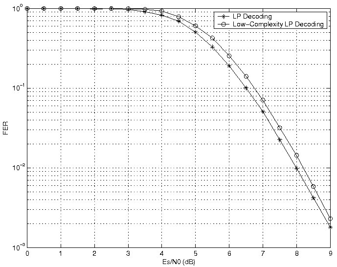
Figure 5: Frame Error Rate for the example $[80,48]$ quaternary LDPC Code under QPSK modulation. The performance of the low-complexity LP decoding algorithm is compared with that of solving NBLPD using the simplex algorithm.

VII Results

In this section we present simulation results for the proposed algorithm. The update equation of Lemma VI.3 is used for simulations. Calculation of the $(C_{j,\bar{\alpha}}-C_{j,{\alpha}})$ is carried out with exhaustive search over all codewords of SPC code $\mathcal{C}_{j}$. We use the LDPC code of length $n=80$ over $\mathbb{Z}_{4}$. This code has rate $R(\mathcal{C})=0.6$ and constant check-node degree of $5$. Its parity check matrix can be constructed as follows:

$$\mathcal{H}_{j,i}=\left\{\begin{array}[]{l l}\text{1},&\text{ if }i-j=\{\text{0, 41, 48}\}\\ \text{3},&\text{ if }i-j=\{\text{8, 25}\}\\ \text{0},&\text{ otherwise.}\end{array}\right.$$

We assume transmission over the AWGN channel where the nonbinary symbols are directly mapped to quaternary phase-shift keying (QPSK) signals. The same LDPC code was also used in [11].

Figure 5 shows the error correcting performance curve for above mentioned LDPC code. The curve marked “LP Decoding” uses the LP decoding algorithm of [11] with the simplex LP solver. All results are obtained by simulating up to $500$ frame errors per simulation point. The error correcting performance of low-complexity LP decoding algorithm is within $0.2$ dB of the LP decoder. It is important to note that the worst case time complexity of the simplex method has been shown to be exponential in the number of variables (i.e. block length). In contrast, the complexity of the low-complexity LP decoding is linear in the block length.

VIII Conclusion and Future Work

In this paper we introduced low-complexity LP decoding algorithm for nonbinary linear codes. Building on the work of Flanagan et al. [11] and Vontobel et al. [9], we derived the update equations of Lemma VI.1 & Lemma VI.3. The complexity of the proposed algorithm is linear in the block length and hence it can also be used for moderate and long block length codes. However, its complexity is dominated by the maximum check node degree and the number of elements in the nonbinary alphabet. The main problem is that of the check node calculations. The binary repetition code is the dual of the binary SPC code and this fact is utilized in binary low-complexity LP decoding algorithm to reduce the computational complexity. However, for the nonbinary case, the relationship between the corresponding nonlinear binary codes is not so simple. We are currently investigating dual domain methods for check node processing as well as variants of the sum-product algorithm which operate directly on the trellis of the nonbinary code, with the goal of leading towards a complexity reduction in the check node calculations.

IX ACKNOWLEDGMENTS

The authors would like to thank P. O. Vontobel for many helpful suggestions and comments. This work was supported in part by Claude Shannon Institute for Discrete Mathematics, Coding and Cryptography, UCD, Ireland.

References

• [1] R. G. Gallager, “Low Density Parity Check Codes,” Monograph, M.I.T. Press, 1963.
• [2] D. J. C. MacKay and R. M. Neal, “Near Shannon Limit Performance of Low Density Parity Check Codes,” Electronics Letters, vol. 33, no. 6 pp. 457-458, July 1996.
• [3] M. C. Davey and D. J. C. MacKay, “Low density parity check codes over GF(q),” IEEE Communication Letters, vol. 2, no. 6, pp. 165-167, June 1998.
• [4] G. D. Forney, Jr., “Codes on graphs: Normal realizations,” IEEE Transactions on Information Theory, vol. 47, no. 2, pp. 520-548, 2001.
• [5] P. O. Vontobel, “Kalman Filters, Factor Graphs, and Electrical Networks,” Post-Diploma Project at ETH Zurich, 2002.
• [6] P. O. Vontobel and H.-A. Loeliger, “On Factor Graphs and Electrical Networks,” Mathematical Systems Theory in Biology, Communication, Computation, and Finance, J. Rosenthal and D.S. Gilliam, eds., IMA Volumes in Math. & Appl., Springer Verlag, pp. 469-492, 2003.
• [7] H.-A. Loeliger, “An Introduction to Factor Graphs,” IEEE Signal Processing Magazine, vol. 21, no. 1, pp. 28-41, January 2004.
• [8] J. Feldman, M. J. Wainwright and D. R. Karger, “Using linear programming to decode binary linear codes,” IEEE Transactions on Information Theory, vol. 51, no. 3, pp. 954-972, March 2005.
• [9] P. O. Vontobel and R. Koetter, “Towards low-complexity linear-programming decoding,” In Proc. of 4th International Conference on Turbo Codes and Related Topics, Munich, Germany, April 3-7, 2006.
• [10] A. Globerson and T. Jaakkola, “Fixing max-product: Convergent Message Passing Algorithms for MAP LP-relaxations,” In Advances in Neural Information Processing Systems, pp. 553-560, 2007.
• [11] M. F. Flanagan, V. Skachek, E. Byrne, and M. Greferath, “Linear-Programming Decoding of Nonbinary Linear Codes,” IEEE Transactions on Information Theory, vol. 55, no. 9, pp. 4134-4154, September 2009.
• [12] Y. Maeda and K. Haruhiko, “Error Control Coding for Multilevel Cell Flash Memories Using Nonbinary Low-Density Parity-Check Codes,” 24th IEEE International Symposium on Defect and Fault Tolerance in VLSI Systems, Chicago, IL, USA, October 7-9, 2009.
• [13] D. Burshtein, “Iterative Approximate Linear Programming Decoding of LDPC Codes with Linear Complexity,” IEEE Transactions on Information Theory, vol. 55, no. 11, pp. 4835-4859, November 2009.
• [14] I. Andriyanova and K. Kasai, “Finite-Length Scaling of Non-Binary $(c,d)$ LDPC Codes for the BEC,” 2010 IEEE International Symposium on Information Theory, Dallas, TX, USA, June 13-18, 2010.