Efficient chaining of seeds in ordered trees

Abstract

We consider here the problem of chaining seeds in ordered trees. Seeds are mappings between two trees $Q$ and $T$ and a chain is a subset of non overlapping seeds that is consistent with respect to postfix order and ancestrality. This problem is a natural extension of a similar problem for sequences, and has applications in computational biology, such as mining a database of RNA secondary structures. For the chaining problem with a set of $m$ constant size seeds, we describe an algorithm with complexity $O(m^{2}\log(m))$ in time and $O(m^{2})$ in space.

1 Introduction

Comparing sequences is a basic task in computational biology, either for mining genomics database, or for filtering large sequence datasets. The exponential increase of available sequence data motivates the need for very efficient sequence comparison algorithms. A fundamental application of sequence comparison is to search efficiently in a database a set of sequences close to a query sequence. Indeed, the pairwise comparison between the query and every sequence of the database cannot practically be applied due to the quadratic time complexity of edit distance computation. A typical approach to tackle this issue is to rely on short sequences, called seeds, present in the query. These seeds can be detected very quickly in the database using indexing techniques, then a maximal set of seeds, called a chain, that tiles both the query and a sequence of the database, must be identified while conserving the same order in both sequences. Widely used programs such as BLAST [1] and FASTA [10, 13] rely on such an approach. We refer the reader to [2, 6] for surveys of sequence comparison in computational biology. From an algorithmic point of view, an optimal chain between two sequences, given $m$ seeds, can be computed in $O(m\log(m))$ time and $O(m)$ space [9] (see [12] for a recent survey).

With the recent development of high-throughput genome annotation methods, similar problems appear to be relevant for the analysis of more complex biological structures. For instance, RNA secondary structures can be modeled by a tree or a graph whose nodes are the nucleotides and whose edges are the chemical bonds between them [14]. Large databases have been constituted for this kind of biological data, such as Rfam [5]. Comparing and mining large RNA secondary structure databases is now an important computational biology problem. The initial approach to these problems relied on extensions of the notion of edit distance to ordered trees, pioneered by Zhang and Shasha [15]. The tree edit approach has been extended in several ways since then, leading either to hard problems, when a comprehensive set of edit operations is considered [8], or to algorithms with a time complexity, at best cubic, even with a minimal set of edit operations [4, 15].

Recently, Heyne et al. [7] introduced a chaining problem on another representation of ordered trees called arc annotated sequences, that they solved using dynamic programming. Their seeds are exact common patterns and they applied their algorithm for RNA secondary structure comparison: once a maximal chain of seeds between two given RNA secondary structures is detected, the regions between successive seeds are processed independently using an edit distance algorithm, which speeds up significantly the comparison process. From what we know so far, [7] is the first paper addressing a chaining problem in trees. However, when applied for chaining seeds in sequences, their algorithm complexity is higher than the best-known chaining algorithms for sequences, which raises the question of a more efficient algorithm, of both theoretical and practical interest.

After some preliminaries (Section 2 and 3), we describe in Section 4 an algorithm for finding the score of a maximum-score chain between two ordered trees (Maximal Chaining Problem) in $O(m^{2}\log(m))$ time and $O(m^{2})$ space when there are $m$ seeds of constant size, thus improving on the result of Heyne et al. [7]. We conclude with further research avenues.

2 Background and problem statement

Let $T$ be an ordered rooted tree of size $n$. Nodes of $T$ are identified with their postfix-order index from 0 to $n-1$. Thus, $n-1$ represents the root of $T$. $T_{i}$ is the subtree of $T$ rooted at $i$. We denote by $T[i,j]$ the forest induced by the nodes that belong to the interval $[i,j]$; if $i>j$, then $T[i,j]$ is empty. The partial relationship “$i$ is an ancestor of $j$” is denoted by $i\prec j$. For a tree $T$ and a node $i$ of $T$, the first leaf visited during a postfix traversal of $T_{i}$ is denoted by $l(i)$ and called the leftmost leaf of the node $i$. The ordered forest induced by the proper descendants of $i$ is denoted by $\widehat{T_{i}}=T[l(i),i-1]$.

Definition 1

Let $T$ be an ordered rooted tree:

1. Let $G=\{g_{0},\dots,g_{k-1}\}$ be an ordered set of $k$ nodes of $T$, with $0\leq g_{j}<n$. If the subgraph of $T$ induced by $G$ is connected, then $G$ is called an internal tree rooted at $g_{k-1}$ also referred as $r_{G}$.

2. The set of leaves of the internal tree $G$ is denoted by $L(G)$.

3. A node $g_{j}$ of $G$ is said to be completely inside $G$ if $g_{j}$ is not a leaf of $T$ and all its children belong to $G$. The set of nodes of $G$ that are not completely inside $G$ is called the border of $G$ and is denoted by $B(G)$.

4. Two internal trees $G^{1}$ and $G^{2}$ overlap if they share at least one node, i.e. $G^{1}\cap G^{2}\not=\emptyset$.

We now recall the central notion of valid mapping between two trees introduced in [14] for the tree edit distance. Given two trees $Q$ and $T$, a valid mapping $P$ between $Q$ and $T$ is a set of pairs of $Q\times T$ such that, if $(q_{i},t_{i})$ and $(q_{j},t_{j})$ belong to $P$, then

1. $q_{i}=q_{j}$ if and only if $t_{i}=t_{j}$,

2. $q_{i}<q_{j}$ if and only if $t_{i}<t_{j}$,

3. $q_{i}\prec q_{j}$ if and only if $t_{i}\prec t_{j}$.

In the following we use the term mapping to refer a valid mapping. Given a mapping $P$ between $Q$ and $T$, the smallest internal tree of $Q$ (resp. $T$) that contains all nodes of $Q$ (resp. $T$) belonging to a pair of $P$ is denoted by $Q_{P}$ (resp. $T_{P}$). $Q_{P}$ and $T_{P}$ are respectively called the internal trees of $Q$ and $T$ induced by $P$.

Definition 2

Let $Q$ and $T$ be two ordered trees.

1. A seed $\mathcal{M}$ between $Q$ and $T$ is a mapping between $Q$ and $T$ such that $(r_{Q_{\mathcal{M}}},r_{T_{\mathcal{M}}})\in\mathcal{M}$ and all the nodes of the border of $Q_{\mathcal{M}}$ (resp. $T_{\mathcal{M}}$) belong to a pair of $\mathcal{M}$.

2. The border (resp. leaves) $B(\mathcal{M})$ (resp. $L(\mathcal{M})$) of the seed $\mathcal{M}$ is the set of pairs $(x,y)\in\mathcal{M}$ such that $x\in B(Q_{\mathcal{M}})$ and $y\in B(T_{\mathcal{M}})$ (resp. $x\in L(Q_{\mathcal{M}})$ and $y\in L(T_{\mathcal{M}})$).

3. The size $|\mathcal{M}|$ of the seed $\mathcal{M}$ is the number of pairs its mapping contains.

4. For a set $S$ of seeds, $\|S\|$ is the sum of the sizes of the $|S|$ seeds in $S$.

Definition 3

Let $Q$ and $T$ be two ordered trees.

1. A pair $(P^{1},P^{2})$ of seeds between $Q$ and $T$ is chainable if $Q_{P^{1}}$ does not overlap $Q_{P^{2}}$, $T_{P^{1}}$ does not overlap $T_{P^{2}}$, and $P^{1}\cup P^{2}$ is a mapping.

2. A chain is a set $C=\{P^{0},P^{1},\ldots,P^{\ell-1}\}$ of seeds between $Q$ and $T$ such that any pair $(P^{i},P^{j})$ of distinct seeds in $C$ is chainable.

3. Given a scoring function $v$ for the seeds $P^{i}$, the score of a chain $C$ is the sum of the scores of its seeds: $v(C)=\sum_{i}v(P^{i})$.

4. Given a set $S$ of possibly overlapping seeds between $Q$ and $T$, $\mathcal{C}_{S}(Q,T)$ denotes the set of all possible chains between $Q$ and $T$ included in $S$.

Figure 1: An instance of the MCP problem with 6 seeds: $P^{0}=\{(2,10),(3,11)\}$, $P^{1}=\{(6,3)\}$, $P^{2}=\{(9,5)\}$, $P^{3}=\{(10,6),(11,7)\}$, $P^{4}=\{(7,4),(11,7),(12,8)\}$, $P^{5}=\{(3,1),(13,9),(14,11)\}$. If $v(P^{i})=|P^{i}|$ for every seed, an optimal chain is composed of $\{P^{1},P^{2},P^{4},P^{5}\}$ and has score $8$.

Problem. Maximum Chaining Problem (MCP):
Input: A pair $(Q,T)$ of ordered rooted trees, a set $S=\{P^{0},\dots,P^{m-1}\}$ of $m$ possibly overlapping seeds between $Q$ and $T$, and a scoring function $v$ on the seeds $P^{i}$.
Output: The maximum score chain $C$ included in $S$.

$$MCP(Q,T,S)=\max\{v(C);C\in\mathcal{C}_{S}(Q,T)\}$$

Fig. 1 shows an instance of the MCP problem with 6 seeds.

Remark 1

The notion of mapping extends naturally to ordered forests. Hence, if $S$ is a set of seeds between two forests $F_{1}$ and $F_{2}$ such that each seed is a seed between a tree of $F_{1}$ and a tree of $F_{2}$, then the MCP can naturally be extended to ordered forests.

Remark 2

To compare with chaining algorithms for sequences, we represent a sequence $u=(u_{0},\ldots,u_{n-1})$ by a unary tree, rooted at a node labeled by $u_{n-1}$, where every internal node has a single child and $u_{0}$ is the unique leaf: the sequence of nodes visited by the postfix-order traversal of this tree is exactly $u$.

Motivation and background.

As far as we know, [7] is the only work that attacks the MCP in tree structures, although the authors describe the problem in terms of arc-annotated sequences. They proposed a dynamic programming algorithm to solve the maximum chaining problem with some restrictions on the seeds (precisely, seeds are maximal exact pattern common to the considered sequences). This dynamic programming technique is different from, and in fact simpler than, the approaches used for the Maximum Chaining Problem in sequences, and, when applied to arc-annotated sequences with no arc (i.e. sequences) it can be shown this algorithm has a worst-case time complexity in $O(m^{2})$, where $m$ is the number of seeds (see Appendix).

Our main result is an algorithm that solves the Maximum Chaining Problem with a better complexity than the algorithm of [7]. After a preprocessing of the $m$ input seeds of $S$, that can be done in time $O(\|S\|)$ (we discuss in appendix the complexity of this preprocessing), our algorithm solves the Maximum Chaining Problem in $O(\|S\|\log(\|S\|)+m\|S\|\log(m))$ time and $O(m\|S\|)$ space. In particular, when applied on sequences (Remark 2), our algorithm has the same complexity than the best known algorithms for chaining seeds in sequences [12], that is $O(m\log(m))$ in time and $O(m)$ in space.

Remark 3

Without lost of generality, from now we assume that the seeds $P^{i}$ are sorted increasingly according the postfix number of their roots in $Q$, that is: $r_{Q_{P^{0}}}\leq\dots\leq r_{Q_{P^{i}}}\leq\dots\leq r_{Q_{P^{m-1}}}$. For a given chain $C$, the last seed of $C$ is then the seed with the highest postfix index in $Q$.

3 Combinatorial properties of seeds and chains

We first describe combinatorial properties of seeds and chains, that naturally lead to a recursive scheme to compute a maximum chain. Indeed, we show that given a chain $C$ and its last seed $P$, the root and border of $P$ define a partition of both $Q-Q_{P}$ and $T-T_{P}$ into pairs of forests that contain the seeds $C-\{P\}$ and form sub-chains of $C$.

Definition 4

Let $P$ be a seed on two trees $Q$ and $T$ and $(a,b;c,d)$ be a quadruple such that $l(r_{Q_{P}})\leq a<b<r_{Q_{P}}$, $l(r_{T_{P}})\leq c<d<r_{T_{P}}$ and the pair of forests $(Q[a,b],T[c,d])$ is free of $P$’s nodes ($Q_{P}\cap Q[a,b]=\emptyset$ and $T_{P}\cap T[c,d]=\emptyset$).

1. $(a,b;c,d)$ is called $P$-left-maximal if one of the following assertion is verified: (1) $a=l(r_{Q_{P}})$ and $c=l(r_{T_{p}})$, (2) there exists $(x,y)\in P$ such that $x\in Q_{a-1}$ and $y\in T_{c-1}$.

2. $(a,b;c,d)$ is called $P$-right-maximal if one of the following assertion is verified: (1) $b=r_{Q}-1$ and $d=r_{T}-1$, (2) there exists $(x,y)\in P$ such that $b+1\in Q_{x}$ and $d+1\in T_{y}$.

For example, in Fig. 1, let us consider the seed $P=P^{5}$ ; then, $(4,12;2,8)$ is $P$-left-maximal as $(3,1)\in P$, $3$ is the root of $Q_{3=4-1}$ and its image $1$ in $T$ is the root of $T_{1=2-1}$. Since $(13,9)$ is in $P$, $Q_{13}$ contains $12+1$ and $T_{9}$ contains $8+1$, assertion (2.2) of Definition 4 is also verified and $(4,12;2,8)$ is $P$-right-maximal.

Definition 5

Let $(x,y)\in B(P)$ for a seed $P$ between $Q$ and $T$. We define by $F(x,y)=\{(a_{i},b_{i};c_{i},d_{i})\}$ the set of all quadruples in $[l(x);x[^{2}\times[l(y);y[^{2}$ that are both $P$-left-maximal and $P$-right-maximal and such that there is no border node of $P$ in $Q$ (resp. $T$) on the path from $b$ to $x$ (resp. $d$ to $y$). We call this set the chainable areas of the border node $x$.

For example, let us consider a pair $(x,y)$ in $L(P)$ such that $x$ and $y$ are not a leaf of respectively $Q$ and $T$, then $F(x,y)$ represents the couple of forests $\widehat{Q_{x}}$ and $\widehat{T_{y}}$, $F(x,y)=\{(l(x),x-1;l(y),y-1)\}$. In Fig. 1, with $P=P^{4}$ and $(x,y)=(11,7)$, $F(x,y)=\{(8,10;5,6)\}$); if $(x,y)=(14,11)\in B(P^{5})-L(P^{5})$, $F(x,y)=\{(0,1;0,0),(4,12;2,8)\}$.

Definition 6

The chainable areas of a seed $P$, denoted by $CA(P)$, is the union of the sets of quadruples $F(x,y)$ for all pairs $(x,y)\in B(P)$.

Notation. For a seed $P$ (resp. chain $C$) and a chainable area $(a,b;c,d)$, we say that $P\subset(a,b;c,d)$ (resp. $C\subset(a,b;c,d)$) if, for every $(x,y)\in P$ (resp. $(x,y)$ in a seed of $C$), $x\in Q[a,b]$ and $y\in T[c,d]$.

The following property is a relatively straightforward consequence of the definitions of seeds and chainable areas.

Property 1

Given a seed $P$ between trees $Q$ and $T$, $|CA(P)|\leq 2\times|B(P)|+1$.

The next property describes the structure of any chain between two forests $Q[a,b]$ and $T[c,d]$ included in a set of $m$ seeds $S=\{P^{0},\ldots,P^{m-1}\}$. It is a direct consequence of the constraints that define a valid mapping and the fact that seeds are non-overlapping in a chain.

From now, for every $(x,y)$ of a seed $P^{j}$, we denote by $x^{j}$ the unique node $y$ of $T$ associated with $x$ in $P^{j}$. We also denote by $F_{j}(x)$ the set of quadruples $F(x,x^{j})$ for the pair of nodes $(x,x^{j})\in P^{j}$.

Property 2

Let $P^{j}$ be the last seed of a chain $C$ included into two forests $Q[a,b]$ and $T[c,d]$.

1. $C$ can be decomposed into $|CA(P^{j})|+2$ (possibly empty) distinct sub-chains: $P^{j}$ itself, $|CA(P^{j})|$ chains: for each $(e,f;g,h)\in CA(P^{j})$ a (possible empty) chain included into $Q[e,f]$ and $T[g,h]$ and a chain included into the forests $Q[a,l(r_{j})-1]$ and $T[c,l(r^{j}_{j})-1]$.

2. Moreover, $C$ is a chain of maximum score if all of its sub-chains described above are maximal.

Property 2.2 naturally leads to a recursive scheme to compute an optimal chain between two forests $Q[a,b]$ and $T[c,d]$ that ends by the last seed of a set. If $MCP^{\prime}(Q[a,b],T[c,d],\{P^{0}\dots P^{j}\})$ is the score of a maximum chain between $Q[a,b]$ and $T[c,d]$ and that contains $P^{j}$:

$$MCP^{\prime}(Q[a,b],T[c,d],\{P^{0}\dots P^{j}\})=$$ (1)

$$\left\{\begin{array}[]{lllr}0&\lx@intercol\hfil\text{if $P^{j}\not\subset(a,b;c,d)$,}\lx@intercol\\ \\ v(P^{j})&\lx@intercol+\displaystyle\sum_{(e,f;g,h)\in CA(P^{j})}MCP(Q[e,f],T[g,h],\{P^{0}\dots P^{j-1}\})\hfil\lx@intercol&\hbox{\multirowsetup\text{\hskip 20.00003ptotherwise.}}\\ &+MCP(Q[a,l(r_{j})-1],T[c,l(r^{j}_{j})-1],\{P^{0}\dots P^{j-1}\})&\\ \end{array}\right.$$

and thus $MCP(Q,T,S)$ can be computed using $MCP^{\prime}$ as follow:

$$MCP(Q[a,b],T[c,d],\{P^{0}\dots P^{j}\}) = \max_{i=0\dots j}MCP^{\prime}(Q[a,b],T[c,d],\{P^{0}\dots P^{i}\})$$ (2)

$$MCP(Q,T,S) = MCP(Q[0,r_{Q}],T[0,r_{T}],S)$$ (3)

The main challenge in designing an algorithm for the MCP is then to implement efficiently this recursive formula, that was already central in the dynamic programming algorithm of [7]. In Section 4, we will rely on the fact that for every seed $P^{j}$, $CA(P^{j})$ and, for every border node $x$ of $P^{j}$, $F_{j}(x)$, have been computed during a preprocessing phase. We discuss in Appendix the issues related to this preprocessing and we show that it can be done in $O(\|S\|)$ time and space.

4 Algorithms for the Maximal Chaining Problem

From now, we consider that we are given two ordered trees $Q$ and $T$, a set $S=\{P^{0},\ldots,P^{m-1}\}$ of seeds and a scoring score $v$ on $S$. Furthermore, we assume that the score $v(j)$ of a seed $P^{j}$ can be accessed in constant time and the seeds of $S$ are given as a list $I$ of triples $(i,f,j)$ such that: (1) $i$ is the postfix number of either the root of $P_{Q}^{j}$ or a border node of $P_{Q}^{j}$ (ie. $i\in B(P_{Q}^{j})\cup r(P_{Q}^{j})$) and (2) $f$ is a flag indicating if $i$ is either border ($f=0$) or root ($f=1$) for $P_{Q}^{j}$. Thus if $i$ is both in $B(P_{Q}^{j})$ and the root of $P_{Q}^{j}$ then $i$ appears in two distinct triples. Moreover, for a node $i$ in $Q$ belonging to a seed $P^{j}$, we assume that the corresponding node in $T$, $i^{j}$ (or more precisely its postfix number in $T$) can be accessed in constant time. Finally, for every node $i$ in $Q$ and $T$, its leftmost leaf $l(i)$ is also supposed to be accessed in constant time.

As a preprocessing, $I$ is sorted in lexicographic order. Thus, if a node is both in the border and root of $P^{j}$, it first appears in $I$ as a border, then as a root. This sorting can be done in $O(||S||\log(||S||))$ time. In our algorithms, we visit successively the elements of $I$ in increasing order, and a seed $P^{j}$ is said to be processed after its root has been processed (i.e. the current element of $I$ is greater than $(r_{j},1,j)$ for the order defined above).

In the following, we first introduce a simple but non optimal algorithm to compute the MCP between $Q$ and $T$ which does not require any special data structure. In a second step, we will present a more efficient method based on a simple modification of this algorithm.

4.1 A simple non optimal algorithm

In order to compute in constant time the partial $MCP$ for any pair of forests in $CA(P^{j})$ as described in equation (1), we introduce a data structure $M$ indexed by quadruples of integers $(a,b;c,d)$ defining the forests $Q[a,b]$ and $T[c,d]$. These quadruples $(a,b;c,d)$ belong to a set $Y=Y_{1}\cup Y_{2}\cup Y_{3}$ defined as follows:

$$Y_{1}=\bigcup_{j=0}^{m-1}CA(P^{j}),\ Y_{2}=\{(0,r_{Q},0,r_{T})\},$$

$$Y_{3}=\{(a,l(r_{j})-1;c,l(r_{j}^{j})-1)\text{ s.t. }\exists(b,d)\text{ s.t. }(a,b;c,d)\in Y_{1}\cup Y_{2}\text{ and }P^{j}\subset(a,b;c,d)\}$$

In algorithm 1, the function Update allows to replace the value of $M[a,b,c,d]$ by a real number $w$ if $w$ is greater than $M[a,b,c,d]$. We also use an array $V$ of $m$ integers to store the intermediate quantities of $MCP^{{}^{\prime}}$. The correctness of the algorithm relies on the following invariants for the two data structures $V$ and $M$, that we prove later:

• After $P^{j}$ has been processed, then $M[a,b,c,d]=MCP(Q[a,b],T[c,d],$$\{P^{0},\dots,P^{j}\})$ for every $(a,b;c,d)\in Y$.

• After $P^{j}$ has been processed, then $V[j]=MCP^{\prime}(Q,T,\{P^{0},\dots,P^{j}\})$.

Algorithm 1 $MCP_{1}$: compute the score of a maximal chain.

⬇

1for $j$ from $0$ to $m-1$ do $V[j]=v(j)$

2foreach $(a,b;c,d)\in Y$ do $M[a,b,c,d]=0$

3foreach $(i,f,j)$ in $I$ do

4 if $f=0$ then # i.e. $(i,i^{j})\in B(P^{j})$

5 foreach $(a,b;c,d)\in F_{j}(i)$ do $V[j]=V[j]+M[a,b,c,d]$

6 else # i.e. $f=1$ and $i$ is the root of $Q_{P^{j}}$, $i=r_{j}$

7 foreach $(a,b;c,d)\in Y_{1}\cup Y_{2}$ s.t. $P^{j}\subset(a,b;c,d)$ do

8 Update $M[a,b,c,d]$ with $w=V[j]+M[a,l(r_{j})-1,c,l({r^{j}_{j}})-1]$

9 foreach $P^{g}\subset(r_{j}+1,b;r^{j}_{j}+1,d)$ do

10 Update $M[a,l(r_{g})-1,c,l({r^{g}_{g}})-1]$ with $w$

11 $V[j]=V[j]+M[0,l(r_{j})-1,0,l(r^{j}_{j})-1]$

12return $\max_{j}V[j]$

Correctness of the algorithm.

Obviously, V1 implies that $\max_{j}V[j]$ contains the score of the maximal chain (equations (2) and (3)). Let us assume now that M1 is satisfied. If the seed $P^{j}$ has been processed, then $V[j]$ contains the sum of $v(j)$ (line 1), the MCP scores of the chainable areas of all its border nodes (line 5) and the MCP score between forests $Q(0,l(r_{j})-1)$ and $T(0,l(r^{j}_{j})-1)$ (line 11). From Property 2 and (1), $V[j]=MCP^{\prime}(Q,T,\{P^{0},\dots,P^{j}\})$ and V1 is satisfied.

We prove M1 by induction. Initially, since no seed has been processed, line 2 ensures that M1 is satisfied. Now let us assume that M1 is satisfied for all processed seeds $\{P^{0},\ldots,P^{j-1}\}$ and the input $(i,1,j)$ is being processed. If $P^{j}\not\subset(a,b;c,d)$, then by induction, M1 is satisfied for $M[a,b,c,d]$. Otherwise, the loop in lines 7 and 8 ensures that M1 is satisfied for all entries $M[a,b,c,d]$ such that $(a,b;c,d)\in Y_{1}\cup Y_{2}$, as $(a,l(r_{j})-1;c,l({r^{j}_{j}})-1)$ does not contain $P^{j}$ ; thus by induction M1 is satisfied for this index. Finally, the loop in line 9 update all $(a,b;c,d)\in Y_{3}$ including $P^{j}$,and M1 is satisfied for all entries of $M$.

Complexity analysis.

From Property 1, the space required to encode the entries of $M$ indexed by $Y_{1}$ is in $O(\|S\|)$. The space required to encode the entries of $M$ indexed by $Y_{3}$ is in $O(m^{2})$, as for every pair of seeds $P^{i}$ and $P^{j}$, there is at most one chainable area of $CA(P^{i})$ that contains $P^{j}$.

We now address the worst-case time complexity. We do not factor the preprocessing required to compute the $F_{j}$ and $CA$ and we assume $I$ has been sorted in time $O(\|S\|\log(\|S\|))$. The amortized cost of lines 4–5 is $O(\|S\|)$, as each chainable area is considered once, there are $O(\|S\|)$ such areas, and we assumed we can access them in amortized constant time. A naive implementation of lines 6–11 would require $O(m^{2}\|S\|)$ operations: indeed, there are $m$ iterations of the loop in line 6, the loop in line 7 considers only entries indexed by $Y_{1}\cup Y_{2}$ (there are $O(\|S\|)$ such entries) and the loop on line 9 iterates $O(m)$ times. However, we can notice that there are $O(m)$ entries $(a,b;c,d)\in Y_{1}\cup Y_{2}$ such that $P^{j}\subset(a,b;c,d)$, and it is possible to preprocess $I$ in time and space $O(m\|S\|)$ in such a way that the loop in line 7 can be implemented to perform $O(m)$ iterations, leading to a total time complexity of $O(m\|S\|+m^{3}+\|S\|\log(\|S\|))$ (respectively for the preprocessing, the main algorithm and sorting the input).

4.2 A more efficient algorithm

The key ideas are to access less entries from $M$ (while maintaining property M1 on the remaining entries though) and to complement $M$ with a data structure $R$ that can be queried in $O(\log(m))$ instead of $O(1)$, but whose maintenance does not require a loop with $O(m^{2})$ iterations. Formally, let $X=\{(a,c)\text{ s.t. }\exists(a,b;c,d)\in Y_{1}\cup Y_{2}\}$ and $R$ be a data structure indexed by $X$ such that for a given index $(a,c)\in X$, $R[a,c]$ is a set of pairs $(j,s)$ where $j$ is the index of the seed $P^{j}$ and $s$ is the score of the chain in $Q[a,r_{j}],T[c,r_{j}^{j}]$ that ends with $P^{j}$. Roughly, $M$ is used to access, still in $O(1)$ time, the values $MCP(a,l(r_{j})-1,c,l(r^{j}_{j})-1,\{P^{0}\dots P^{j-1}\})$ required to compute $MCP^{\prime}$ in equation (1) and $R[a,c]$ is used to access, in time $O(\log(m))$, the scores of the best chains included in $(Q[a,r_{Q}],T[c,r_{T}])$ (the values $MCP(Q[e,f],T[g,h],\{P^{0}\dots P^{j-1}\})$ in equation (1)) and replace the entries $M[a,b,c,d]$ with $(a,b;c,d)\in Y_{1}\cup Y_{2}$ that were used in the previous algorithm.

Finally, the algorithm iterates on a list of triples $J=I\bigcup\left(\cup_{j=0}^{m-1}(l(r_{j}),-1,j)\right)$, sorted using the lexicographic order than in the previous section, with the following modification: if we have two seeds $P^{j}$ and $P^{g}$ with $g>j$ such that $(l(r_{j}),l(r^{j}_{j}))=(l(r_{g}),l(r^{g}_{g}))$ then only $(l(r_{j}),-1,j)$ occurs in $J$. This preprocessing requires $O(||S||\log(||S||))$ time.

Algorithm 2 $MCP_{2}(Q,T,S,v)$: compute a maximal chaining from $S$.

⬇

1for $j$ from $0$ to $m-1$ do $V[j]=v(j)$

2foreach $(a,b;c,d)\in Y_{3}$ do $M[a,b,c,d]=0$

3foreach $(a,c)\in X$ do $R[a,c]=\emptyset$

4foreach $(i,f,j)$ in $J$ do

5 if $f=-1$ then # $i=l(r_{j})$

6 foreach $(a,c)\in X$ s.t. $a,c<l(r_{j}),l(r^{j}_{j})$ do

7 $M[a,l(r_{j})-1,c,l({r^{j}_{j}})-1]$= value $s$ of the last $(y,s)$ of $R[a,c]$ s.t. $r_{y}^{y}<l({r^{j}_{j}})$

8 else if $f=0$ then # $(i,i^{j})\in B(P^{j})$

9 foreach $(a,b;c,d)\in F_{j}(i)$ do

10 Add to $V[j]$ the value $s$ of the last entry $(y,s)$ of $R[a,c]$ s.t. $r_{y}^{y}\leq d$

11 else # $f=1$ and $i$ is the root of $Q_{P^{j}}$, $i=r_{j}$

12 foreach $(a,c)\in X$ s.t. $a,c<l(r_{j}),l({r^{j}_{j}})$ do

13 $w=V[j]+M[a,l(r_{j})-1,c,l({r^{j}_{j}})-1]$

14 Insert entry $(j,w)$ into $R[a,c]$ and update $R[a,c]$ as follow:

15 Find the last entry $(y,s)$ s.t. $r_{y}^{y}<r_{j}^{j}$

16 if $s<w$ then

17 Insert $(j,w)$ just after $(y,s)$ in $R[a,c]$

18 Remove from $R[a,c]$ all entries $(z,t)$ s.t. $r_{j}^{j}\leq r_{z}^{z}$ and $t<w$

19 $V[j]=V[j]+M[0,l(r_{j})-1,0,l(r^{j}_{j})-1]$

20return $\max_{j}V[j]$

Correctness of the algorithm.

We consider the following invariants.

• After $P^{j}$ has been processed, then $M[a,b,c,d]=MCP(Q[a,b],T[c,d],$$\{P^{0},\dots,P^{j}\})$ for every $(a,b;c,d)\in Y_{3}$.

• After $P^{j}$ has been processed, then $V[j]=MCP^{\prime}(Q,T,\{P^{0},\dots,P^{j}\})$.

• After $P^{j}$ has been processed, then for all $(a,c)\in X$, $R[a,c]$ contains all $(y,s)$ that satisfies

  • $y\leq j\text{ and }s=MCP^{\prime}(Q[a,r_{y}],T[c,r^{y}_{y}],\{P^{0},\ldots,P^{y}\})$.

  • $\forall(z,t)\in R[a,c],~{}r_{z}^{z}<r_{y}^{y}\Rightarrow t<s$.

• $\forall(a,c)\in X$, $R[a,c]$ is totally ordered as follows: $(y,s)<(z,t)$ iff $r_{y}^{y}<r_{z}^{z}$.

We first assume that R1 and R2 are satisfied. As previously, if V1 is satisfied, then the algorithm computes $MCP(Q,T,S)$. The initialization line 1 ensures that $V[j]$ contains $v(j)$. Next to prove V1 we only need to show that when we process a border $i$ of a seed $P^{j}$, in line 10 we add to $V[j]$ the best chains of each chainable area $(a,b;c,d)$ of the border; it follows from (1) the fact that every seed $P^{j+e}$ with $e>0$ does not belong to the forest $Q[a,b]$ (because $b<i\leq r_{j+e}$) and thus can not belong to a chain in the $(a,b;c,d)$ area, (2) the fact that the score of this chain is present in $R[a,c]$ (from R1) and (3) that fact it is the last entry $(y,s)$ such that $r_{y}^{y}\leq d$ (from R2).

M2 is similar to M1 but restricted to entries $M[a,b,c,d]$ such that $(a,b;c,d)\in Y_{3}$. To check it is satisfied, we only need to focus on line 7, as it is the only line that updates $M$. For entries $M[a,b,c,d]$ such that $a\geq l(r_{j})$ or $c\geq l(r_{j}^{j})$, then $M[a,b,c,d]=0$ due to the initialisation in line 1. For all other entries, M2 follows immediately from R1 and R2, using argument similar to the previous ones.

Finally, we need to check that R1 and R2 are satisfied. First, as previously, in the case where $a\geq l(r_{j})$ or $c\geq l(r_{j}^{j})$, $R[a,c]=\emptyset$ which is ensured by the initialisation in line 3. So we need only to consider the case where $a,c<l(r_{j}),l({r^{j}_{j}})$, that is handled in lines 11 to 18. Every seed $P^{y}$ such that $y<j$ has already been processed and $s=MCP^{\prime}(Q[a,r_{y}],T[c,r^{y}_{y}],\{P^{0},\ldots,P^{y}\})$ can not be modified after $P^{y}$ has been processed, so lines 12 and 13, together with M2, ensure that $(y,s)$ has been inserted into $R[a,c]$ previously, and the same argument applies if $y=j$. Entries $(z,t)$ removed at line 18 do not belong to any of these $(y,s)$, which implies that R1.a and R1.b, and so R1, are satisfied. R2 is obviously satisfied from the position where $(j,w)$ is inserted into $R[a,c]$ in line 17.

Complexity analysis.

The space complexity is given by the space required for structures $M$ and $R$. $M$ requires a space in $O(m^{2})$ as it is indexed by $Y_{3}$. $R$ requires a space in $O(m\|S\|)$, as $|Y_{1}\cup Y_{2}|\in O(\|S\|)$ and for each seed $P^{j}$, an entry $(j,s)$ is inserted at most once in each $R[a,c]$. All together, the space complexity is then $O(m^{2}+m\|S\|)=O(m\|S\|)$.

We now describe the time complexity. First, note that following the technique used for computing maximal chains in sequence [6, 9, 12], the structures $R[l_{Q},l_{T}]$ can be implemented using classical data structures such as AVL or concatenable queues supporting query requests, insertions, successor and, predecessor and deletions in a set of $n$ totally ordered elements in $O(\log(n))$ worst-case time.

Now, we analyse the complexity of lines 5 to 7. The loop of line 6 is performed at most $O(m\|S\|)$ times and each iteration requires $O(\log(m))$ in time (line 7), which gives an amortized time complexity of $O(m\|S\|\log(m))$.

Line 10 is applied at most once for each of the $O(\|S\|)$ chainable area $F_{j}(i)$ (Property 1), and each iteration requires $O(\log(m))$, which gives an $O(\|S\|\log(m))$ amortized time complexity.

Finally, we analyse the complexity of lines 11 to 19. First, we do not consider the operation in line 18. The number loop starting in line 12 is performed in $O(m)$, and the complexity of each loop is in $O(\|S\|)$. The cost of the operations performed during each iteration is $O(\log(\|S\|))$ (lines 13 and 16 are both performed in $O(1)$ and lines 14 and 15 in time $O(\log(\|S\|)$). The total time complexity of this part, without considering line 18, is then $O(m\|S\|\log(\|S\|))$. To complete the time complexity analysis, we show that the amortized complexity of line 18 is in $O(m\|S\|)$. Indeed, it follows from R2 that all entries removed in one step are consecutive in the total order on $R[a,c]$ defined in R2. Hence, if one call to line 18 removes $k$ elements from $R[a,c]$, it can be done in $O((k+2)\log(m))$ time, as the successor of a given element can be retrieved in $O(\log(m))$ time. As every element of $R$ is removed at most once during the whole algorithm, this leads to an amortized complexity of $O(m\|S\|\log(m))$ for line 18. Alltogether, our algorithm solves computes $MCP(Q,T)$ in time $O(m\|S\|\log(m))$, using standard data structures and after a preprocessing in time $O(\|S\|\log(\|S\|))$ to compute the chainable areas and to sort $J$.

Additional remarks.

If we consider that $Q$ and $T$ are sequences, or, as described in Section 2, unary trees, then each of the two trees has a single leaf and each seed is unambiguously defined by its root and border, which implies that$\|S\|=m$. There is only one $R[a,c]$, as $a=c=0$, that contains $O(m)$ entries. Hence, all loops that were iterating on $R$ have now a single iteration, which reduces the time complexity by a factor $m$ to $O(\|S\|\log(m))=O(m\log(m))$.

In the complexity analysis above, we followed the approach used for expressing the complexity of chaining in sequences, as we expressed the complexity only in terms of the size of the seeds. To express the complexity of our algorithm in terms of the size of $Q$ and $T$, a finer analysis of the data structure $R$ and of the number of different chainable areas leads to the following result: the worst-case space complexity of our algorithm is $O(|Q|^{2}|T|^{2})$ (similar to the algorithm of Heyne et al.), and its worst-case time complexity is in $O(\|S\|\log(\|S\|)+|Q||T|\log(|T|)(|Q||T|+m))$, to compare with the complexity of the Heyne et al algorithm that is in $O(\|S\|\log(\|S\|)+|Q|^{2}|T|^{2}(|Q||T|+m))$ (see details in the Appendix). This alternative complexity analysis is mostly of theoretical interest as in practice, for RNA analysis, one can expect that $m\ll|Q||T|$.

5 Conclusion

The current paper describes algorithms to solve chaining problems in ordered trees. With respect to similar problems in sequences, these methods exhibit a linear factor increase both in time and space. Chains so obtained can be used to speed-up RNA structure comparisons, as illustrated in [7, 11].

A natural question related to chaining problems, that, as far as we know, has not been considered in the case of sequences, is to decide whether a given seed $P$ of a set of seeds $S$ belongs to any optimal chains or not. However a trade-off between quality and speed may have to be find. Indeed, identifying these always optimal seeds would ensure a good quality of the chains, whereas the high complexity of these identifications would slow down the detection of similar structures in a large database.

Acknowledgements. Pacific Institute for Mathematical Sciences (PIMS, UMI CNRS 3069), Agence Nationale pour la Recherche project BRASERO (ANR-06-BLAN-0045), Natural Sciences and Engineering Research Council of Canada (NSERC), Multiscale Modeling of Plants associated team (INRIA).

Appendix: remarks on the dynamic programming algorithm of Heyne et al.

This appendix proposes a comparison of the worst-case time complexity between chaining algorithms proposed in the current paper and in [7].

Time complexity of Heyne et al. algorithm [7]

Heyne et al. algorithm [7] considers pairs $(S_{1},S_{2})$ of arc-annotated sequences, of respective length $n_{1}$ and $n_{2}$.

This algorithm is based on processing holes in subsequences corresponding to seeds, where a hole in an arc-annotated sequence is a part of the subsequence spanned by a seed that does not belong to the seed. In trees, holes correspond to the chainable areas of the border nodes of a seed. The complexity of this algorithm is in $O(hn_{1}n_{2})$ where $h$ is the number of different holes, $n_{1}$ and $n_{2}$ corresponds respectively to the hole size in $S_{1}$ and $S_{2}$. Due to the constraints on the definition of seeds proposed in [7] (connected nucleotides in RNA structure), authors claim a time complexity of $O(n_{1}^{2}n_{2}^{2})$ as $h$ is bounded by $O(n_{1}\times n_{2})$ [7].

Actually, this complexity do not take into account the time required to establish the holes and to sort them (holes are treated in a specific order). Thus, the total time complexity of this algorithm is $O(\|S\|\log\|S\|+h\times n_{1}\times n_{2})$ where $O(\|S\|)$ is the sum of seed sizes.

A worst-case complexity analysis

In the following, we propose an analysis of the complexity of Heyne et al. algorithm [7] in the case of more general seeds.

This algorithm uses dynamic programming tables indexed by holes (in fact pairs of holes, one in each sequence defined by a seed). Given a hole $h$ induced by a seed and defined by the sequence $S_{1}[h^{L1},h^{R1}]$ in $S_{1}$ and the sequence $S_{2}[h^{L2},h^{R2}]$ in $S_{2}$, $D^{h}(j,l)$ is the best chain included in $S_{1}[h^{L1},j]$ in $S_{1}$ and $S_{2}[h^{L2},l]$ in $S_{2}$. Each hole is then processed independently from the other ones (in an order ensuring required information have already been computed), in order to fill the table $D^{h}$, using the following dynamic programming equation:

$$D^{h}[j,l]=\max\{D^{h}(j-1,l),D^{h}(j,l-1),\max_{\begin{subarray}{c}\text{seed }P\in h\\ \text{st.}P\text{ ends on }j,l\end{subarray}}\{D^{h}(p-1,q-1)+S_{P}\}\}$$

$$S_{P}=v(P)+\sum_{h\in\text{Holes of $P$}}D^{h}(h^{R1},h^{R2})$$

where, $p$ (resp. $q$) is the first base of seed $P$ in $S_{1}$ (resp. $S_{2}$) and $S_{P}$ is the score of the best chain included in the subsequences spanned by $P$ in $S_{1}$ and $S_{2}$ and ended by $P$.

We can easily transpose this recurrence on trees, using article notation, as follow:

$$D^{h=(a,b,c,d)}[j,l]=\max\left\{\begin{array}[c]{l}D^{h}(j-1,l),\\ D^{h}(j,l-1),\\ \max_{\begin{subarray}{c}\text{seed }P\subset(a,j,c,l)\\ \text{st.}(r_{P},r^{P}_{P})=(j,l)\end{subarray}}\{D^{h}(l(r_{P})-1,l(r^{P}_{P})-1)+S_{P}\}\end{array}\right\}$$

$$S_{P}=v(P)+\sum_{(a,b,c,d)\in CA(P)}D^{(a,b,c,d)}[b,d]=MCP^{\prime}(Q_{r_{P}},T_{r^{P}_{P}},P^{0...P})$$

First, let us remark that the computation of one dynamic programming matrix can be done in $O(n_{1}n_{2}+m)$ as the matrix has at most $n_{1}\times n_{2}$ entries and the search of the seeds $P$ which ends on $j,l$ requires a pre-processing in $O(m)$.

Thus, assuming that holes have already been computed, the total time complexity is $O(\|S\|\log(\|S\|)+h\times(n_{1}n_{2}+m)+\|S\|)$ (ie. complexity of sorting of the holes plus the computation cost of $D^{h}$ plus the computation cost of $S_{P}$).

In [7], authors design seeds that are connected nucleotides in the RNA secondary structure either by backbone bond or base-pair bond. Hence, $h$ is bounded by $n_{1}n_{2}$ and the worst-case time complexity is $O(\|S\|\log(\|S\|)+n_{1}n_{2}\times(n_{1}n_{2}+m)+\|S\|)$.

If we impose seed nodes to be connected in the trees (and not in RNA), which is a special case of our seeds but different from the seeds developed by Heyne et al., the number of different holes would be $O(n_{1}^{2}n_{2}^{2})$ in the worst case (all possible quadruplets $(a,b,c,d)$). The overall complexity of the dynamic programming algorithm then becomes in the worst case:

$$O(\|S\|\log(\|S\|)+n_{1}^{2}n_{2}^{2}(n_{1}n_{2}+m)+\|S\|).$$

Time complexity of Algorithm 2

To establish the worst-case complexity of Algorithm 2, we have to study the cost of the algorithm for each $f$ values. To ease the reading, we denote by $n_{1}$ the size of $Q$ and $n_{2}$ the size of $T$. Without loss of generality, we furthemore assume that $n_{2}\leq n_{1}$.

Following invariants $R1$ and $R2$, each list of $R$ contains at most $min(m,n_{2})$ elements, as there are no $(y,s),(y^{\prime},s^{\prime})\in R[a,c]$ s.t. $r^{y}_{y}=r^{y^{\prime}}_{y^{\prime}}$, and $|X|\leq min(\|S\|,n_{1}n_{2})$. Thus, in the worst-case, we have at most $O(n_{1}^{2}n_{2}^{2})$ different chainable areas, $|R|=O(n_{1}n_{2})$, for all $(a,c)$: $|R[a,c]|=O(n_{2})$ and $|X|=O(n_{1}n_{2})$.

• line 5: Over the whole execution of the algorithm each $M[a,l(r_{j})-1,c,l(r^{j}_{j})-1]$ is computed only once for all possible quadruplets as there is no $(i,f,j)$, $(i^{\prime},f^{\prime},j^{\prime})\in J$ such that $(l(r_{j}),l(r^{j}_{j}))=(l(r_{j^{\prime}}),l(r^{j^{\prime}}_{j^{\prime}}))$. Each computation require a search in $R[a,c]$ that can be done in $O(log(n_{2}))$. Thus, the total time complexity for this case is $O(n_{1}^{2}n_{2}^{2}log(n_{2}))$.

• line 8: The computation line 10 can be store in a dedicated array $M^{\prime}$ such that the best chain of the area $(a,b,c,d)$ is computed only once. Thus, over all the execution of the algorithm, each different chainable area requires a search into a $R[a,c]$ and the total time complexity for this case is $O(\|S\|+n_{1}^{2}n_{2}^{2}\log(n_{2}))$.

• line 11: This case is run once peer seeds, so $O(m)$ times. Each run cost $O(n_{1}n_{2}\log(n_{2}))$ and the total time complexity is $O(mn_{1}n_{2}\log(n_{2}))$.

From above, we conclude that the worst-case time complexity of our algorithm is

$$O(\|S\|\log(\|S\|)+n_{1}^{2}n_{2}^{2}log(n_{2})+\|S\|+n_{1}^{2}n_{2}^{2}\log(n_{2})+mn_{1}n_{2}\log(n_{2}))$$

$$=O(\|S\|\log(\|S\|)+n_{1}n_{2}\log(n_{2})(n_{1}n_{2}+m)+\|S\|)$$

$$=O(\|S\|\log(\|S\|)+n_{1}n_{2}\log(n_{2})(n_{1}n_{2}+m))$$

which represents an improvement of the worst-case complexity of Heyne et al. algorithm [7].

To conclude, we can merge the worst-case complexity analysis with the time complexity analysis of section 4.2 leading to the following time complexity for Algorithm 2:

$O($	$\|S\|$	computing the chainable areas
	$+\|S\|\log(\|S\|)$	sorting the areas
	$+\min(m,n_{1}n_{2})\times\min(\|S\|,n_{1}n_{2})\times log(\min(m,n_{2}))$	$f=-1$ case
	$+\|S\|+\min(\|S\|,n_{1}^{2}n_{2}^{2})\times\log(\min(m,n_{2}))$	$f=0$ case
	$+m\times\min(\|S\|,n_{1}n_{2})\log(\min(m,n_{2}))$	$f=1$ case

as $|X|\leq\min(\|S\|,n_{1}n_{2})$ and $|R[a,c]|\leq\min(m,n_{2})$ for all $a,c$.

Appendix: additional figures

Figure 2: Illustration of Definition 5 for a seed $P$ (the shaded zone) and $(x,y)\in B(P)-L(P)$: $F(x,y)=\{(a_{0},b_{0},c_{0},c_{1}),(a_{1},b_{1},c_{1},c_{1}),(a_{2},b_{2},c_{2},c_{2})\}$

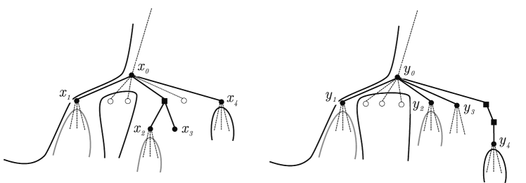
Figure 3: Illustration of the notion of chainable areas of a seed of size 5: $P=\{(x_{0},y_{0}),\ldots,(x_{4},y_{4})\}$ and $CA(P)$ contains $4$ chainable areas each indicated by a different filling pattern.

Appendix: Computing $F(x,y)$ and families of seeds

The cost of the computation of the chainable areas for the border nodes of a seed depends of the nature of this seed. We describe here an efficient algorithm that compute the $F(x,y)$.

Let $P$ be a seed between two trees $Q$ and $T$ and let $B(P)$ the set of pairs of its border nodes. For each node $i$ of $Q$ and $T$ (in fact, only required for the border nodes of $P$), we suppose that we have access to the following informations in $O(1)$:

• $l(i)$: the leftmost leaf of $i$.

• $u(i)$: the node with the highest index such that $r(u(i))=r(i)$ where $r(i)$ is the right most leaf of $i$.

The nodes $u(i)$ are often referred as rightmost roots of the tree.

In Algorithm 3, we use $B$ instead of $B(P)$ and we assume that $B$ is an array of $k$ pairs of nodes on $Q\times T$. For $0\leq i<k$, $B[i]$ represents the $(i+1)^{\text{th}}$ pair of $B$ and $B[i]_{Q}$ is the node $Q$ of this pair and $B[i]_{T}$ is the node of $T$ of this pair.

Algorithm 3 makes use of a stack of pair of nodes called $Stack$. $top(Stack)$ refers to the last element inserted into $Stack$ and similarly to $B$, $top(Stack)_{Q}$ and $top(Stack)_{T}$ are the node of $Q$ and node of $T$ of $top(Stack)$. We write $push(Stack,(x,y))$ to add $(x,y)$ to the top of the stack and $pop(Stack)$ remove the last element of the stack.

The algorithm that computes $F(x,y)$ for all pair of border nodes $(x,y)$ of $P$ is presented in Algorithm 3.

Description of the algorithm.

In the following, a pair of border node of $P$ is called shortly a pair. Pairs are traversed incrementally according to their postfix index. Hence, descendants are visited before parents. Remind that a seed is a valid mapping so ancestral and order relations between borders nodes are respected. Thus, if a border node is a leaf in $P_{Q}$, it is also a leaf in $P_{T}$.

Before each insertion of a new chainable area into $F(x,y)$ we test whether the area is non-empty or not (cf. lines 6, 11, 17, 11 of Algorithm 3).

Let us call the direct descendants of a pair $(x,y)$, the pairs $(x^{\prime},y^{\prime})\in B(P)$ such that $x^{\prime}$ is a descendant of $x$ (resp. $y^{\prime}$ is a descendant of $y$) and there is no border node of $P$ in $Q$ (resp. $T$) between $x^{\prime}$ and $x$ (resp. $y^{\prime}$ and $y$).

Except for the last pair, each time a pair is visited, it is added to the $Stack$ as it is necessarily the direct descendant of a none visited pair. Note that $Stack$ contains pairs sorted incrementally by their postfix index.

Two cases must to be considered: (1) a pair is a pair of leafs in $Q_{P}$, $T_{P}$ ($(x,y)\in L(P)$) and (2) a pair is not a pair of leafs in $Q_{P}$,$T_{P}$ ($(x,y)\not\in L(P)$). Lines 5–8 correspond to the first case and do not require additional explanations.

For the second case, the current pair $(x,y)$ necessarily has direct descendants in $B(P)$. Those descendants have been visited (lower postfix index) and thus are in $Stack$. The chainable area $(a,b,c,d)$ (possible empty) on the right of its rightmost direct descendant $(x^{\prime},y^{\prime})$ ($a>x^{\prime}$ and $c>y^{\prime}$) and the chainable area (possible empty) $(a,b,c,d)$ on the left of its leftmost direct descendant $(x^{\prime\prime},y^{\prime\prime})$ ($b<x^{\prime\prime}$ and $d<y^{\prime\prime}$) require a particular treatment. The possible chainable areas between two direct descendants are considered by the loop on lines 15–19. To compute these chainable areas, the following properties are used in the algorithm: let $(x,y)\in B(P)$

1. Any chainable area $(a,b,c,d)$ of $(x,y)$ are such that $b$ and $d$ are children of $x$ and $y$ and $a$ and $c$ are the leftmost leafs of children of $x$ and $y$.

2. By definition, for chainable areas $(a,b,c,d)$ of $(x,y)$ except the one on the right of its rightmost descendant, $b$ and $d$ are such that $b+1$ and $d+1$ are the leftmost leafs of a direct descendant of $x$ and $y$.

3. For chainable areas $(a,b,c,d)$ of $(x,y)$ except the one on the left of its leftmost descendant, $a$ and $c$ are such that $a-1$ and $c-1$ are children of $x$ and $y$ and are either border nodes or ancestor of border nodes.

As $Stack$ is sorted incrementally, the top of the stack contains the rightmost direct descendant of current pair. Lines 11–12 compute the chainable area on the right of this descendant. Then, loop in lines 15–15 compute the area between the direct descendants using the above properties. Finally, lines 21– 22 compute the chainable area one the left the leftmost direct descendant (that is the last pair $(x^{\prime},y^{\prime})$ in the $Stack$ such that $x^{\prime}\geq l(x)$ and $y^{\prime}\geq l(y)$). Finally, remark that all direct descendant are now out of the $Stack$ and are replaced by the current pair.

The time complexity of this algorithm is $O(|B(P)|)$ as we iterate of all pair and each pair is added only once to the $Stack$.

Note that our algorithm is general as it applies to any sets of seeds as defined in Definition 2. When considering restricted families of seeds, it is possible to design simpler, while still efficient, algorithms to compute the $F(x,y)$ and the chainable areas. For example if one considers only compact seeds, i.e. seeds such that $B(P)=L(P)$ for every seed $P$, then for each border $(x,y)$, $|F(x,y)|=1$ and the computation requires a time linear in the number of seeds. A discussion on the issue of computing chainable areas depending of the combinatorial nature of the considered seeds will be added in a journal version of the current work.

Algorithm 3 $F(x,y)$: compute the $F(x,y)$ for a seed $P$

⬇

1sort $B$ incrementally

2foreach pair $(x,y)$ of $B$ do

3 $F(x,y)=\emptyset$

4for $i$ from $0$ to $k-1$ do

5 if $i=0$ or $B[i-1]_{Q}<l(B[i]_{Q})$ then #$B[i]$ is a pair of leafs in $Q_{P}$ and $T_{P}$

6 if $l(B[i]_{Q})\leq B[i]_{Q}-1$ #$B[i]_{Q}$ is not a leaf in $Q$

7 and $l(B[i]_{T})\leq B[i]_{T}-1$ then #$B[i]_{T}$ is not a leaf in $T$

8 $F(B[i])=(l(B[i]_{Q}),B[i]_{Q}-1,l(B[i]_{T}),B[i]_{T}-1)$

9 else #$B[i]_{Q}$ has at least one descendant in $P$ that is the top of $Stack$

10 # the rightest chainable area of $B[i]$:

11 if $u(top(Stack)_{Q})+1\leq B[i]_{Q}-1$ and $u(top(Stack)_{T})+1\leq B[i]_{T}-1$ then

12 $F(B[i])=(u(top(Stack)_{Q})+1,B[i]_{Q}-1,u(top(Stack)_{T})+1,B[i]_{T}-1)$

13 # the middle chainable areas of $B[i]$:

14 $(x,y)=top(Stack)$; $pop(Stack)$

15 while $Stack$ not empty and $top(Stack)_{Q}\geq l(B[i]_{Q})$ do

16 #insert the area between $(x,y)$ and $top(Stack)_{Q}$ if not empty

17 if $u(top(Stack)_{Q})+1\leq l(x)-1$ and $u(top(Stack)_{T})+1\leq l(y)-1$ then

18 $F(B[i])+=(u(top(Stack)_{Q})+1,l(x)-1,u(top(Stack)_{T})+1,l(y)-1)$

19 $(x,y)=top(Stack)$; $pop(Stack)$

20 # the leftest chainable area of $B[i]$

21 if $l(x)-1\geq l(B[i]_{Q})$ and $l(y)-1\geq l(B[i]_{T})$ then

22 $F(B[i])+=(l(B[i]_{Q}),l(x)-1,l(B[i]_{T}),l(y)-1)$

23 if $i<k-1$ then

24 $push(Stack,())$

References

- [1] S.F. Altschul, W. Gish, W. Miller, E.W. Myers, and D.J. Lipman. Basic local alignment search tool. J. Mol. Biol., 215(3):403–410, 1990.
- [2] S. Aluru, editor. Handbook of Computational Molecular Biology. CRC Press, 2005.
- [3] R. Backofen and S. Will. Local sequence-structure motifs in RNA. J. Bioinform. Comput. Biol., 2(4):681–698, 2004.
- [4] E.D. Demaine, S. Mozes, B. Rossman, and O. Weimann. An optimal decomposition algorithm for tree edit distance. ACM Trans. Algorithms, 6(1):Article 2, 2009.
- [5] P.P. Gardner, J. Daub, J.G. Tate, et al. Rfam: updates to the RNA families database. Nucleic Acids Res., 37(Database issue):D136–D140, 2009.
- [6] D. Gusfield. Algorithms on Strings, Trees and Sequences. Cambridge University Press, 1997.
- [7] S. Heyne, S. Will, M. Beckstette, and R. Backofen. Lightweight comparison of RNAs based on exact sequence-structure matches. Bioinformatics, 25(16):2095–2102, 2009.
- [8] T. Jiang, G. Lin, B. Ma, and K. Zhang. A general edit distance between RNA structures. J. Comput. Biol., 9(2):371–388, 2002.
- [9] D. Joseph, J. Meidanis, and P. Tiwari. Determining DNA sequence similarity using maximum independent set algorithms for interval graphs. In SWAT 1992, volume 621 of LNCS, pp 326–337. 1992.
- [10] D.J. Lipman and W.R. Pearson. Rapid and sensitive protein similarity searches. Science, 227(4693):1435–1441, 1985.
- [11] A. Lozano, R.Y. Pinter, O. Rokhlenko, G. Valiente, and M. Ziv-Ukelson. Seeded tree alignment. IEEE/ACM TCBB, 5(4):503–513, 2008.
- [12] E. Ohlebusch and M.I. Abouelhoda. Handbook of Computational Molecular Biology, chapter Chaining Algorithms and Applications in Comparative Genomics. CRC Press, 2005.
- [13] W.R. Pearson and D.J. Lipman. Improved tools for biological sequence comparison. PNAS, 85(8):2444–2448, 1988.
- [14] B.A. Shapiro and K. Zhang. Comparing multiple RNA secondary structures using tree comparisons. CABIOS, 6:309–318, 1990.
- [15] K. Zhang and D. Shasha. Simple fast algorithms for the editing distance between trees and related problems. SIAM J. Comput., 18(6):1245–1262, 1989.