Modeling broadband X-ray absorption of massive star winds

Abstract

We present a method for computing the net transmission of X-rays emitted by shock-heated plasma distributed throughout a partially optically thick stellar wind from a massive star. We find the transmission by an exact integration of the formal solution, assuming that the emitting plasma and absorbing plasma are mixed at a constant mass ratio above some minimum radius, below which there is assumed to be no emission. This model is more realistic than either the slab absorption associated with a corona at the base of the wind or the exospheric approximation that assumes that all observed X-rays are emitted without attenuation from above the radius of optical depth unity. Our model is implemented in XSPEC as a pre-calculated table that can be coupled to a user-defined table of the wavelength dependent wind opacity. We provide a default wind opacity model that is more representative of real wind opacities than the commonly used neutral interstellar medium (ISM) tabulation. Preliminary modeling of Chandra grating data indicates that the X-ray hardness trend of OB stars with spectral subtype can largely be understood as a wind absorption effect.

1. Introduction

The absorption of soft X-rays by the powerful, radiation-driven winds of OB stars has long been recognized as a significant effect both on the X-rays observed from these stars and on the physical conditions in their winds. The soft X-ray emission observed in OB stars by Einstein and ROSAT implied only modest wind attenuation of the X-rays, and thus ruled out significant coronal emission as a source of the ubiquitous X-ray emission seen in these massive stars (Cassinelli & Olson, 1979; Cassinelli & Swank, 1983; Hillier et al., 1993; MacFarlane et al., 1994). For this and other reasons, the wind-shock paradigm for the production of X-rays in OB stars has become generally accepted (e.g., Owocki et al., 1988; Pauldrach et al., 1994; Feldmeier et al., 1997a, b; Kahn et al., 2001), although many aspects are still poorly understood.

Using X-ray observations to constrain X-ray production mechanisms requires proper account of the absorption of distributed sources of X-ray emission. The amount and wavelength dependence of the wind absorption can be used as a diagnostic of the location/distribution of the shock-heated plasma and of the wind mass-loss rate, especially in terms of its effect on individual line profile shapes (Owocki & Cohen, 2001, hereafter OC01). Even simply deriving an intrinsic X-ray luminosity for energy budget considerations requires correctly modeling the significant attenuation of the emitting X-rays, especially in the dense winds of O supergiants (Hillier et al., 1993; Owocki & Cohen, 1999).

Because the emitting plasma is spatially distributed throughout the absorbing wind, simple prescriptions for the attenuation can be inaccurate. Specifically, the commonly used slab model of absorption, appropriate for an intervening interstellar medium (ISM) cloud where all of the emission originates beyond the absorbing medium, has transmission with an exponential dependence on slab optical depth, and strongly overestimates the amount of attenuation as the wind becomes optically thick. Furthermore, because hydrogen and helium are ionized, models for neutral gas significantly overestimate wind opacity. Unfortunately, due to the lack of easily available tools for incorporating appropriate radiative transfer and opacities, inadequate models, such as those intended for neutral interstellar medium absorption, are routinely applied to account for wind attenuation. This is in spite of the fact that a number of previous works have recognized the necessity for and applied appropriate wind absorption prescriptions (Hillier et al., 1993; Pauldrach et al., 2001; Owocki & Cohen, 2001; Oskinova et al., 2006).

We have developed a method for implementing an exact solution to a realistic model of the radiation transport that can be easily combined with a pre-calculated opacity table to find the wavelength-dependent emergent X-ray flux from a stellar wind. We also provide a reasonable default opacity model that can be used for most OB star winds. Our analysis tool, which we name windtabs, for wind table absorption, can be combined with an independent plasma emission model, such as the Astrophysical Plasma Emission Code (apec) (Smith et al., 2001) that is widely used in fitting stellar X-ray spectra. This can be used to realistically model the low-resolution CCD spectra that are produced in large quantities by surveys of clusters and OB associations with Chandra and XMM-Newton (e.g., Sana et al., 2006; Wang et al., 2008). It can also be used to model grating spectra in detail, and provides a means of disentangling the wind absorption effects from the emission temperature effects that both appear to contribute to the recently discovered trend in the morphology of OB star spectra observed at high resolution with the Chandra gratings (Walborn et al., 2009).

2. Radiation transport model

In this section, we derive an expression for the fraction of X-rays transmitted from a massive star wind as a function of the wavelength-dependent opacity, the mass-loss rate, and the wind velocity law. We make assumptions similar to those made in Owocki & Cohen (2001): we model the wind as a spherically symmetric two-component medium, where a small fraction of the wind is heated to X-ray emitting temperatures ($T_{\mathrm{X}}\sim 1-10\,\mathrm{MK}$), while the bulk of the wind is composed of relatively cool material ($T_{\mathrm{wind}}/T_{\mathrm{eff}}\sim 0.5-1$) that can absorb the X-rays via the bound-free opacity of the moderately ionized metals. We assume that the X-ray emission turns on at some radius $R_{0}>R_{*}$. We also assume that the temperature distribution of the X-ray emitting plasma is the same over the entire emitting volume.

The assumptions we make regarding the distribution of the X-ray emitting plasma are rooted in the available observational evidence, as well as in the results of extensive theoretical simulations. Detailed studies of emission line profiles as well as constraints from forbidden-to-intercombination line ratios in He-like ions support a picture in which X-ray emission starts at $R_{0}\sim 1.5R_{*}$ for all observable ions (Cohen et al., 2006; Leutenegger et al., 2006; Cohen et al., 2010), with a roughly constant filling factor above the onset radius. Numerical simulations have typically found onset radii for strong shocks that are comparable to this (Owocki et al., 1988). Feldmeier et al. (1997b) performed simulations of winds seeded with base perturbations. They have found that clump–clump collisions are important, and that the resulting X-ray emission is distributed primarily below 10 stellar radii. Runacres & Owocki (2002) have also found X-ray emission with onset radii of order 1.5 stellar radii and extending out to large radii. However, the results for the onset radius are also sensitive to the treatment of the scattered radiation field (Owocki & Puls, 1996; Owocki, 2009).

The observed X-ray luminosity as a function of wavelength is given by

$$L_{\lambda}=4\pi\,\int\,dV\,\eta_{\lambda}(r)\,e^{-\tau(r,\mu,\lambda)}\,,$$ (1)

where $\eta_{\lambda}(r)$ is the X-ray emissivity, and $\tau(r,\mu,\lambda)$ is the continuum optical depth of the dominant cool component along a ray from the emitting volume element to the observer.

The optical depth can be derived as in Owocki & Cohen (2001) for a smooth wind. It is given by the integral

$$\tau(p,z,\lambda)=\int_{z}^{\infty}\,dz^{\prime}\,\kappa(\lambda)\,\rho(r^{\prime})\,.$$ (2)

Here $p$ and $z$ are ray coordinates, with impact parameter $p=\sqrt{1-\mu^{2}}\,r$ and distance along the ray $z=\mu\,r$, where $\mu$ is the direction cosine to the observer at local radius $r$. $\kappa(\lambda)$ is the atomic opacity of the wind, and $\rho(r)$ is the density of the wind. Using the continuity equation, $\rho(r)=\dot{M}/4\pi r^{2}v(r)$, where $\dot{M}$ is the stellar mass loss rate, and defining the characteristic wind optical depth,

$$\tau_{*}\equiv\frac{\kappa(\lambda)\,\dot{M}}{4\pi R_{*}v_{\infty}}\,,$$ (3)

we can write

$$\tau(p,z)=\tau_{*}\,t(p,z)\,,$$ (4)

where

$$t(p,z)\equiv\int_{z}^{\infty}\,\frac{R_{*}dz^{\prime}}{r^{\prime 2}w(r^{\prime})}$$ (5)

is a dimensionless integral that depends purely on the ray geometry. Here, $R_{*}$ is the stellar radius, $v_{\infty}$ is the wind terminal velocity, and $w(r)\equiv v(r)/v_{\infty}$ is the scaled wind velocity. Note that we have assumed that $\kappa(\lambda)$ is constant throughout the wind; we further discuss this assumption in Section 3. We take the velocity to follow a beta law: $v=v_{\infty}(1-R_{*}/r)^{\beta}$. We also take $\beta=1$ in this paper as a good approximation for many O star winds; however, evaluation for general values of $\beta$ is not difficult.

The emissivity is assumed to scale with density squared, as in Owocki & Cohen (2001). We ignore the Doppler shift of the emitted X-rays and write

$$\eta_{\lambda}(r>R_{0})=\eta_{\lambda,0}\frac{\rho^{2}(r)}{\rho^{2}_{0}}\,.$$ (6)

This expression gives the correct radial dependence for the total line strength, but discards information about the profile shape. This is a justified approximation in calculating the broadband X-ray transmission of the wind. Here we assume that X-ray emission begins at a minimum radius $R_{0}$, with $\rho_{0}\equiv\rho(R_{0})$ and $\eta_{\lambda,0}\equiv\eta_{\lambda}(R_{0})$. In this paper, we will assume that the X-ray filling factor is constant with radius; it is trivial to add a power-law radial dependence, as in OC01. We also assume that X-ray emissivity follows the same radial distribution at all observable wavelengths.

The model described in the preceding paragraphs is illustrated in Figures 1 and 2. The model emissivity and transmission are visualized separately in Figure 1, and together in the left panel of Figure 2. The right panel of Figure 2 gives the net transmission for the exospheric approximation for comparison, which we discuss at more length below.

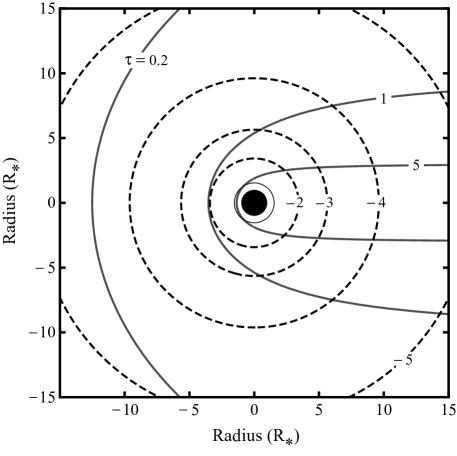
Figure 1.— This diagram shows the X-ray emission and absorption properties of a model stellar wind. The observer is on the left. The black disk denotes the star, and the thin black line shows the onset radius for X-ray emission (1.5 $R_{*}$ in this case). Contours of constant X-ray emissivity (proportional to density squared) are shown with dashed lines at intervals of an order of magnitude in differential emissivity. The absolute scale is normalized to the maximum emissivity at the onset radius of X-ray emission. Contours of constant continuum optical depth calculated for $\tau_{*}=3$ are shown with solid lines.

Figure 2.— Left panel is the same as Figure 1, but plotting the net emissivity (product of intrinsic emissivity times transmission, including occultation by the stellar core) instead of the intrinsic emissivity; this net emissivity has been renormalized so that the point of maximum net emissivity has a value of unity. The right panel shows the same plot in the exospheric approximation, where the gray zone is inside the radius of (radial) optical depth unity and thus does not contribute to the observed X-ray flux.

Using Equations (1)–(6), we can calculate the transmission of the wind as a function of $\tau_{*}$. The transmission is simply the observed flux (Equation (1)) divided by the unattenuated flux, which can be found by setting $\tau_{*}=0$ in the same equation:

$$T(\tau_{*})\equiv\frac{L_{\lambda}(\tau_{*})}{L_{\lambda}(0)}=\frac{\int dV\,\rho^{2}\,e^{-\tau}}{\int dV\rho^{2}}\,.$$ (7)

To account for the attenuation in the numerator, it is convenient to define an angle-averaged transmission from each radius $r$.

$$\overline{T}(r,\tau_{*})\equiv\frac{1}{2}\int^{1}_{-\mu_{*}}d\mu\,e^{-\tau_{*}t(r,\mu)}\,,$$ (8)

where

$$\mu_{*}=\sqrt{1-\frac{R_{*}^{2}}{r^{2}}}\,$$ (9)

gives the $\mu$ coordinate of occultation by the the stellar core. Some X-rays are obscured by the stellar core even when the wind is transparent:

$$\overline{T}_{0}(r)\equiv\overline{T}(r,0)=\frac{1}{2}(1+\mu_{*})\,.$$ (10)

Integrating over shells at all radii, the net transmission is thus

$$T(\tau_{*})=\frac{\int_{R_{0}}^{\infty}\,dr\,r^{2}\,\rho^{2}(r)\,\overline{T}(r,\tau_{*})}{\int_{R_{0}}^{\infty}\,dr\,r^{2}\,\rho^{2}(r)}\,.$$ (11)

We can further evaluate this expression by substituting the continuity equation, and by defining the inverse radial coordinate $u\equiv R_{*}/r$:

$$T(\tau_{*})=\frac{\int_{0}^{u_{0}}\,du\,w^{-2}(u)\overline{T}(u,\tau_{*})}{\int_{0}^{u_{0}}\,du\,w^{-2}(u)}\,.$$ (12)

Figure 3 shows the angle-averaged transmission $\bar{T}(u)$ for selected values of $\tau_{*}$. Figure 4 shows the following quantity:

$$\frac{L_{\lambda}(u,\tau_{*})}{L_{\lambda}(u_{0},\tau_{*})}=\frac{\int^{u}_{0}du^{\prime}w^{-2}(u^{\prime})\overline{T}(u^{\prime},\tau_{*})}{\int^{u_{0}}_{0}du^{\prime}w^{-2}(u^{\prime})\overline{T}(u^{\prime},\tau_{*})}$$ (13)

This can be thought of as the cumulative distribution of observed X-ray emission, starting from $u=0$ ($R=\infty$) and integrating in to $u=u_{0}$. Together, Figures 3 and 4 show the relative importance of transmission and emission as a function of radius in stellar winds. For the entire range of interest in $\tau_{*}$, essentially all of the wind down to $u_{0}$ contributes to the observed X-ray flux.

Figure 5 shows $T(\tau_{*})$ for this model, along with comparisons to two other absorption prescriptions: a simple intervening absorber, $T=e^{-\tau}$, appropriate for a coronal slab model, e.g., as implemented in the XSPEC models wabs or tbabs; and an exospheric approximation (e.g. Owocki & Cohen, 1999), where $T=0$ below the radius of optical depth unity, and $T=1$ everywhere above it:

$$T_{\mathrm{exo}}(\tau_{*})=\frac{\int_{0}^{u_{x}}\,du\,w^{-2}(u)}{\int_{0}^{u_{0}}\,du\,w^{-2}(u)}\,,$$ (14)

where $u_{x}\equiv\min(u_{1}(\tau_{*}),u_{0})$. The inverse radial coordinate of optical depth unity is given by evaluating the optical depth integral (Equation (5)) along a radial ray ($p=0$, $z=r$), with the result

$$u_{1}(\tau_{*})=1-e^{-1/\tau_{*}}\,,$$ (15)

for $\beta=1$. Note that in Figures 3-5, we have used $\beta=1$ and $R_{0}=1.5R_{*}$. We stress that Equation (14) is simply the consequence of using a step function for the angle-averaged transmission $\overline{T}$ in Equation (12), rather than the more realistic expression given in Equation (8).

The transmission of our model falls off much more gradually than $e^{-\tau}$ (Figure 5), but it is also more accurate than the exospheric approximation, especially at moderate optical depth. The exospheric approximation has the correct asymptotic behavior for large values of $\tau_{*}$, but overestimates the transmission by a fixed factor. The exospheric transmission at large $\tau_{*}$ can be brought into agreement with windtabs by multiplying the exospheric $\tau_{*}$ by three.

It would be possible to generalize the radiation transport model described in this section to include porosity by introducing an appropriate definition of effective opacity, as in Oskinova et al. (2006) or Owocki & Cohen (2006). However, a specific implementation of this and discussion of its consequences is left to a future study.

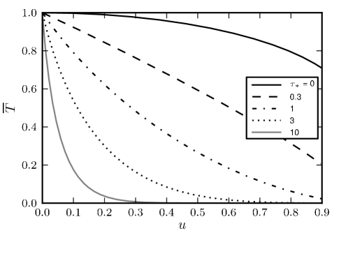
Figure 3.— Angle averaged transmission $\overline{T}$ as a function of shell inverse radial coordinate $u=R_{*}/r$, with different curves for different characteristic wind optical depths $\tau_{*}$. The equivalent plot in the exospheric approximation would be a step function at $u_{1}$, the inverse radial coordinate of optical depth unity. Note that the transmission is less than unity even for $\tau_{*}=0$ due to occultation by the stellar core.

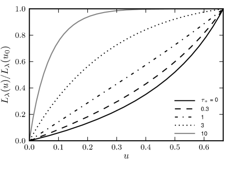
Figure 4.— Fraction of X-ray emission originating from outside inverse radius $u$, normalized to total X-ray emission integrated to $u_{0}=2/3$. For all but the very optically thick case of $\tau_{*}=10$, the emission comes from a wide range in $u$.

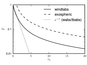
Figure 5.— Comparison of transmission of three different models: coronal slab ($e^{-\tau}$), exospheric, and more realistic wind model (windtabs). The fixed parameters are $\beta=1$, $R_{0}=1.5$.

3. Opacity model

To determine the wind transmission as a function of wavelength, we need to account for the wavelength dependence of the optical depth through the opacity, which we write as

$$\tau_{*}(\lambda)=\kappa(\lambda)\Sigma_{*}\,,$$ (16)

where

$$\Sigma_{*}\equiv\frac{\dot{M}}{4\pi R_{*}v_{\infty}}$$ (17)

is the characteristic mass column density of the wind (in $\mathrm{g}\,\mathrm{cm}^{-2}$).

The continuum opacity of a stellar wind in the X-ray band can be calculated by summing the contributions of each constituent species. Thus, we must know the atomic cross-sections, ionization fractions, and elemental abundances. Of these three, the cross sections are known to sufficient accuracy (e.g. Verner & Yakovlev, 1995); the ionization balance may contribute some uncertainty in the calculation of the opacity, but is usually not the dominant source of error; and uncertainties in the elemental abundances are typically the most important.

The opacity due to photoionization of a given shell of any individual species scales approximately as $\kappa_{i}(\lambda)\propto\lambda^{3}$ above the threshold energy $E_{\mathrm{th}}$ of the shell. Because multiple species are usually important for the X-ray opacity of astrophysical gas, the run of opacity with wavelength has a characteristic sawtooth shape, with individual teeth at the ionization threshold energies of dominant ionization stages of abundant elements.

O star winds are photoionized, with H and He fully stripped (although He may recombine in some dense winds; see below), and most other elements mainly in charge states +3 and +4. Thus, the opacity of stellar winds in the range 1 Å $<\lambda<$ 40 Å is dominated by K-shell absorption in C, N, and O, since they are the most abundant elements. Significant contributions from K-shell absorption in Ne, Mg, and Si are also present, as well as Fe L-shell absorption.

The opacity of adjacent ionization stages of the same element are usually comparable, with the exception that the photoionization threshold energy is shifted. The effect of a moderate shift in ionization balance on the opacity is relatively minor, since none of the strong X-ray emission lines observed from O star winds falls between the threshold energies of adjacent stages of abundant ions. However, the difference in threshold energies, and hence the broadband absorption, between neutral and wind material is significant.

Therefore, while it is important to use an appropriate model for the wind ionization, it is sufficient for many applications to use a single approximate ionization balance to model all O star winds. This is true even though the ionization balance can vary to some extent with radius, and also is different in different stars.

If it is desired to model the opacity of a particular star, it is possible to construct a detailed model opacity for a stellar wind by using the output of a radiative transfer model such as CMFGEN (Hillier et al., 1993; Hillier & Miller, 1998; Cohen et al., 2010, J. Zsargó et al., in preparation).

To illustrate the importance of various assumptions in opacity modeling, Figures 6 and 7 compare several model opacities. Figure 6 compares neutral interstellar medium opacity and a simple model for the opacity of a stellar wind. Both assume solar abundances (Asplund et al., 2009). In the wind model we assume an ionization balance with hydrogen and helium fully stripped, oxygen and nitrogen in the +3 charge state, and all other elements in the +4 charge state. This is a good approximation to the ionization balance in a typical O star wind, which is set by photoionization from the photospheric UV field. The model wind opacity is much lower than the model ISM opacity, especially at long wavelengths, mainly due to the ionization of hydrogen and helium. The shift in ionization threshold energies due to the presence of more highly ionized species is also clear.

Figure 7 shows three stellar wind model opacities, and thereby illustrates the relative importance of two effects on the opacity: the elemental abundances, and the ionization balance. The solid line gives the same solar abundance wind model described in the previous paragraph, while the dashed and dotted lines give models particular to $\zeta$ Pup, using non-solar abundances specific to the star derived from detailed CMFGEN modeling (J.-C. Bouret et al., in preparation). The dashed line gives the actual opacity at $\sim 2R_{*}$ from this CMFGEN model, while the dotted line uses the simplified ionization structure of the solar abundance wind opacity model. The fact that the realistic CMFGEN $\zeta$ Pup model and the simplified version are so similar indicates that a simple ionization balance is typically adequate to describe wind opacity in many cases, as long as the dominant ionization stages are relatively accurate. On the other hand, the difference between the $\zeta$ Pup models and the solar abundance model shows that the opacity model depends strongly on the abundances of the most common elements other than H and He (typically C, N, and O). Note that the Bouret et al. abundances for $\zeta$ Pup are both non-solar in the ratio of CNO and also have sub-solar metallicity; it is the sub-solar metallicity that accounts for the lower opacity of the $\zeta$ Pup models at short wavelengths compared to the solar abundance model.

We have made one important simplification in our modeling: in Equation (4), and throughout this section, we have assumed that the opacity is independent of radius. As shown in Figure 7, moderate changes in wind ionization do not strongly affect the opacity, so in most cases this is a justified approximation. The important exception is the ionization of helium; in sufficiently dense winds, He⁺⁺ may recombine to He⁺ in the outer part of the wind, which greatly increases the opacity, especially at long wavelengths (Pauldrach, 1987; Hillier et al., 1993). As long as the change in ionization occurs sufficiently far out in the wind, geometrical effects as described in Section 2 are not important, and the absorption due to He⁺ can be treated as an additional slab between the X-ray emitting regions and the observer, i.e., using $T=e^{-\tau}$.

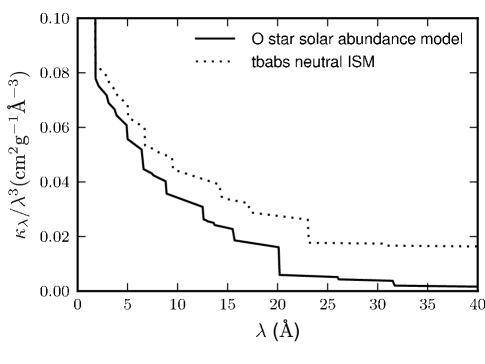
Figure 6.— Comparison of a neutral interstellar absorption model (including dust grains), tbabs (Wilms et al., 2000); and an O star wind model with an assumed simple ionization structure. The opacity $\kappa(\lambda)$ is scaled with $\lambda^{3}$ to allow a better comparison of the two models at short wavelengths. Both models use solar abundances (Asplund et al., 2009). Note that even below the O³⁺ edge near 20 Å, the wind opacity model is still about 40% lower than the ISM model, mainly due to the ionization of H and He in the wind model.

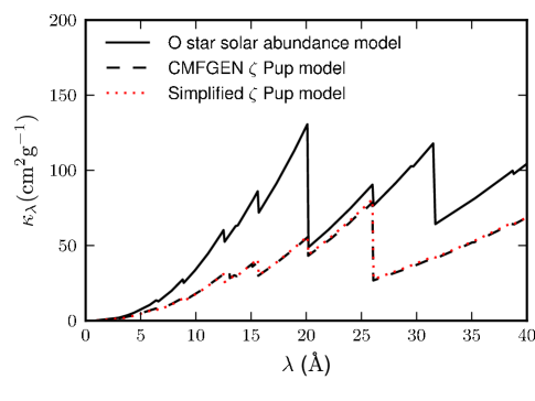
Figure 7.— Comparison of three different model O star wind opacities: the solar abundance O star wind model (with assumed simple ionization structure) shown in Figure 6 (solid); a CMFGEN model appropriate for $\zeta$ Pup (dashed) using the abundances of J.-C. Bouret et al. (in preparation); and a simplified version of this CMFGEN model (dotted; red in the electronic version) where the ionization balance is the same as in the solar abundance model. Note that the Bouret et al. abundances for $\zeta$ Pup are subsolar as well as having altered CNO abundance ratios.

4. Model Implementation

The numerical evaluation of Equation (12) is not prohibitively expensive, but it is typically not fast enough to allow its use in an automated spectral fitting routine, such as that in XSPEC12 (Arnaud, 1996) or ISIS (Houck & Denicola, 2000). It is thus preferable to compute the transmission on a grid in $\tau_{*}$ for a given set of wind parameters.

Given a tabulation of the model wind opacity, as described in Section 3, in addition to the tabulation of $T(\tau_{*})$, one may then calculate the transmission as a function of wavelength, $T(\lambda)$, with only one free parameter, the characteristic wind mass column density $\Sigma_{*}$. This parameter is analogous to the neutral hydrogen column density in a slab absorption model such as the XSPEC wabs or tbabs ISM absorption models (which are also sometimes used to approximate wind absorption).

We have implemented this as a local model for XSPEC 12. A user can calculate $T(\tau_{*})$ for a given set of parameters (i.e., $\beta$, $R_{0}$), with the results stored in a FITS table. These implicit model parameters may be varied by computing additional tables of $T(\tau_{*})$ for each set of parameter values. However, the absorption model is not very sensitive to these parameters over the range typically inferred for winds of massive stars. The calculation of $T(\tau_{*})$ is controlled by a simple python script, and computation of a table for a given set of parameters can be accomplished in several seconds on a modern workstation. The model opacity must also be supplied as a FITS file; different model opacities may be swapped in at run time. When windtabs is used in a spectral fitting program, model transmission is calculated as a function of energy or wavelength using the supplied FITS tables and the one free model parameter, $\Sigma_{*}$.

The elemental abundances, which enter into the transmission through their effect on the opacity, cannot be varied as fit parameters in our model. This is a choice we have made in the model implementation, both for computational ease and simplicity of user interface, and because there is not enough information in X-ray spectra to constrain elemental abundances through modeling of absorption of X-ray emission alone. Abundances should be inferred by other means, e.g., from global fits to UV and optical spectra, or from fits to X-ray emission line strengths. These abundances can be used to compute a new opacity table for a given star.

Figure 8 gives the model transmission for windtabs using three different values of $\Sigma_{*}$, and using our standard O star wind opacity model. For comparison, this figure also shows the transmission for the neutral absorption model tbabs for comparable mass column densities $\Sigma$. Note that $\Sigma$ refers simply to a slab mass column density, while $\Sigma_{*}$ refers to a characteristic mass column density in the context of a stellar wind (see Equation (17)).

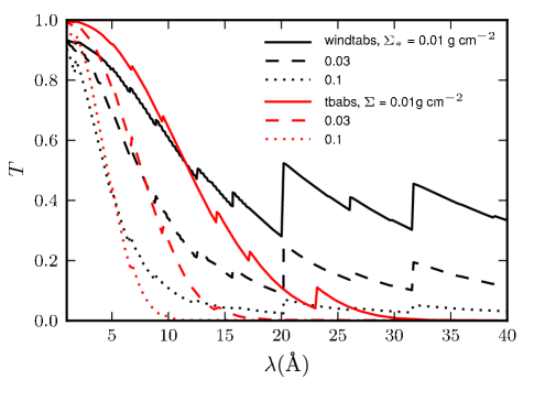
Figure 8.— Transmission as a function of wavelength for ionized wind absorption model (windtabs, black) and for neutral slab absorption (tbabs, gray; red in the electronic version). Three values of absorbing column are given; for windtabs, the degree of absorption is specified by the characteristic mass column density $\Sigma_{*}$, while for tbabs it is given simply by the mass column $\Sigma$.

5. Discussion

5.1. Advantages of windtabs over exospheric or exponential attenuation

The exact method we have presented here for modeling the X-ray radiative transfer for a distributed source embedded within a stellar wind is crucial for analyzing the X-ray emission observed from O stars. Compared to the exponential, neutral slab absorption (excess over ISM) model that is usually employed, the windtabs model accurately reproduces the much more gradual decrease in transmission with increasing wind column density and opacity. This can be seen in Figure 8, where the exponential transmission model shows an unrealistically sudden decrease in transmission when the wind becomes optically thick.

Because the opacity of the bulk wind is a relatively strong function of wavelength, the inaccuracy of the exponential transmission model will lead to errors in the broadband spectral energy distribution of a model applied to individual O stars, leading to misinterpretations of the associated emission model components. This appears to be the case in the study of Chandra grating spectra in Zhekov & Palla (2007), which invokes excess exponential, neutral ISM absorption to account for the assumed wind attenuation. Most likely because the exponential transmission radiation transport model, and also the neutral ISM opacity model, significantly overestimates the degree of attenuation, these authors find absorption beyond the ISM column for only one star, even though some additional wind attenuation is expected for most of the stars in their sample. Additionally, although the authors do not comment on it, their determination of elemental abundances for each of the stars shows a consistent trend of abundance correlated with the wavelength of the dominant line or lines from each element. Such an effect would be expected if the wavelength-dependent wind attenuation is not accurately accounted for.

It has long been noted that the exponential attenuation treatment is not well suited to modeling OB star X-rays. Hillier et al. (1993) used an exact treatment in their modeling of $\zeta$ Pup, discarding the possibility of a coronal model on the basis of the strong soft observed X-ray flux of $\zeta$ Pup, together with its relatively high mass-loss rate. Cohen et al. (1996) showed that an exospheric treatment, rather than an exponential treatment, is important for understanding the observed EUV and soft X-ray emission from the early B giant, $\epsilon$ CMa. The exospheric approximation was used by Owocki & Cohen (1999) to model the effect of wind attenuation of X-rays in order to explain the observed $L_{x}/L_{\mathrm{bol}}\sim 10^{-7}$ relationship and its breakdown in the early B spectral range where hot star winds become optically thin to X-rays. An exospheric treatment was also used by Oskinova et al. (2001) to analyze the variability of X-rays from optically thick WR winds. And the exospheric framework forms the basis for the “optical depth unity” relationship for X-rays in O stars, where the forbidden-to-intercombination line ratios of helium-like ions are claimed to imply formation radii that track the optical depth unity radius as a function of X-ray wavelength (Waldron & Cassinelli, 2007).

However, the exospheric treatment underestimates the attenuation of the wind. If data need to be analyzed with a high degree of accuracy, then a more realistic treatment of X-ray radiation transport through the wind must be used; one that takes the inherently non-spherically symmetric nature of the problem into account. This is especially true when the location of the X-ray emission emerging from the wind is important, as with the interpretation of $f/i$ ratios. As Figure 2 shows, the relative contribution of the emergent X-ray flux from different wind regions is incorrectly estimated in the exospheric approach, and as Figure 4 shows, the emergent flux has significant contributions from a wide range of radii. In fact, a number of previous works have implemented accurate X-ray radiative transfer prescriptions (e.g., Pauldrach et al., 2001; Owocki & Cohen, 2001; Oskinova et al., 2006); however, none of these works provide an implementation that is available for use in other contexts.

The windtabs model we have introduced here is not only more accurate in terms of the radiation transport than slab or exopheric treatments, but it has two additional advantages that recommend its adoption for routine X-ray data analysis and modeling of O stars. First, it is easy to use and has only a single free parameter, the characteristic mass column density $\Sigma_{*}$, from which a mass-loss rate can be readily extracted. And second, it incorporates a default wind opacity model that is significantly different from, and much more accurate than, the neutral ISM opacity models that are usually used. Additionally, alternate user-calculated opacity models are easy to incorporate.

5.2. Implications for trends in X-ray hardness with spectral type

One application of windtabs to the interpretation of X-ray spectral data is for the analysis of the X-ray spectral hardness trend versus optical spectral subtype recently noted in Chandra grating spectra by Walborn et al. (2009). They report “the progressive weakening of the higher ionization relative to the lower ionization X-ray lines with advancing spectral type, and the similarly decreasing intensity ratios of the H-like to He-like lines of the $\alpha$ ions.” The correlation of the overall X-ray spectral hardness with spectral subtype described by Walborn et al. appear to be a direct result of wavelength dependent absorption effects. A detailed analysis is in preparation, but here we show a single suite of models in which the only variable parameter is the characteristic wind column density, $\Sigma_{*}$. A single emission model, combined with windtabs attenuation, reproduces the observed broadband trend quite well.

Figure 9 shows X-ray grating spectra for seven O giants and supergiants in the left-hand column, with the earliest spectral subtype (O3.5) on the top, and the latest (B0) on the bottom, as in Walborn et al. (2009). The later spectral subtypes clearly have more soft X-ray emission, although the earlier subtypes still have non-negligible long-wavelength ($\lambda\gtrsim 15$ Å) emission. In the middle column we show a four-temperature apec (Smith et al., 2001) thermal equilibrium emission model. We have chosen $kT$ = 0.1, 0.2, 0.4, and 0.6 keV; the first three components having equal emission measures and the hottest one having half the emission measure of the others. The same apec model is used for all seven stars (with variable overall normalization) and is multiplied by a windtabs model and a tbabs model (for neutral ISM attenuation). The column density of the tbabs model is fixed at the interstellar value taken from Fruscione et al. (1994), with the exception of HD 150136, for which we inferred the ISM column density from E(B-V) (Maíz-Apellániz et al., 2004; Martins & Plez, 2006; Vuong et al., 2003). The characteristic mass column density $\Sigma_{*}$ in windtabs is fixed at a value computed from the “cooking formula” theoretical mass-loss rate computed by Vink et al. (2001), using the measured terminal velocity of Haser (1995) and the modeled radii of Martins et al. (2005). The standard solar abundance wind opacity model (solid line in Figure 7) was used in windtabs, and the apec model abundances were set to solar. There are no free parameters in these models, and the temperature distribution has not even been significantly optimized to match the data. The adopted parameters are listed in Table 1.

Table 1Adopted Stellar Parameters

Star	Spectral Type	$N_{\mathrm{H}}$	$\Sigma_{*}$	$N_{*}$
HD 150136	O3.5 If* + O6V	0.76	0.073	3.6
$\zeta$ Pup	O4 I(n)f	0.01	0.160	7.2
$\xi$ Per	O7.5 III(n)((f))	0.115	0.017	0.76
$\tau$ CMa	O9 II	0.056	0.013	0.58
$\delta$ Ori	O9.5 II + B0.5 III	0.015	0.011	0.49
$\zeta$ Ori	O9.7 Ib	0.03	0.019	0.85
$\epsilon$ Ori	B0 Ia	0.03	0.020	0.89

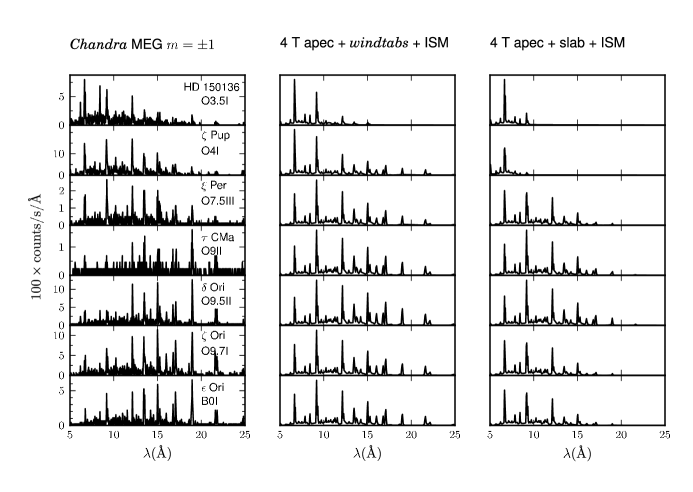
Figure 9.— Left column: a sequence of Chandra spectra of O giants and supergiants from Walborn et al. (2009); middle column: multi-temperature thermal emission model with windtabs wind absorption model; right column: same model as middle column, but with tbabs neutral slab absorption model.

As the middle column of Figure 9 shows, the simple, universal emission model reproduces the broadband trend very well. Trends in individual line ratios generally cannot be reproduced only by accounting for the varying attenuation, as pointed out by Walborn et al. (2009), but note that the Ne IX (13.5 Å) to Ne X (12.1 Å) ratio does indeed vary due only to differential attenuation among the earliest spectral subtypes. The right-hand column in Figure 9 shows the same emission and ISM attenuation models as in the middle column, but with excess exponential (neutral ISM) attenuation accounting for the wind absorption, again according to the wind column densities expected from the adopted mass-loss rates, radii, and terminal velocities. The exponential attenuation trend seen in the right-hand column is too strong for the earliest spectral subtypes and too weak for the latest ones, where the different ISM column densities actually dominate the trend.

The contrast between the windtabs and exponential models is quite stark, and indicates that the more realistic models should generally be used when analyzing X-ray spectra, both high-resolution and broadband. It is also impressive how much of the observed spectral hardness trend is explained by wind attenuation, in the context of a realistic model. Not only do quantitative analyses of the suggested line ratio trends have to be evaluated, but a global spectral modeling that allows for both emission temperature variations and wind attenuation variations should be undertaken in order to disentangle the relative contributions of trends in emission and absorption to the overall, observed trend in the spectral energy distributions.

6. Conclusions

We have presented an exact solution to the radiation transport of X-rays through a spherically symmetric, partially optically thick O star wind, and shown that it differs significantly from the commonly used slab absorption and exospheric models. Specifically, the transmission falls off much more gradually as a function of fiducial optical depth in the windtabs model as compared to the exponential model, leading to more accurate assessments of wind column densities and mass-loss rates from fitting X-ray spectra. As one example of the utility of windtabs, we have shown that when this more accurate model is employed, differential wind absorption can explain most of the observed trend in OB star X-ray spectral hardness with spectral subtype, and even may explain some of the line ratio trend.

The windtabs model has been implemented as a custom model in XSPEC, and is as easy to use as the various ISM absorption models, having only one free parameter. In addition to the significantly improved accuracy of the radiation transport, windtabs has several other advantages. It incorporates a default opacity model much more appropriate to stellar winds than the neutral element opacity model used in ISM attenuation codes. Users can easily substitute their own custom-computed opacity models. And the fitted mass column density parameter for windtabs allows for the user to extract a mass-loss rate directly from their fitting of X-ray spectra of OB stars.

References

- Arnaud (1996) Arnaud, K. A. 1996, in ASP Conf. Ser., Vol. 101, Astronomical Data Analysis Software and Systems V, ed. G. H. Jacoby & J. Barnes, (San Francisco, CA: ASP), 17
- Asplund et al. (2009) Asplund, M., Grevesse, N., Sauval, A. J., & Scott, P. 2009, ARA&A, 47, 481
- Cassinelli & Olson (1979) Cassinelli, J. P. & Olson, G. L. 1979, ApJ, 229, 304
- Cassinelli & Swank (1983) Cassinelli, J. P. & Swank, J. H. 1983, ApJ, 271, 681
- Cohen et al. (1996) Cohen, D. H., Cooper, R. G., MacFarlane, J. J., Owocki, S. P., Cassinelli, J. P., & Wang, P. 1996, ApJ, 460, 506
- Cohen et al. (2006) Cohen, D. H., Leutenegger, M. A., Grizzard, K. T., Reed, C. L., Kramer, R. H., & Owocki, S. P. 2006, MNRAS, 368, 1905
- Cohen et al. (2010) Cohen, D. H., Leutenegger, M. A., Wollman, E. E., Zsargó, J., Hillier, D. J., Townsend, R. H. D., & Owocki, S. P. 2010, MNRAS, 405, 2391
- Feldmeier et al. (1997a) Feldmeier, A., Kudritzki, R.-P., Palsa, R., Pauldrach, A. W. A., & Puls, J. 1997a, A&A, 320, 899
- Feldmeier et al. (1997b) Feldmeier, A., Puls, J., & Pauldrach, A. W. A. 1997b, A&A, 322, 878
- Fruscione et al. (1994) Fruscione, A., Hawkins, I., Jelinsky, P., & Wiercigroch, A. 1994, ApJS, 94, 127
- Haser (1995) Haser, S. M. 1995, PhD thesis, Universitäts-Sternwarte der Ludwig-Maximillian Universität, München, (1995)
- Hillier et al. (1993) Hillier, D. J., Kudritzki, R. P., Pauldrach, A. W., Baade, D., Cassinelli, J. P., Puls, J., & Schmitt, J. H. M. M. 1993, A&A, 276, 117
- Hillier & Miller (1998) Hillier, D. J. & Miller, D. L. 1998, ApJ, 496, 407
- Houck & Denicola (2000) Houck, J. C. & Denicola, L. A. 2000, in ASP Conf. Ser., Vol. 216, Astronomical Data Analysis Software and Systems IX, ed. N. Manset, C. Veillet, & D. Crabtree, (San Francisco, CA: ASP), 591
- Kahn et al. (2001) Kahn, S. M., Leutenegger, M. A., Cottam, J., Rauw, G., Vreux, J.-M., den Boggende, A. J. F., Mewe, R., & Güdel, M. 2001, A&A, 365, L312
- Leutenegger et al. (2006) Leutenegger, M. A., Paerels, F. B. S., Kahn, S. M., & Cohen, D. H. 2006, ApJ, 650, 1096
- MacFarlane et al. (1994) MacFarlane, J. J., Cohen, D. H., & Wang, P. 1994, ApJ, 437, 351
- Maíz-Apellániz et al. (2004) Maíz-Apellániz, J., Walborn, N. R., Galué, H. Á., & Wei, L. H. 2004, ApJS, 151, 103
- Martins & Plez (2006) Martins, F. & Plez, B. 2006, A&A, 457, 637
- Martins et al. (2005) Martins, F., Schaerer, D., & Hillier, D. J. 2005, A&A, 436, 1049
- Oskinova et al. (2006) Oskinova, L. M., Feldmeier, A., & Hamann, W.-R. 2006, MNRAS, 372, 313
- Oskinova et al. (2001) Oskinova, L. M., Ignace, R., Brown, J. C., & Cassinelli, J. P. 2001, A&A, 373, 1009
- Owocki (2009) Owocki, S. 2009, in AIP Conf. Ser., Vol. 1171, Radiation Hydrodynamics of Line-Driven Winds, ed. I. Hubeny, J. M. Stone, K. MacGregor, & K. Werner, (Melville, NY: AIP), 173
- Owocki et al. (1988) Owocki, S. P., Castor, J. I., & Rybicki, G. B. 1988, ApJ, 335, 914
- Owocki & Cohen (1999) Owocki, S. P. & Cohen, D. H. 1999, ApJ, 520, 833
- Owocki & Cohen (2001) —. 2001, ApJ, 559, 1108
- Owocki & Cohen (2006) —. 2006, ApJ, 648, 565
- Owocki & Puls (1996) Owocki, S. P. & Puls, J. 1996, ApJ, 462, 894
- Pauldrach (1987) Pauldrach, A. 1987, A&A, 183, 295
- Pauldrach et al. (2001) Pauldrach, A. W. A., Hoffmann, T. L., & Lennon, M. 2001, A&A, 375, 161
- Pauldrach et al. (1994) Pauldrach, A. W. A., Kudritzki, R. P., Puls, J., Butler, K., & Hunsinger, J. 1994, A&A, 283, 525
- Runacres & Owocki (2002) Runacres, M. C. & Owocki, S. P. 2002, A&A, 381, 1015
- Sana et al. (2006) Sana, H., Rauw, G., Nazé, Y., Gosset, E., & Vreux, J. 2006, MNRAS, 372, 661
- Smith et al. (2001) Smith, R. K., Brickhouse, N. S., Liedahl, D. A., & Raymond, J. C. 2001, ApJ, 556, L91
- Verner & Yakovlev (1995) Verner, D. A. & Yakovlev, D. G. 1995, A&AS, 109, 125
- Vink et al. (2001) Vink, J. S., de Koter, A., & Lamers, H. J. G. L. M. 2001, A&A, 369, 574
- Vuong et al. (2003) Vuong, M. H., Montmerle, T., Grosso, N., Feigelson, E. D., Verstraete, L., & Ozawa, H. 2003, A&A, 408, 581
- Walborn et al. (2009) Walborn, N. R., Nichols, J. S., & Waldron, W. L. 2009, ApJ, 703, 633
- Waldron & Cassinelli (2007) Waldron, W. L. & Cassinelli, J. P. 2007, ApJ, 668, 456
- Wang et al. (2008) Wang, J., Townsley, L. K., Feigelson, E. D., Broos, P. S., Getman, K. V., Román-Zúñiga, C. G., & Lada, E. 2008, ApJ, 675, 464
- Wilms et al. (2000) Wilms, J., Allen, A., & McCray, R. 2000, ApJ, 542, 914
- Zhekov & Palla (2007) Zhekov, S. A. & Palla, F. 2007, MNRAS, 382, 1124