Spin-charge-density wave in a squircle-like Fermi surface for ultracold atoms

Abstract

We derive and discuss an experimentally realistic model describing ultracold atoms in an optical lattice including a commensurate, but staggered, Zeeman field. The resulting band structure is quite exotic; fermions in the third band have an unusual rounded picture-frame Fermi surface (essentially two concentric squircles), leading to imperfect nesting. We develop a generalized ${\rm SO}(3,1)\times{\rm SO}(3,1)$ theory describing the spin and charge degrees of freedom simultaneously, and show that the system can develop a coupled spin-charge-density wave order. This ordering is absent in studies of the Hubbard model that treat spin and charge density separately.

Introduction Ultracold atoms in optical lattices have recently emerged as a class of condensed matter systems, where the properties of the many-body Hamiltonian are under exquisite experimental control. Interfering laser beams in one, two or three dimensions (D) create standing waves: nearly perfect optical lattices for atoms with lattice spacing and topology set by the laser geometry and wavelength Bloch . Optical lattices not only allow for the implementation of different lattice models without defects, but also open a wide range of possibilities to manipulate the parameters of the model describing ultracold bosons, fermions, or mixtures thereof. For example, the hopping parameters, local chemical potential, and often even the interaction strength can be tuned at will.

Most optical lattice experiments use atoms in a single state Greiner2002 , however, some experiments study mixtures of atoms in two or more atomic “spin” states, each of which can experience different lattice potentials Mandel2003 ; Lee2007 ; Lundblad2008 . We derive a lattice model, equally applicable to bosons and fermions, with an effective Zeeman magnetic field including a term alternating in sign on a site-by-site basis Dudarev et al. (2004). In condensed matter systems, the Zeeman field couples strongly to electrons near the Fermi surface Revaz_Ramazashvili , and in more orchidaceous situations, it breaks local time-reversal invariance in topological insulators Essin2009 ; Li2010 .

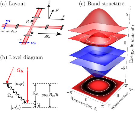
Figure 1: (a) Schematic layout: two nearly degenerate counter-propagating lasers differ in frequency by a very small $\delta\omega$, and are linearly polarized in the $\hat{x}$-$\hat{y}$ plane. An rf magnetic field $B_{\rm rf}\cos(\delta\omega t+\phi)$ is polarized along $\hat{z}$. A bias field $B_{0}\hat{x}$ brings the two Zeeman-resolved $m_{F}$ levels nearly into resonance. (b) Illustrative level diagram: the two $m_{F}$ states are coupled by optical and rf magnetic fields. The lattice potential formed by the retro-reflected lasers is omitted. (c) Band structure computed for $\Omega_{\rm R}=2t$, $\Omega_{\rm rf}=4t$, and $\phi=\pi/4$: the concentric-squircles of the Fermi-surface are obtained by filling the system to the third band, and are depicted by the white contours at the Fermi energy (also shown is the projection onto the $k_{+}$-$k_{-}$plane).

For particles with two spin states, our lattice model has four low-energy bands, and the third is shaped as a squarish, deformed, Mexican hat for a wide range of system parameters. By filling the system with fermions, we obtain a peculiar Fermi surface, consisting of the boundaries of a squarish ring, essentially two concentric squircles Guastia2005 . The particular shape of the Fermi surface suggests that nesting effects should be expected. To account for interactions, we develop an ${\rm SO}(3,1)\times{\rm SO}(3,1)$ description of the charge and spin degrees of freedom. Imperfect nesting along the diagonal connecting corners of the Fermi-surface gives rise to a coupled spin-charge-density wave (SCDW) instability at a critical interaction strength $U_{c}$. We calculate the imaginary part of the trace of the random phase approximation (RPA) susceptibility to study the collective excitations of the system. At the interaction strength $U_{c}$, a soft mode arises at the optimal nesting wave-vector ${\bf Q}$. The SCDW instability is in general incommensurate with the lattice, and is tunable by external parameters. In contrast with the usual behavior in 1D, our results show that in 2D a combined treatment of spin and charge degrees of freedom is essential to capture the possible instabilities of the system.

The physical system under study [Figs. 1(a)-(b)] consists of a sample of ultra cold atoms illuminated by two pairs of counter-propagating lasers with angular frequencies $\omega$ and $\omega+\delta\omega$ (where $\omega\gg\delta\omega$); a third pair of lasers, not shown, propagate along $\pm\hat{z}$ and create a 1D lattice, confining motion to the $\hat{x}-\hat{y}$ plane. Our model includes a static magnetic field $B_{0}$ along $\hat{x}$ and an rf magnetic field $B_{\rm rf}$ with angular frequency $\delta\omega$ along $\hat{z}$; rf coupling between atoms in spin dependent lattices has been studied both experimentally Lundblad2008 and theoretically Yi et al. (2008), where the resulting non-trivial real-space lattices suggested potential application to many body systems and quantum computation. In our case, the spin dependence results from the interplay of the laser and rf-magnetic fields.

As was observed in Refs. Deutsch and Jessen (1998); Dudarev et al. (2004); Sebby-Strabley et al. (2006), conventional spin independent (scalar) optical lattice potentials acquire additional spin-dependent terms near atomic resonance: the rank-1 and rank-2 tensor light shifts Deutsch and Jessen (1998). In the case of alkali atoms, adiabatic elimination of the angular momentum ${\mathcal{J}}=1/2$ (D1) and ${\mathcal{J}}=3/2$ (D2) excited states yields an effective Hamiltonian $H_{0}=U_{s}({\bf e}^{*}\cdot{\bf e})+iU_{v}{\vec{\mathcal{J}}}\cdot({\bf e}^{*}\times{\bf e})/\hbar$ for the ${\mathcal{J}}=1/2$ ground state atoms. $\bf e$ is the polarization vector of the optical electric field and the magnitude of the scalar and vector light shifts are related by $U_{v}=-2U_{s}\Delta_{\rm FS}/3(\omega-\omega_{0})$. Here, the fine-structure splitting is $\Delta_{\rm FS}=\omega_{3/2}-\omega_{1/2}$; $\hbar\omega_{1/2}$ and $\hbar\omega_{3/2}$ are the D1 and D2 transition energies; and $\omega_{0}=(2\omega_{1/2}+\omega_{3/2})/3$ is their suitable average. $U_{v}$ and $U_{s}$ can be independently specified with informed choices of laser frequency $\omega$ and intensity. We focus on a practical case, where the lasers are detuned far below atomic resonance $\omega_{0}-\omega\gg\Delta_{\rm FS}$, minimizing spontaneous emission and implying $|U_{s}|\gg|U_{v}|$ and $U_{s}<0$. We express momentum and energy in dimensions of $\hbar{{k_{r}}}=\hbar\omega/c$ and ${{E_{r}}}=\hbar^{2}{{k_{r}}}^{2}/2m$, the single-photon recoil momentum and energy, respectively, with $m$ the atomic mass.

The atomic Hamiltonian for the laser and magnetic fields in Figs. 1(a)-(b) is $H_{0}=U_{s}(\cos^{2}{{{k_{r}}}x}+\cos^{2}{{{k_{r}}}y})+g\mu_{B}{\vec{\mathcal{J}}}\cdot{\bf B}_{\rm eff}$ with ${\bf B}_{\rm eff}=B_{0}\hat{x}+B_{\rm rf}\cos(\delta\omega t+\phi)\hat{z}+\hat{z}(U_{v}/2g\mu_{B})\cos(\delta\omega t)\cos({{k_{r}}}x)\cos({{k_{r}}}y)$, where the vector light shift acts as an effective magnetic field and $B_{0}\gg B_{\rm rf},U_{v}/2g\mu_{B}$. Here, $\mu_{\rm B}$ is the Bohr magneton and $g$ is the Landé $g$-factor. We select $\hat{x}$ as the quantizing axes, transform into the frame rotating at $\delta\omega$, and make the rotating wave approximation to find

$${\bf B}_{\rm eff} =\left(B_{0}-\frac{\hbar\delta\omega}{g\mu_{B}}\right)\hat{x}-\frac{B_{\rm rf}}{2}\sin(\phi)\hat{y}+$$

$$\left[\frac{B_{\rm rf}}{2}\cos(\phi)+\frac{U_{v}}{4g\mu_{B}}\cos({{k_{r}}}x)\cos({{k_{r}}}y)\right]\hat{z}.$$

${\bf B}_{\rm eff}\cdot\hat{z}$ reaches its extrema on the sites of the optical lattice, giving a bias plus staggered Zeeman field. This proposal requires the simple retro-reflection of the existing “Raman” lasers discussed in Ref. Lin2009b , which were used to create an artificial magnetic field (there, $B_{\rm rf}$ was used only for state preparation). When $\left|U_{s}\right|\gg\left|U_{v}\right|,\left|g\mu_{B}B_{\rm rf}\right|$ the conventional tight-binding model Jaksch1998 , valid when $U_{s}\gtrsim 5{{E_{r}}}$, is slightly modified by the effective magnetic field evaluated on the lattice sites, yielding

$$H_{0} =-t\sum_{\left<{\bf i},{\bf j}\right>,s}c^{\dagger}_{{\bf i},s}c_{{\bf j},s}+\frac{\Omega_{\rm rf}}{2}\sum_{{\bf j}}\left(e^{i\phi}c^{\dagger}_{{\bf j},\uparrow}c_{{\bf j},\downarrow}+{\rm h.c.}\right)+$$

$$\frac{\Omega_{\rm R}}{2}\sum_{{\bf j}}\left(e^{i\pi(j_{x}+j_{y})}c^{\dagger}_{{\bf j},\uparrow}c_{{\bf j},\downarrow}+{\rm h.c.}\right).$$

$c_{{\bf j},s}$ is an annihilation operator (bosonic or fermionic) on site ${\bf j}$ with spin $s$; the hopping matrix element $t$ can be computed from the band structure of a sinusoidal lattice (for a $U_{s}=5{{E_{r}}}$ scalar lattice $t\approx 0.07{{E_{r}}}$); $\Omega_{\rm rf}=g\mu_{B}B_{\rm rf}$; and $\Omega_{\rm R}=U_{v}/2$. Since we focus on very small $\Omega_{R}\simeq t$, the detuning from atomic resonance can be quite large. For ⁴⁰K, with $\Delta_{FS}/2\pi=1.7{\ {\rm THz}}$, the detuning is $(\omega_{0}-\omega)/2\pi\approx 50\Delta_{FS}=86{\ {\rm THz}}$, yielding a laser wavelength $\approx 980{\ {\rm nm}}$, far detuned from the $770.1{\ {\rm nm}}$ (D1) and $766.7{\ {\rm nm}}$ (D2) transitions.

To determine the single-particle spectrum, we define spinor field operators $c_{\mathbf{j}}\equiv(c_{\mathbf{j},\uparrow},c_{\mathbf{j},\downarrow})^{T}$ and three component vectors $\mathbf{S}_{\mathbf{j}}=(S^{x}_{\mathbf{j}},S^{y}_{\mathbf{j}},S^{z}_{\mathbf{j}})^{T}=c_{\mathbf{j}}^{{\dagger}}\mathbf{\bf\check{\sigma}}c_{\mathbf{j}}/2$, where $\mathbf{\check{\sigma}}$ is the vector of Pauli matrices. Owing to the staggered Zeeman field, we introduce sublattices $A_{+}$ and $A_{-}$, where $A_{\pm}=\left\{(j_{x},j_{y})\big{|}(-1)^{j_{x}+j_{y}}=\pm 1\right\}$ and we define $a_{\mathbf{j},\pm}\equiv c_{\mathbf{j}}$ for $\mathbf{j}\in A_{\pm}$. In addition, we introduce vectors $\mathbf{B}_{\pm}=(\Omega_{\rm rf}\cos(\phi)\pm\Omega_{\rm R},-\Omega_{\rm rf}\sin(\phi),0)^{T}$ describing Zeeman fields on the $A_{\pm}$ sublattices. In this notation, the bare Hamiltonian is

$${H}_{0}=-t\sum_{\langle\mathbf{i},\mathbf{j}\rangle}(a^{{\dagger}}_{\mathbf{i,+}}a_{\mathbf{j,-}}+{\rm h.c.})+\sum_{\mathbf{j}\in A_{+}}\mathbf{S}^{T}_{\mathbf{j}}\cdot\mathbf{B}_{+}\sum_{\mathbf{j}\in A_{-}}\mathbf{S}^{T}_{\mathbf{j}}\cdot\mathbf{B}_{-}.$$

In terms of momentum field operators $\Psi^{{\dagger}}_{\mathbf{k}}=({a}^{{\dagger}}_{\mathbf{k},+,\uparrow},{a}^{{\dagger}}_{\mathbf{k},+,\downarrow},{a}^{{\dagger}}_{\mathbf{k},-,\uparrow},{a}^{{\dagger}}_{\mathbf{k},-,\downarrow})$, the Hamiltonian becomes ${H}_{0}=\sum_{\mathbf{k}}\Psi^{{\dagger}}_{\mathbf{k}}\mathbf{H}_{0\;\mathbf{k}}\Psi_{\mathbf{k}}$ where

$$\mathbf{H}_{0\;\mathbf{k}}=\left[\begin{array}[]{cc}\mathbf{\check{\sigma}}\cdot\mathbf{B}_{+}/2&-t\gamma_{\mathbf{k}}\mathbf{I}\\ -t\gamma_{\mathbf{k}}\mathbf{I}&\mathbf{\check{\sigma}}\cdot\mathbf{B}_{-}/2\end{array}\right].$$

Here, $\gamma_{\mathbf{k}}=4\cos(k_{+}/2)\cos(k_{-}/2)$, with $k_{\pm}=\pi(k_{x}\pm k_{y})/{{k_{r}}}$, $\mathbf{k}=(k_{+},k_{-})$ and $\bf I$ is the 2$\times$2 identity matrix. The summation goes over the entire Brillouin zone $-\pi<k_{+},k_{-}\leq\pi$, i.e., $\gamma_{\mathbf{k}}\geq 0$. The four eigenvalues of $\mathbf{H}_{0\;\mathbf{k}}$ are $\varepsilon_{\mathbf{k}}^{2}=(t\gamma_{\mathbf{k}})^{2}+(\Omega_{\rm rf}/2)^{2}+(\Omega_{\rm R}/2)^{2}\pm\Omega_{\rm rf}\sqrt{(t\gamma_{k})^{2}+(\Omega_{\rm R}\cos(\phi)/2)^{2}}$; together these eigenvalues constitute four bands [Fig. 1(c)]: the lowest band has a minimum at $\mathbf{k}=0$, whereas the third band can be shaped as a squarish, deformed Mexican hat. The second band may either exhibit the same trivial behavior as the first band, with a global minimum at $\mathbf{k}=0$ or have lines of degenerate minima along a square contour at the edge of the square Brillouin Zone. The fourth band always has lines of minima at the zone boundary.

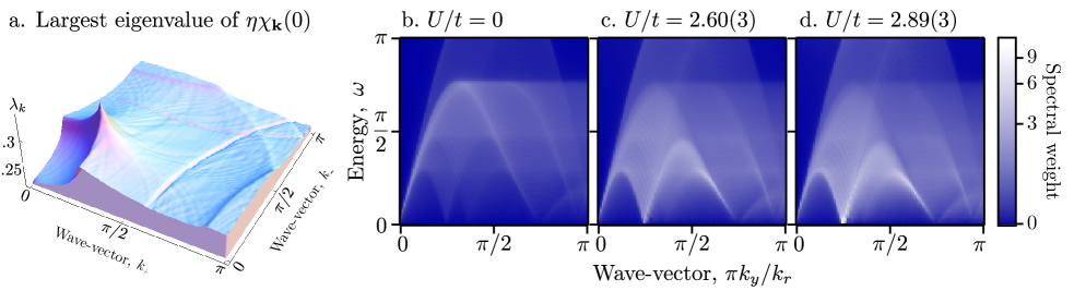
Figure 2: (a) Largest eigenvalue of the static susceptibility $\eta\chi_{\mathbf{k}}(0)$ as a function of $k_{+}$ and $k_{-}$. The peaks indicate the ${\bf Q}$ vectors for SCDW instabilities, and the largest peak marks the location of the most prominent nesting vector. Imaginary part of the trace of the susceptibility ${\rm Tr}[{\rm Im}\mathbf{\chi}_{\mathbf{k}}(\omega)]$ in logarithmic scale in the $k_{y}$-$\omega$ plane, with $k_{x}=0$, i.e., $k_{+}$=$-k_{-}$. (b) Without interactions a linearly dispersing sound mode is observed for small $k_{y}$. (c) For $U/t=2.60(3)$, spectral weight builds up for a second linear-dispersing mode, which starts from $\omega=0$ at $\pi k_{y}/{{k_{r}}}=\pi/4$. (d) For $U/t=2.89(3)$, the sharp increase of the intensity at $\omega=0$ with $\pi k_{y}/{{k_{r}}}=\pi/4$ signals the onset of SCDW instability.

Spin-charge-density-wave While the single-particle spectrum is valid for fermions and bosons, we now focus on spin-$1/2$ fermions with a Hamiltonian

$$H=H_{0}+H_{\rm int};\quad H_{\rm int}=U\sum_{\mathbf{j}}c^{{\dagger}}_{\mathbf{j},\uparrow}c^{{\dagger}}_{\mathbf{j},\downarrow}c_{\mathbf{j},\downarrow}c_{\mathbf{j},\uparrow}.$$ (1)

The interaction strength $U$ is proportional to the $s$-wave scattering length, and the Fermi energy is chosen to be in the third band. The resulting squarish Fermi surface is depicted by the white contours in Fig. 1(c) and is shaped like two concentric squircles. Nesting and local fermion-fermion interactions lead to spin- and charge- ordered phases in this system. We anticipate a second order phase transition when the coefficient of the second order term in the Landau free energy vanishes. Formally, we use the Hubbard-Stratonovich transformation to treat the interactions within a saddle point approximation (analogous to the time-dependent Hartree-Fock approximation).

Coexisting spin- and charge-density waves (SDW and CDW) have been studied in quasi-2D organics (a few coupled chains) using a Monte Carlo aproach Campbell . Conventional approaches to study SDW instabilities in the 2D Hubbard model neglect the contribution of charge density fluctuations Fradkin ; Negele , which are important here. In the following, we develop a generalized solution of 2D tight-binding models with local interactions and obtain a theory of SCDW instabilities.

In the coherent states formalism, the grand-canonical partition function is $Z=\int\mathrm{d}[c^{{\dagger}}]\mathrm{d}[c]e^{-{\cal S}[c^{{\dagger}},c]/\hbar}$, where ${\cal S}=\int_{0}^{\hbar\beta}\mathrm{d}\tau\left[\sum_{\mathbf{j}}c^{{\dagger}}_{\mathbf{j}}\left(\hbar\partial_{\tau}-\mu\right)c_{\mathbf{j}}+H_{0}+H_{\rm int}\right]$ is the Euclidean action and $\beta=1/k_{B}T$. We express the interaction term in a ${\rm SO}(3,1)$ invariant form $c^{{\dagger}}_{\mathbf{j},\uparrow}c^{{\dagger}}_{\mathbf{j},\downarrow}c_{\mathbf{j},\downarrow}c_{\mathbf{j},\uparrow}=(1/8)n_{\mathbf{j}}^{2}-(1/2){\mathbf{S}_{\mathbf{j}}}^{T}\cdot\mathbf{S}_{\mathbf{j}}$, with $n_{\mathbf{j}}=c_{\mathbf{j}}^{{\dagger}}c_{\mathbf{j}}$. The ${\rm SO}(3)$ invariance is required by rotational symmetry; the fact that the spin and charge terms have different signs reflects the Pauli principle, which requires a vanishing self-energy for a polarized state. The Hubbard-Stratonovich transformation renders the action quadratic in the fermion operators by introducing auxiliary bosonic fields, $\rho_{\pm}$ and $\mathbf{M}_{\pm}$, which couple to charge and spin density, respectively. For repulsive interactions the charge density term leads to a divergent integral. We resolve this problem by integrating along a contour parallel to the imaginary axis for $\rho_{\pm}$. Next, we introduce a source field $\mathbf{J}$ that couples to the charge and spin densities at each sublattice, and an eight-component vector $\mathbf{M}_{\mathbf{k},n}=(\rho_{\mathbf{k},+,n},\mathbf{M}_{\mathbf{k},+,n},\rho_{\mathbf{k},-,n},\mathbf{M}_{\mathbf{k},-,n})^{T}$ expressed in terms of momentum ${\bf k}$ and Matsubara frequency $\omega_{n}=\pi(2n+1)/\hbar\beta$. After integrating out the fermionic fields, we obtain a path-integral over the auxiliary bosonic field $\mathbf{M}_{\mathbf{k},n}$, which we evaluate in the saddle-point approximation. Notice that the saddle-point $\langle\mathbf{M}_{\mathbf{k},n}\rangle_{J}$ depends on the source field $\mathbf{J}$. We find that $\mathrm{d}\langle\mathbf{M}\rangle_{J}=\hbar U\mathbf{\chi}_{J}^{\rm RPA}\mathrm{d}\mathbf{J}$, where the generalized RPA susceptibility $(\mathbf{\chi}_{J}^{\rm RPA})^{-1}=\mathbf{\chi}_{J}^{-1}-\eta U$ is an $8\times 8$ matrix. The matrix $\eta={\rm Diag}(-1,1,1,1,-1,1,1,1)$ is a metric signature corresponding to the ${\rm SO}(3,1)\times{\rm SO}(3,1)$ group and $\mathbf{\chi}_{J}$ is the bare susceptibility for the renormalized Hamiltonian theory. By neglecting second order fluctuations of the Hubbard-Stratonovich fields, we obtain $\mathrm{d}\ln(Z[\mathbf{J}])=U^{-1}\langle\mathbf{M}\rangle^{{\dagger}}_{J}\cdot\mathrm{d}\mathbf{J}$. Neglecting now third- and higher-order terms in $\mathbf{J}$ we find $Z[\mathbf{J}]=Z[0]\exp(-{\cal S_{\rm eff}[\mathbf{J}]}/\hbar)$, where ${\cal S}_{\rm eff}=(-\hbar/U)\langle\mathbf{M}\rangle^{{\dagger}}_{0}\cdot\mathbf{J}-(\hbar^{2}/2)\mathbf{J}^{{\dagger}}\cdot(\mathbf{I}-U\mathbf{\chi}_{0}\eta)^{-1}\mathbf{\chi}_{0}\cdot\mathbf{J}$. The free energy may be determined by performing a Legendre transformation $\beta F[\langle\mathbf{M}\rangle_{J}]=U^{-1}\langle\mathbf{M}\rangle^{{\dagger}}_{J}\cdot\mathbf{J}-\ln(Z[\mathbf{J}])$ (see Ref. Negele ) which, up to quadratic order in the deviation $\Delta\langle\mathbf{M}\rangle_{J}\equiv\langle\mathbf{M}\rangle_{J}-\langle\mathbf{M}\rangle_{0}$ and without an additive constant reads

$$\beta F[\langle\mathbf{M}\rangle_{J}]=\frac{1}{2\hbar U^{2}}\left(\Delta\langle\mathbf{M}\rangle_{J}\right)^{{\dagger}}\cdot(\mathbf{\chi}_{0}^{\rm RPA})^{-1}\cdot\Delta\langle\mathbf{M}\rangle_{J}.$$ (2)

The susceptibility $\mathbf{\chi}_{0}^{\rm RPA}$ is evaluated in the absence of the source field, $\mathbf{J}=0$. For homogeneous phases, the susceptibility and the Hamiltonian become diagonal in momentum and frequency space. Thus, the Hamiltonian in the saddle-point approximation becomes

$$\mathbf{H}_{\mathbf{k}}=\mathbf{H}_{0\;\mathbf{k}}-\frac{U}{4N}\sum_{\mathbf{q},r,r^{\prime},\alpha}\mathbf{P}^{r}\eta^{r,r^{\prime}}{\rm Tr}[\mathbf{P}^{r^{\prime}}\mathbf{U}_{\mathbf{q}}\mathbf{I}^{(\alpha)}\mathbf{U}_{\mathbf{q}}^{{\dagger}}]n_{\rm F}(\tilde{\varepsilon}_{\mathbf{q}}^{(\alpha)}).$$ (3)

$\mathbf{P}^{r}=[{\rm Diag}(\mathbf{I},0)$, ${\rm Diag}(\sigma^{x},0)$, ${\rm Diag}(\sigma^{y},0)$, ${\rm Diag}(\sigma^{z},0)$, ${\rm Diag}(0,\mathbf{I})$, ${\rm Diag}(0,\sigma^{x})$, ${\rm Diag}(0,\sigma^{y})$, ${\rm Diag}(0,\sigma^{z})]^{T}$ are constant $4\times 4$ matrices; $N$ is the number of sites in a sublattice; $n_{\rm F}(z)=(e^{\beta z}+1)^{-1}$ is the Fermi distribution function; energy is measured with respect to the chemical potential $\tilde{\varepsilon}_{\mathbf{k}}^{(\alpha)}=\varepsilon_{\mathbf{k}}^{(\alpha)}-\mu$, and $\mathbf{U}_{\mathbf{q}}$ is a unitary matrix which diagonalizes

$$\mathbf{H}_{\mathbf{k}}=\sum_{\alpha}\mathbf{U}_{\mathbf{k}}\mathbf{I}^{(\alpha)}\mathbf{U}_{\mathbf{k}}^{{\dagger}}\varepsilon_{\mathbf{k}}^{(\alpha)},$$ (4)

with $\mathbf{I}^{(\alpha)}\equiv{\rm Diag}(\delta_{\alpha,1},\delta_{\alpha,2},\delta_{\alpha,3},\delta_{\alpha,4})$. Solving Eqs. (3) and (4) self consistently, we determine the RPA susceptibility $(\mathbf{\chi}_{0}^{\rm RPA})^{-1}=\mathbf{\chi}_{0}^{-1}-\eta U$, where the $k-$dependent susceptibility at zero source $\mathbf{\chi}_{0}$ is

$$\chi^{r,r^{\prime}}_{\mathbf{k}}(i\hbar\Omega_{n}) =\frac{1}{N}\sum_{\bf{p},\alpha,\beta}\frac{n_{F}(\tilde{\varepsilon}_{\mathbf{p}+\mathbf{k}}^{(\alpha)})-n_{F}(\tilde{\varepsilon}_{\mathbf{p}}^{(\beta)})}{\tilde{\varepsilon}_{\mathbf{p}+\mathbf{k}}^{(\alpha)}-\tilde{\varepsilon}_{\mathbf{p}}^{(\beta)}-i\hbar\Omega_{n}}T^{r,r^{\prime};\alpha,\beta}_{\mathbf{p}+\mathbf{k},\mathbf{p}},$$ (5)

$$T^{r,r^{\prime};\alpha,\beta}_{\mathbf{p}+\mathbf{k},\mathbf{p}} \equiv\frac{1}{2}{\rm Tr}[\mathbf{P}^{r}\mathbf{U}_{\mathbf{p}+\mathbf{k}}\mathbf{I}^{(\alpha)}\mathbf{U}_{\mathbf{p}+\mathbf{k}}^{{\dagger}}\mathbf{P}^{r^{\prime}}\mathbf{U}_{\mathbf{p}}\mathbf{I}^{(\beta)}\mathbf{U}_{\mathbf{p}}^{{\dagger}}].$$

Here $\Omega_{n}=2\pi n/\hbar\beta$ is the bosonic Matsubara frequency.

Static susceptibility The expression in Eq. (5) can be evaluated numerically with arbitrary precision. Though our approach is applicable for any temperature regime, we restrict ourselves to temperatures close to zero. First, we consider the static susceptibility $\chi_{\mathbf{k}}(0)$ and look for possible instabilities. The instability condition for repulsive interactions requires $U>U_{c}$, where $U_{c}$ is determined by $\det(\mathbf{\chi}^{-1}_{0}-U_{c}\eta)=0$. Since we avoid the van Hove singularity, the susceptibility is finite and the critical value $U_{c}$ is nonzero. It is related to the largest eigenvalue $\lambda_{\mathbf{Q}}$ of the matrix $\eta\chi_{\mathbf{k}}(0)$ by $U_{c}^{-1}=\max_{\mathbf{k}}\lambda_{\mathbf{k}}$. Thus, the instability condition becomes $\lambda_{\mathbf{Q}}U>1$, analogous to the Stoner criterium. Fig. 2(a) shows $\lambda_{\mathbf{Q}}$ for the Fermi surface in Fig. 1 ($\phi=\pi/4$, $\Omega_{\rm R}=2t$, $\Omega_{\rm rf}=4t$, $\mu=t$, and $k_{\rm B}T=10^{-3}t$). We calculated $\chi_{\mathbf{k}}(0)$ numerically on each point of a mesh with $240\times 240$ points. The peak with $\lambda_{\mathbf{Q}}=0.345(3)$, corresponding to the critical value of interactions $U_{c}/t=2.89(3)$, is located at $\mathbf{Q}=(\pi/4,\pi/4)$, where we expect an imperfect nesting between inner and outer lines of the Fermi surface [Fig. 1(c)], with $\varepsilon_{\mathbf{p}+\mathbf{Q}}^{(3)}\approx\varepsilon_{\mathbf{p}}^{(3)}$. For these system parameters, the eigenvector $V_{\mathbf{Q}}$ corresponding to this eigenvalue has an anti-ferrimagnetic character and is a mixture of both SDW and CDW, hence a SCDW. The details of the mixture are not universal.

The period of the SCDW $2\pi/|{\bf Q}|$ is in general incommensurate with the lattice period and is freely tunable by changing the vectors $\mathbf{B}_{\pm}$, and the chemical potential $\mu$. Nesting can also occur for other momenta, which results into smaller peaks forming the pattern shown in Fig. 2(a).

Had we neglected the coupling with charge and considered only the spin susceptibility, we would find at the same value of ${\bf Q}$ a much lower value for the critical interaction strength: $U_{c}/t=2.13(3)$ compared with $U_{c}/t=2.89(3)$ in the full calculation. In addition, when considering only charge excitations, no CDW instability occurs for repulsive interactions $U>0$. Thus, the coupling of charge and spin excitations, as developed here, is essential to the realization of a phenomenon which otherwise would only occur for attractive interactions $U<0$.

Collective excitations Equation (5) allows us to study the collective excitation spectra by analytically continuing $i\Omega_{n}\rightarrow\omega+i\kappa$ and looking at the imaginary part of the trace of the RPA susceptibility ${\rm Tr}[{\rm Im}\mathbf{\chi}^{\rm RPA}_{\mathbf{k}}(\omega)]$. For $\kappa=10^{-2}$ we find a linear dispersion spectrum in Fig. 2(b) in the long wavelength region (the Landau zero sound), which could have been anticipated, since we are considering a compressible zero-temperature Fermi liquid. At the interaction value $U_{c}/t=2.89(3)$ a soft linearly dispersing mode starting from $\mathbf{k}=\mathbf{Q}$ appears, signaling the onset of instability [Fig. 2(d)]. In ⁴⁰K, the collective excitation spectrum can be experimentally studied with an atomic analog of angle resolved photoemission spectroscopy Stewart2008 or by measuring the dynamic structure factor with energy and momentum sensitive Bragg spectroscopy Vogels2002 .

Conclusions We showed how to construct a system with a unique Fermi surface consisting of concentric squircles. The system has peculiar collective excitations, which we analyze in the RPA including both charge- and spin- density excitations. Our studies predict an anti-ferrimagnetic-like instability combining both CDW and SDW with a tunable incommensurate wave-vector, determined by the nesting properties of the Fermi surface, for sufficiently strong interactions. Moreover, we find that the usual approach – neglecting the coupling with density fluctuations – significantly underestimates the critical value of the interaction strength.

Acknowledgments We acknowledge the hospitality of the KITP Santa Barbara, supported by the National Science Foundation under Grant No. PHY05-51164, where this work was initiated. I.B.S. acknowledges the financial support of the ARO with funds from the DARPA OLE Program, and the NSF through the PFC at JQI. C.M.S. was partially supported by Netherlands Organization for Scientific Research NWO. We are indebted to D. Baeriswyl, G. Baym, A. Hemmerich, and A. Lazarides for fruitful discussions.

References

(1)I. Bloch, J. Dalibard, and W. Zwerger, Rev. Mod. Phys. 80, 885
(2008).
(2) M. Greiner et al., Nature 415, 39 (2002).
(3) O. Mandel et al., Nature 425, 937 (2003).
(4) P. J. Lee et al., Phys. Rev. Lett. 99, 020402 (2007).
(5) N. Lundblad et al., Phys. Rev. Lett. 100, 150401 (2008).
Dudarev et al. (2004)
A. M. Dudarev,
R. B. Diener,
I. Carusotto,
and Q. Niu,
Phys. Rev. Lett. 92,
153005 (2004).
(7)Revaz Ramazashvili, Phys. Rev. B 79, 184432 (2009).
(8)A. M. Essin,
J. E. Moore
and D. Vanderbilt,
Phys. Rev. Lett. 102,
146805 (2009).
(9)R. Li,
J. Wang
X.-L. Qi
and S.-C. Zhang,
Nat. Phys. 6,
284 (2010).
(10)M. Fernández Guasti,
A. Meléndez Cobarrubias
F. J. Renero Carrillo
and A. Cornejo Rodríguez,
Optik 116,
265 (2005).
Yi et al. (2008)
W. Yi,
A. J. Daley,
G. Pupillo, and
P. Zoller,
New Journal of Physics 10,
073015) (2008).
Sebby-Strabley
et al. (2006)
J. Sebby-Strabley,
M. Anderlini,
P. S. Jessen,
and J. V. Porto,
Phys. Rev. A 73,
033605 (2006).
Deutsch and Jessen (1998)
I. H. Deutsch and
P. S. Jessen,
Phys. Rev. A 57,
1972 (1998).
(14) Y.-J. Lin et al., Nature 462, 628 (2009).
(15) D. Jaksch et al., Phys. Rev. Lett. 81, 3108 (1998).
(16)S. Mazumdar et al., Phys. Rev. Lett. 82, 1522 (1999).
(17) E. Fradkin, Field Theories of Condensed Matter Systems (Addison-Wesley, Redwood City, CA, 1991).
(18) J. W. Negele and H. Orland, Quantum many-particle
systems (Westview, 1998).
(19)J. T. Stewart, J. P. Gaebler, and D. S. Jin, Nature 454, 744 (2008).
(20)J. M. Vogels et al., Phys. Rev. Lett. 88, 060402 (2002).