Dynamics of postcritically bounded polynomial semigroups II: fiberwise dynamics and the Julia sets

Abstract

We investigate the dynamics of semigroups generated by polynomial maps on the Riemann sphere such that the postcritical set in the complex plane is bounded. Moreover, we investigate the associated random dynamics of polynomials. Furthermore, we investigate the fiberwise dynamics of skew products related to polynomial semigroups with bounded planar postcritical set. Using uniform fiberwise quasiconformal surgery on a fiber bundle, we show that if the Julia set of such a semigroup is disconnected, then there exist families of uncountably many mutually disjoint quasicircles with uniform dilatation which are parameterized by the Cantor set, densely inside the Julia set of the semigroup. Moreover, we give a sufficient condition for a fiberwise Julia set $J_{\gamma}$ to satisfy that $J_{\gamma}$ is a Jordan curve but not a quasicircle, the unbounded component of $\hat{\mathbb{C}}\setminus J_{\gamma}$ is a John domain and the bounded component of $\mathbb{C}\setminus J_{\gamma}$ is not a John domain. We show that under certain conditions, a random Julia set is almost surely a Jordan curve, but not a quasicircle. Many new phenomena of polynomial semigroups and random dynamics of polynomials that do not occur in the usual dynamics of polynomials are found and systematically investigated.

1 Introduction

The theory of complex dynamical systems, which has its origin in the important work of Fatou and Julia in the 1910s, has been investigated by many people and discussed in depth. In particular, since D. Sullivan showed the famous “no wandering domain theorem” using Teichmüller theory in the 1980s, this subject has attracted many researchers from a wide area. For a general reference on complex dynamical systems, see Milnor’s textbook [14].

There are several areas in which we deal with generalized notions of classical iteration theory of rational functions. One of them is the theory of dynamics of rational semigroups (semigroups generated by holomorphic maps on the Riemann sphere $\hat{\mathbb{C}}$), and another one is the theory of random dynamics of holomorphic maps on the Riemann sphere.

In this paper, we will discuss these subjects. A rational semigroup is a semigroup generated by a family of non-constant rational maps on $\hat{\mathbb{C}}$, where $\hat{\mathbb{C}}$ denotes the Riemann sphere, with the semigroup operation being functional composition ([11]). A polynomial semigroup is a semigroup generated by a family of non-constant polynomial maps. Research on the dynamics of rational semigroups was initiated by A. Hinkkanen and G. J. Martin ([11]), who were interested in the role of the dynamics of polynomial semigroups while studying various one-complex-dimensional moduli spaces for discrete groups, and by F. Ren and Z. Gong ([10]) and others, who studied such semigroups from the perspective of random dynamical systems. Moreover, the research on rational semigroups is related to that on “iterated function systems” in fractal geometry. In fact, the Julia set of a rational semigroup generated by a compact family has “ backward self-similarity” (cf. [22, 23]). [17] is a very nice (and short) article for an introduction to the dynamics of rational semigroups. For other research on rational semigroups, see [37, 18, 19, 35, 36], and [21]–[33].

Research on the dynamics of rational semigroups is also directly related to that on the random dynamics of holomorphic maps. The first study in this direction was by Fornaess and Sibony ([8]), and much research has followed. (See [2, 4, 5, 3, 9, 27, 30, 31, 32, 33, 34].)

We remark that complex dynamical systems can be used to describe some mathematical models. For example, the behavior of the population of a certain species can be described as the dynamical system of a polynomial $f(z)=az(1-z)$ such that $f$ preserves the unit interval and the postcritical set in the plane is bounded (cf. [7]). From this point of view, it is very important to consider the random dynamics of such polynomials (see also Example 1.4). The results of this paper might have applications to mathematical models. For the random dynamics of polynomials on the unit interval, see [20].

We shall give some definitions for the dynamics of rational semigroups:

Definition 1.1 ([11, 10]).

Let $G$ be a rational semigroup. We set

$$F(G)=\{z\in\hat{\mathbb{C}}\mid G\mbox{ is normal in a neighborhood of $z$}\},\ J(G)=\hat{\mathbb{C}}\setminus F(G).$$

$F(G)$ is called the Fatou set of $G$ and $J(G)$ is called the Julia set of $G$. We let $\langle h_{1},h_{2},\ldots\rangle$ denote the rational semigroup generated by the family $\{h_{i}\}.$ The Julia set of the semigroup generated by a single map $g$ is denoted by $J(g).$

Definition 1.2.

For each rational map $g:\hat{\mathbb{C}}\rightarrow\hat{\mathbb{C}}$, we set $CV(g):=\{\mbox{all critical values of }g:\hat{\mathbb{C}}\rightarrow\hat{\mathbb{C}}\}.$ Moreover, for each polynomial map $g:\hat{\mathbb{C}}\rightarrow\hat{\mathbb{C}}$, we set $CV^{\ast}(g):=CV(g)\setminus\{\infty\}.$ For a rational semigroup $G$, we set

$$P(G):=\overline{\bigcup_{g\in G}CV(g)}\ (\subset\hat{\mathbb{C}}).$$

This is called the postcritical set of $G.$ Furthermore, for a polynomial semigroup $G$, we set $P^{\ast}(G):=P(G)\setminus\{\infty\}.$ This is called the planar postcritical set (or finite postcritical set) of $G.$ We say that a polynomial semigroup $G$ is postcritically bounded if $P^{\ast}(G)$ is bounded in $\mathbb{C}.$

Remark 1.3.

Let $G$ be a rational semigroup generated by a family $\Lambda$ of rational maps. Then, we have that $P(G)=\overline{\cup_{g\in G\cup\{Id\}}\ g(\cup_{h\in\Lambda}CV(h))}$, where Id denotes the identity map on $\hat{\mathbb{C}}$, and that $g(P(G))\subset P(G)$ for each $g\in G.$ Using this formula, one can understand how the set $P(G)$ (resp. $P^{\ast}(G)$) spreads in $\hat{\mathbb{C}}$ (resp. $\mathbb{C}$). In fact, in Section 3.4, using the above formula, we present a way to construct examples of postcritically bounded polynomial semigroups (with some additional properties). Moreover, from the above formula, one may, in the finitely generated case, use a computer to see if a polynomial semigroup $G$ is postcritically bounded much in the same way as one verifies the boundedness of the critical orbit for the maps $f_{c}(z)=z^{2}+c.$

Example 1.4.

Let $\Lambda:=\{h(z)=cz^{a}(1-z)^{b}\mid a,b\in\mathbb{N},\ c>0,\ c(\frac{a}{a+b})^{a}(\frac{b}{a+b})^{b}$ $\leq 1\}$ and let $G$ be the polynomial semigroup generated by $\Lambda.$ Since for each $h\in\Lambda$, $h([0,1])\subset[0,1]$ and $CV^{\ast}(h)\subset[0,1]$, it follows that each subsemigroup $H$ of $G$ is postcritically bounded.

Remark 1.5.

It is well-known that for a polynomial $g$ with $\deg(g)\geq 2$, $P^{\ast}(\langle g\rangle)$ is bounded in $\mathbb{C}$ if and only if $J(g)$ is connected ([14, Theorem 9.5]).

As mentioned in Remark 1.5, the planar postcritical set is one piece of important information regarding the dynamics of polynomials.

When investigating the dynamics of polynomial semigroups, it is natural for us to discuss the relationship between the planar postcritical set and the Julia set. The first question in this regard is: “Let $G$ be a polynomial semigroup such that each element $g\in G$ is of degree at least two. Is $J(G)$ necessarily connected when $P^{\ast}(G)$ is bounded in $\mathbb{C}$?” The answer is NO. In fact, in [37, 29, 30, 19, 31, 32], we find many examples of postcritically bounded polynomial semigroups $G$ with disconnected Julia set such that for each $g\in G$, $\deg(g)\geq 2.$ Thus, it is natural to ask the following questions.

Problem 1.6.

(1) What properties does $J(G)$ have if $P^{\ast}(G)$ is bounded in $\mathbb{C}$ and $J(G)$ is disconnected? (2) Can we classify postcritically bounded polynomial semigroups?

Applying the results in [29, 30], we investigate the dynamics of every sequence, or fiberwise dynamics of the skew product associated with the generator system (cf. Section 3.1). Moreover, we investigate the random dynamics of polynomials acting on the Riemann sphere. Let us consider a polynomial semigroup $G$ generated by a compact family $\Gamma$ of polynomials. For each sequence $\gamma=(\gamma_{1},\gamma_{2},\gamma_{3},\ldots)\in\Gamma^{\mathbb{N}}$, we examine the dynamics along the sequence $\gamma$, that is, the dynamics of the family of maps $\{\gamma_{n}\circ\cdots\circ\gamma_{1}\}_{n=1}^{\infty}$. We note that this corresponds to the fiberwise dynamics of the skew product (see Section 3.1) associated with the generator system $\Gamma.$ We show that if $G$ is postcritically bounded, $J(G)$ is disconnected, and $G$ is generated by a compact family $\Gamma$ of polynomials, then, for almost every sequence $\gamma\in\Gamma^{\mathbb{N}}$, there exists exactly one bounded component $U_{\gamma}$ of the Fatou set of $\gamma$, the Julia set of $\gamma$ has Lebesgue measure zero, there exists no non-constant limit function in $U_{\gamma}$ for the sequence $\gamma$, and for any point $z\in U_{\gamma}$ the orbit of $z$ along $\gamma$ tends to the interior of the smallest filled-in Julia set $\hat{K}(G)$ (see Definition 2.7) of $G$ (cf. Theorem 3.11, Corollary 3.21). Moreover, using uniform fiberwise quasiconformal surgery ([30]), we find sub-skew products $\overline{f}$ such that $\overline{f}$ is hyperbolic (see Definition 3.10) and such that every fiberwise Julia set of $\overline{f}$ is a $K$-quasicircle, where $K$ is a constant not depending on the fibers (cf. Theorem 3.11, statement 3). Reusing the uniform fiberwise quasiconformal surgery, we show that if $G$ is a postcritically bounded polynomial semigroup with disconnected Julia set, then for any non-empty open subset $V$ of $J(G)$, there exists a $2$-generator subsemigroup $H$ of $G$ such that $J(H)$ is the disjoint union of a “Cantor family of quasicircles” (a family of quasicircles parameterized by a Cantor set) with uniform distortion, and such that $J(H)\cap V\neq\emptyset$ (cf. Theorem 3.14). Note that the uniform fiberwise quasiconformal surgery is based on solving uncountably many Beltrami equations.

We also investigate (semi-)hyperbolic (see Definition 3.12), postcritically bounded, polynomial semigroups generated by a compact family $\Gamma$ of polynomials. Let $G$ be such a semigroup with disconnected Julia set, and suppose that there exists an element $g\in G$ such that $J(g)$ is not a Jordan curve. Then, we give a (concrete) sufficient condition for a sequence $\gamma\in\Gamma^{\mathbb{N}}$ to give rise to the following situation ($\ast$): the Julia set of $\gamma$ is a Jordan curve but not a quasicircle, the basin of infinity $A_{\gamma}$ is a John domain, and the bounded component $U_{\gamma}$ of the Fatou set is not a John domain (cf. Theorem 3.18, Corollary 3.22). From this result, we show that for almost every sequence $\gamma\in\Gamma^{\mathbb{N}}$, situation $(\ast)$ holds. In fact, in this paper, under the above assumption, we find a set ${\cal A}$ of $\gamma$ with $(\ast)$ which is much larger than a set ${\cal U}$ of $\gamma$ with $(\ast)$ given in [30]. Moreover, we classify hyperbolic two-generator postcritically bounded polynomial semigroups $G$ with disconnected Julia set and we also completely classify the fiberwise Julia sets $J_{\gamma}$ in terms of the information of $\gamma$ (Theorem 3.19). Note that situation $(\ast)$ cannot hold in the usual iteration dynamics of a single polynomial map $g$ with $\deg(g)\geq 2$ (Remark 3.23).

The key to investigating the dynamics of postcritically bounded polynomial semigroups is the density of repelling fixed points in the Julia set ([11, 10]), which can be shown by an application of the Ahlfors five island theorem, and the lower semi-continuity of $\gamma\mapsto J_{\gamma}$ ([12]), which is a consequence of potential theory. Moreover, one of the keys to investigating the fiberwise dynamics of skew products is, the observation of non-constant limit functions (cf. Lemma 5.4 and [23]). The key to investigating the dynamics of semi-hyperbolic polynomial semigroups is, the continuity of the map $\gamma\mapsto J_{\gamma}$ (this is highly nontrivial; see [23]) and the Johnness of the basin $A_{\gamma}$ of infinity (cf. [25]). Note that the continuity of the map $\gamma\mapsto J_{\gamma}$ does not hold in general, if we do not assume semi-hyperbolicity. Moreover, one of the original aspects of this paper is the idea of “combining both the theory of rational semigroups and that of random complex dynamics”. It is quite natural to investigate both fields simultaneously. However, no study (except the works of the author of this paper) thus far has done so.

Furthermore, in Section 3.4 and [29, 30], we provide a way of constructing examples of postcritically bounded polynomial semigroups with some additional properties (disconnectedness of the Julia set, semi-hyperbolicity, hyperbolicity, etc.) (cf. Proposition 3.24, [29, 30]). For example, by Proposition 3.24, there exists a $2$-generator postcritically bounded polynomial semigroup $G=\langle h_{1},h_{2}\rangle$ with disconnected Julia set such that $h_{1}$ has a Siegel disk.

As we see in Example 1.4, Section 3.4, and [29, 30], it is not difficult to construct many examples for which we can verify the hypothesis “postcritically bounded”, so the class of postcritically bounded polynomial semigroups is very wide.

Throughout the paper, we will see many new phenomena in polynomial semigroups or random dynamics of polynomials that do not occur in the usual dynamics of polynomials. Moreover, these new phenomena are systematically investigated.

In Section 3, we present the main results of this paper. We give some tools in Section 4. The proofs of the main results are given in Section 5.

There are many applications of the results of postcritically bounded polynomial semigroups in many directions. In the sequel [31, 27, 33, 34], we investigate the Markov process on $\hat{\mathbb{C}}$ associated with the random dynamics of polynomials and we consider the probability $T_{\infty}(z)$ of tending to $\infty\in\hat{\mathbb{C}}$ starting with the initial value $z\in\hat{\mathbb{C}}.$ Applying many results of [29], it will be shown in [34] that if the associated polynomial semigroup $G$ is postcritically bounded and the Julia set is disconnected, then the chaos of the averaged system disappears due to the cooperation of generators (cooperation principle), and the function $T_{\infty}$ defined on $\hat{\mathbb{C}}$ has many interesting properties which are similar to those of the devil’s staircase (the Cantor function). Such “singular functions on the complex plane” appear very naturally in random dynamics of polynomials and the results of this paper (for example, the results on the space of all connected components of a Julia set) are the keys to investigating them. (The above results have been announced in [31, 27, 26, 32].)

In [29], we find many fundamental and useful results on the connected components of Julia sets of postcritically bounded polynomial semigroups. In [30], we classify (semi-)hyperbolic, postcritically bounded, compactly generated polynomial semigroups. In the sequel [19], we give some further results on postcritically bounded polynomial semigroups, by using many results in [29, 30], and this paper. Moreover, in the sequel [28], we define a new kind of cohomology theory, in order to investigate the action of finitely generated semigroups (iterated function systems), and we apply it to the study of the dynamics of postcritically bounded polynomial semigroups.

2 Preliminaries

In this section we give some basic notations and definitions, and we present some results in [29, 30], which we need to state the main results of this paper.

Definition 2.1.

We set Rat : $=\{h:\hat{\mathbb{C}}\rightarrow\hat{\mathbb{C}}\mid h\mbox{ is a non-constant rational map}\}$ endowed with distance $\eta$ defined as $\eta(f,g):=\sup_{z\in\hat{\mathbb{C}}}d(f(z),g(z))$, where $d$ denotes the spherical distance on $\hat{\mathbb{C}}.$ We set Poly :$=\{h:\hat{\mathbb{C}}\rightarrow\hat{\mathbb{C}}\mid h\mbox{ is a non-constant polynomial}\}$ endowed with the relative topology from Rat. Moreover, we set Poly${}_{\deg\geq 2}:=\{g\in\mbox{Poly}\mid\deg(g)\geq 2\}$ endowed with the relative topology from Rat.

Remark 2.2.

Let $d\geq 1$, $\{p_{n}\}_{n\in\mathbb{N}}$ be a sequence of polynomials of degree $d$, and $p$ be a polynomial. Then $p_{n}\rightarrow p$ in Poly if and only if $p$ is of degree $d$ and the coefficients of $p_{n}$ converge appropriately.

Definition 2.3.

Let ${\cal G}$ be the set of all postcritically bounded polynomial semigroups $G$ such that each element of $G$ is of degree at least two. Furthermore, we set ${\cal G}_{con}=\{G\in{\cal G}\mid J(G)\mbox{ is connected}\}$ and ${\cal G}_{dis}=\{G\in{\cal G}\mid J(G)\mbox{ is disconnected}\}.$

Definition 2.4.

For a polynomial semigroup $G$, we denote by ${\cal J}={\cal J}_{G}$ the set of all connected components $J$ of $J(G)$ such that $J\subset\mathbb{C}.$ Moreover, we denote by $\hat{{\cal J}}=\hat{{\cal J}}_{G}$ the set of all connected components of $J(G).$

Remark 2.5.

If a polynomial semigroup $G$ is generated by a compact set in Poly_deg≥2, then $\infty\in F(G)$ and thus ${\cal J}=\hat{{\cal J}}.$

Definition 2.6 ([29]).

For any connected sets $K_{1}$ and $K_{2}$ in $\mathbb{C},\$ “$K_{1}\leq K_{2}$” indicates that $K_{1}=K_{2}$, or $K_{1}$ is included in a bounded component of $\mathbb{C}\setminus K_{2}.$ Furthermore, “$K_{1}<K_{2}$” indicates $K_{1}\leq K_{2}$ and $K_{1}\neq K_{2}.$ Note that “$\leq$” is a partial order in the space of all non-empty compact connected sets in $\mathbb{C}.$ This “$\leq$” is called the surrounding order.

Definition 2.7 ([29]).

For a polynomial semigroup $G$, we set

$$\hat{K}(G):=\{z\in\mathbb{C}\mid\bigcup_{g\in G}\{g(z)\}\mbox{ is bounded in }\mathbb{C}\}$$

and call $\hat{K}(G)$ the smallest filled-in Julia set of $G.$ For a polynomial $g$, we set $K(g):=\hat{K}(\langle g\rangle).$ For a set $A\subset\hat{\mathbb{C}}$, we denote by int$(A)$ the set of all interior points of $A.$ For a polynomial semigroup $G$ with $\infty\in F(G)$, we denote by $F_{\infty}(G)$ the connected component of $F(G)$ containing $\infty.$ Moreover, for a polynomial $g$ with $\deg(g)\geq 2$, we set $F_{\infty}(g):=F_{\infty}(\langle g\rangle).$

The following three results in [29] are needed to state the main result in this paper.

Theorem 2.8 ([29]).

Let $G\in{\cal G}$ (possibly generated by a non-compact family). Then we have all of the following.

1. We have $({\cal J},\ \leq)$ is totally ordered.

2. Each connected component of $F(G)$ is either simply or doubly connected.

3. For any $g\in G$ and any connected component $J$ of $J(G)$, we have that $g^{-1}(J)$ is connected. Let $g^{\ast}(J)$ be the connected component of $J(G)$ containing $g^{-1}(J).$ If $J\in{\cal J}$, then $g^{\ast}(J)\in{\cal J}.$ If $J_{1},J_{2}\in{\cal J}$ and $J_{1}\leq J_{2},\$ then $g^{-1}(J_{1})\leq g^{-1}(J_{2})$ and $g^{\ast}(J_{1})\leq g^{\ast}(J_{2}).$

Theorem 2.9 ([29]).

Let $G\in{\cal G}_{dis}$ (possibly generated by a non-compact family). Then we have all of the following.

1. We have $\infty\in F(G)$. Thus ${\cal J}=\hat{{\cal J}}.$

2. The component $F_{\infty}(G)$ of $F(G)$ containing $\infty$ is simply connected. Furthermore, the element $J_{\max}=J_{\max}(G)\in{\cal J}$ containing $\partial F_{\infty}(G)$ is the unique element of ${\cal J}$ satisfying that $J\leq J_{\max}$ for each $J\in{\cal J}.$

3. There exists a unique element $J_{\min}=J_{\min}(G)\in{\cal J}$ such that $J_{\min}\leq J$ for each element $J\in{\cal J}.$

4. We have that $\mbox{{\em int}}(\hat{K}(G))\neq\emptyset.$

For the figures of the Julia sets of semigroups $G\in{\cal G}_{dis}$, see Figure 1.

Proposition 2.10 ([29]).

Let $G$ be a polynomial semigroup generated by a compact subset $\Gamma$ of Poly${}_{\deg\geq 2}.$ Suppose that $G\in{\cal G}_{dis}.$ Then, there exists an element $h_{1}\in\Gamma$ with $J(h_{1})\subset J_{\max}$ and there exists an element $h_{2}\in\Gamma$ with $J(h_{2})\subset J_{\min}.$

3 Main results

In this section, we present the main results of this paper. The proofs of the results are given in Section 5.

3.1 Fiberwise dynamics and Julia sets

We present some results on the fiberwise dynamics of the skew product related to a postcritically bounded polynomial semigroup with disconnected Julia set. In particular, using the uniform fiberwise quasiconformal surgery on a fiber bundle, we show the existence of families of quasicircles with uniform distortion parameterized by the Cantor set densely inside the Julia set of such a semigroup. The proofs are given in Section 5.1.

Definition 3.1 ([23, 25]).

1. Let $X$ be a compact metric space, $g:X\rightarrow X$ a continuous map, and $f:X\times\hat{\mathbb{C}}\rightarrow X\times\hat{\mathbb{C}}$ a continuous map. We say that $f$ is a rational skew product (or fibered rational map on the trivial bundle $X\times\hat{\mathbb{C}}$) over $g:X\rightarrow X$, if $\pi\circ f=g\circ\pi$ where $\pi:X\times\hat{\mathbb{C}}\rightarrow X$ denotes the canonical projection, and if, for each $x\in X$, the restriction $f_{x}:=f|_{\pi^{-1}(\{x\})}:\pi^{-1}(\{x\})\rightarrow\pi^{-1}(\{g(x)\})$ of $f$ is a non-constant rational map, under the canonical identification $\pi^{-1}(\{x^{\prime}\})\cong\hat{\mathbb{C}}$ for each $x^{\prime}\in X.$ Let $d(x)=\deg(f_{x})$, for each $x\in X.$ Let $f_{x,n}$ be the rational map defined by: $f_{x,n}(y)=\pi_{\hat{\mathbb{C}}}(f^{n}(x,y))$, for each $n\in\mathbb{N},x\in X$ and $y\in\hat{\mathbb{C}}$, where $\pi_{\hat{\mathbb{C}}}:X\times\hat{\mathbb{C}}\rightarrow\hat{\mathbb{C}}$ is the projection map.

   Moreover, if $f_{x,1}$ is a polynomial for each $x\in X$, then we say that $f:X\times\hat{\mathbb{C}}\rightarrow X\times\hat{\mathbb{C}}$ is a polynomial skew product over $g:X\rightarrow X.$

2. Let $\Gamma$ be a compact subset of Rat. We set $\Gamma^{\mathbb{N}}:=\{\gamma=(\gamma_{1},\gamma_{2},\ldots)\mid\forall j,\gamma_{j}\in\Gamma\}$ endowed with the product topology. This is a compact metric space. Let $\sigma:\Gamma^{\mathbb{N}}\rightarrow\Gamma^{\mathbb{N}}$ be the shift map, which is defined by $\sigma(\gamma_{1},\gamma_{2},\ldots):=(\gamma_{2},\gamma_{3},\ldots).$ Moreover, we define a map $f:\Gamma^{\mathbb{N}}\times\hat{\mathbb{C}}\rightarrow\Gamma^{\mathbb{N}}\times\hat{\mathbb{C}}$ by: $(\gamma,y)\mapsto(\sigma(\gamma),\gamma_{1}(y)),\$ where $\gamma=(\gamma_{1},\gamma_{2},\ldots).$ This is called the skew product associated with the family $\Gamma$ of rational maps. Note that $f_{\gamma,n}(y)=\gamma_{n}\circ\cdots\circ\gamma_{1}(y).$

Remark 3.2.

Regarding item 1 of Definition 3.1, the map $f^{n}|_{\pi^{-1}(\{x\})}:\pi^{-1}(\{x\})\rightarrow\pi^{-1}(\{g^{n}(x)\})$ is equal to the rational map $f_{g^{n-1}(x)}\circ\cdots\circ f_{x}$ under the canonical identification $\pi^{-1}(\{x^{\prime}\})\cong\hat{\mathbb{C}}$ for each $x^{\prime}\in X.$ Thus, if we consider the dynamics of $f$, then we can investigate the dynamics of all sequences generated by the family $\{f_{x}\}_{x\in X}$ and the map $g.$

Remark 3.3.

Let $f:X\times\hat{\mathbb{C}}\rightarrow X\times\hat{\mathbb{C}}$ be a rational skew product over $g:X\rightarrow X.$ Then the function $x\mapsto d(x)$ is continuous in $X.$ For, since $f$ is continuous, the map $x\mapsto f_{x}\in\mbox{Rat}$ is continuous. Moreover, the function $g\in\mbox{Rat}\mapsto\deg(g)\in\mathbb{R}$ is continuous ([1, Theorem 2.8.2]). Thus, $x\mapsto d(x)$ is continuous.

Definition 3.4 ([23, 25]).

Let $f:X\times\hat{\mathbb{C}}\rightarrow X\times\hat{\mathbb{C}}$ be a rational skew product over $g:X\rightarrow X.$ Then, for each $x\in X$ and $n\in\mathbb{N}$, we set $f_{x}^{n}:=f^{n}|_{\pi^{-1}(\{x\})}:\pi^{-1}(\{x\})\rightarrow\pi^{-1}(\{g^{n}(x)\})\subset X\times\hat{\mathbb{C}}.$ For each $x\in X$, we denote by $F_{x}(f)$ the set of points $y\in\hat{\mathbb{C}}$ which has a neighborhood $U$ in $\hat{\mathbb{C}}$ such that $\{f_{x,n}:U\rightarrow\hat{\mathbb{C}}\}_{n\in\mathbb{N}}$ is normal. Moreover, we set $F^{x}(f):=\{x\}\times F_{x}(f)\ (\subset X\times\hat{\mathbb{C}}).$ We set $J_{x}(f):=\hat{\mathbb{C}}\setminus F_{x}(f).$ Moreover, we set $J^{x}(f):=\{x\}\times J_{x}(f)$ $(\subset X\times\hat{\mathbb{C}}).$ These sets $J^{x}(f)$ and $J_{x}(f)$ are called the fiberwise Julia sets. Moreover, we set $\tilde{J}(f):=\overline{\bigcup_{x\in X}J^{x}(f)}$, where the closure is taken in the product space $X\times\hat{\mathbb{C}}.$ For each $x\in X$, we set $\hat{J}^{x}(f):=\pi^{-1}(\{x\})\cap\tilde{J}(f).$ Moreover, we set $\hat{J}_{x}(f):=\pi_{\hat{\mathbb{C}}}(\hat{J}^{x}(f)).$ We set $\tilde{F}(f):=(X\times\hat{\mathbb{C}})\setminus\tilde{J}(f).$

Remark 3.5 ([23, 25]).

• We have $f_{x}^{-1}(J_{g(x)})=J_{x}$, $f_{x}(J_{x})=J_{g(x)}$, $f(\tilde{J}(f))\subset\tilde{J}(f)$, $\hat{J}^{x}(f)\supset J^{x}(f)$ and $\hat{J}_{x}(f)\supset J_{x}(f).$ However, for the last one, strict containment can occur. For example, let $h_{1}$ be a polynomial having a Siegel disk with center $z_{1}\in\mathbb{C}.$ Let $h_{2}$ be a polynomial such that $z_{1}$ is a repelling fixed point of $h_{2}.$ Let $\Gamma=\{h_{1},h_{2}\}.$ Let $f:\Gamma\times\hat{\mathbb{C}}\rightarrow\Gamma\times\hat{\mathbb{C}}$ be the skew product associated with the family $\Gamma.$ Let $x=(h_{1},h_{1},h_{1},\ldots)\in\Gamma^{\mathbb{N}}.$ Then, $(x,z_{1})\in\hat{J}^{x}(f)\setminus J^{x}(f)$ and $z_{1}\in\hat{J}_{x}(f)\setminus J_{x}(f).$

  If $g$ is an open and surjective map (e.g. the shift map $\sigma:\Gamma^{\mathbb{N}}\rightarrow\Gamma^{\mathbb{N}}$), then $f^{-1}(\tilde{J}(f))=f(\tilde{J}(f))=\tilde{J}(f)$ ([23, Lemma 2.4]). For more details, see [23, 25].

• Let $\Gamma$ be a compact subset of Rat and let $f:\Gamma^{\mathbb{N}}\times\hat{\mathbb{C}}\rightarrow\Gamma^{\mathbb{N}}\times\hat{\mathbb{C}}$ be the skew product associated with $\Gamma.$ Let $G$ be the rational semigroup generated by $\Gamma$ (thus $G=\{g_{i_{1}}\circ\cdots\circ g_{i_{n}}\mid n\in\mathbb{N},\forall g_{i_{j}}\in\Gamma\}$). If $\sharp(J(G))\geq 3$, then $\pi_{\hat{\mathbb{C}}}(\tilde{J}(f))=J(G)$ ([30, Lemma 3.5]). From this result, we can apply the results of the dynamics of $f$ to the dynamics of $G.$

Definition 3.6 ([30]).

Let $f:X\times\hat{\mathbb{C}}\rightarrow X\times\hat{\mathbb{C}}$ be a polynomial skew product over $g:X\rightarrow X.$ Then for each $x\in X$, we set $K_{x}(f):=\{y\in\hat{\mathbb{C}}\mid\{f_{x,n}(y)\}_{n\in\mathbb{N}}\mbox{ is bounded }$ in $\mathbb{C}\}$, and $A_{x}(f):=\{y\in\hat{\mathbb{C}}\mid f_{x,n}(y)\rightarrow\infty,\ n\rightarrow\infty\}.$ Moreover, we set $K^{x}(f):=\{x\}\times K_{x}(f)\ (\subset X\times\hat{\mathbb{C}})$ and $A^{x}(f):=\{x\}\times A_{x}(f)\ (\subset X\times\hat{\mathbb{C}}).$

Definition 3.7 ([29]).

Let $G$ be a polynomial semigroup generated by a subset $\Gamma$ of Poly${}_{\deg\geq 2}.$ Suppose $G\in{\cal G}_{dis}.$ Then we set $\Gamma_{\min}:=\{h\in\Gamma\mid J(h)\subset J_{\min}\},$ where $J_{\min}$ denotes the unique minimal element in $({\cal J},\ \leq)$ in statement 3 of Theorem 2.9. Furthermore, if $\Gamma_{\min}\neq\emptyset$, let $G_{\min,\Gamma}$ be the subsemigroup of $G$ that is generated by $\Gamma_{\min}.$

Remark 3.8.

Let $G$ be a polynomial semigroup generated by a compact subset $\Gamma$ of Poly${}_{\deg\geq 2}.$ Suppose $G\in{\cal G}_{dis}.$ Then, by Proposition 2.10, we have $\Gamma_{\min}\neq\emptyset$ and $\Gamma\setminus\Gamma_{\min}\neq\emptyset.$ Moreover, $\Gamma_{\min}$ is a compact subset of $\Gamma.$ For, if $\{h_{n}\}_{n\in\mathbb{N}}\subset\Gamma_{\min}$ and $h_{n}\rightarrow h_{\infty}$ in $\Gamma$, then for each repelling periodic point $z_{0}\in J(h_{\infty})$ of $h_{\infty}$, we have that $d(z_{0},J(h_{n}))\rightarrow 0$ as $n\rightarrow\infty$, which implies that $z_{0}\in J_{\min}$ and thus $h_{\infty}\in\Gamma_{\min}.$

Notation: Let ${\cal F}:=\{\varphi_{n}\}_{n\in\mathbb{N}}$ be a sequence of meromorphic functions in a domain $V.$ We say that a meromorphic function $\psi$ is a limit function of ${\cal F}$ if there exists a strictly increasing sequence $\{n_{j}\}_{j\in\mathbb{N}}$ of positive integers such that $\varphi_{n_{j}}\rightarrow\psi$ locally uniformly on $V$, as $j\rightarrow\infty.$

Definition 3.9.

Let $\Gamma$ and $S$ be non-empty subsets of Poly_deg≥2 with $S\subset\Gamma.$ We set

$$R(\Gamma,S):=\left\{\gamma=(\gamma_{1},\gamma_{2},\ldots)\in\Gamma^{\mathbb{N}}\mid\sharp(\{n\in\mathbb{N}\mid\gamma_{n}\in S\})=\infty\right\}.$$

Definition 3.10.

Let $f:X\times\hat{\mathbb{C}}\rightarrow X\times\hat{\mathbb{C}}$ be a rational skew product over $g:X\rightarrow X.$ We set

$$C(f):=\{(x,y)\in X\times\hat{\mathbb{C}}\mid y\mbox{ is a critical point of }f_{x,1}\}.$$

Moreover, we set $P(f):=\overline{\cup_{n\in\mathbb{N}}f^{n}(C(f))},$ where the closure is taken in the product space $X\times\hat{\mathbb{C}}.$ This $P(f)$ is called the fiber-postcritical set of $f.$

We say that $f$ is hyperbolic (along fibers) if $P(f)\subset F(f).$

We present a result which describes the details of the fiberwise dynamics along $\gamma$ in $R(\Gamma,\Gamma\setminus\Gamma_{\min}).$ We recall that a Jordan curve $\xi$ in $\hat{\mathbb{C}}$ is said to be a $K$-quasicircle, if $\xi$ is the image of $S^{1}(\subset\mathbb{C})$ under a $K$-quasiconformal homeomorphism $\varphi:\hat{\mathbb{C}}\rightarrow\hat{\mathbb{C}}.$ (For the definition of a quasicircle and a quasiconformal homeomorphism, see [13].)

Theorem 3.11.

Let $G$ be a polynomial semigroup generated by a compact subset $\Gamma$ of Poly${}_{\deg\geq 2}.$ Suppose $G\in{\cal G}_{dis}.$ Let $f:\Gamma^{\mathbb{N}}\times\hat{\mathbb{C}}\rightarrow\Gamma^{\mathbb{N}}\times\hat{\mathbb{C}}$ be the skew product associated with the family $\Gamma$ of polynomials. Then, all of the following statements 1,2, and 3 hold.

1. Let $\gamma\in R(\Gamma,\Gamma\setminus\Gamma_{\min}).$ Then, each limit function of $\{f_{\gamma,n}\}_{n\in\mathbb{N}}$ in each connected component of $F_{\gamma}(f)$ is constant.

2. Let $S$ be a non-empty compact subset of $\Gamma\setminus\Gamma_{\min}.$ Then, for each $\gamma\in R(\Gamma,S)$, we have the following.

   1. There exists exactly one bounded component $U_{\gamma}$ of $F_{\gamma}(f).$ Furthermore, $\partial U_{\gamma}=\partial A_{\gamma}(f)=J_{\gamma}(f).$

   2. For each $y\in U_{\gamma}$, there exists a number $n\in\mathbb{N}$ such that $f_{\gamma,n}(y)\in$ int$(\hat{K}(G)).$

   3. $\hat{J}_{\gamma}(f)=J_{\gamma}(f).$ Moreover, the map $\omega\mapsto J_{\omega}(f)$ defined on $\Gamma^{\mathbb{N}}$ is continuous at $\gamma$, with respect to the Hausdorff metric in the space of non-empty compact subsets of $\hat{\mathbb{C}}.$

   4. The 2-dimensional Lebesgue measure of $\hat{J}_{\gamma}(f)=J_{\gamma}(f)$ is equal to zero.

3. Let $S$ be a non-empty compact subset of $\Gamma\setminus\Gamma_{\min}.$ For each $p\in\mathbb{N},\$ we denote by $W_{S,p}$ the set of elements $\gamma=(\gamma_{1},\gamma_{2},\ldots)\in\Gamma^{\mathbb{N}}$ such that for each $l\in\mathbb{N}$, at least one of $\gamma_{l+1},\ldots,\gamma_{l+p}$ belongs to $S.$ Let $\overline{f}:=f|_{W_{S,p}\times\hat{\mathbb{C}}}:W_{S,p}\times\hat{\mathbb{C}}\rightarrow W_{S,p}\times\hat{\mathbb{C}}.$ Then, $\overline{f}$ is a hyperbolic skew product over the shift map $\sigma:W_{S,p}\rightarrow W_{S,p}$, and there exists a constant $K_{S,p}\geq 1$ such that for each $\gamma\in W_{S,p},\$ $\hat{J}_{\gamma}(f)=J_{\gamma}(f)=J_{\gamma}(\overline{f})$ is a $K_{S,p}$-quasicircle.

Definition 3.12.

Let $G$ be a rational semigroup.

1. We say that $G$ is hyperbolic if $P(G)\subset F(G).$

2. We say that $G$ is semi-hyperbolic if there exists a number $\delta>0$ and a number $N\in\mathbb{N}$ such that for each $y\in J(G)$ and each $g\in G$, we have $\deg(g:V\rightarrow B(y,\delta))\leq N$ for each connected component $V$ of $g^{-1}(B(y,\delta))$, where $B(y,\delta)$ denotes the ball of radius $\delta$ with center $y$ with respect to the spherical distance, and $\deg(g:\cdot\rightarrow\cdot)$ denotes the degree of finite branched covering. (For background on semi-hyperbolicity, see [23] and [25].)

Theorem 3.13.

Let $G$ be a polynomial semigroup generated by a compact subset $\Gamma$ of Poly${}_{\deg\geq 2}.$ Let $f:\Gamma^{\mathbb{N}}\times\hat{\mathbb{C}}\rightarrow\Gamma^{\mathbb{N}}\times\hat{\mathbb{C}}$ be the skew product associated with the family $\Gamma.$ Suppose that $G\in{\cal G}_{dis}$ and that $G$ is semi-hyperbolic. Let $\gamma\in R(\Gamma,\Gamma\setminus\Gamma_{\min})$ be any element. Then, $\hat{J}_{\gamma}(f)=J_{\gamma}(f)$ and $J_{\gamma}(f)$ is a Jordan curve. Moreover, for each point $y_{0}\in$ int$(K_{\gamma}(f))$, there exists an $n\in\mathbb{N}$ such that $f_{\gamma,n}(y_{0})\in$ int$(\hat{K}(G)).$

We next present a result which states that there exist families of uncountably many mutually disjoint quasicircles with uniform distortion, densely inside the Julia set of a semigroup in ${\cal G}_{dis}.$

Theorem 3.14.

(Existence of a Cantor family of quasicircles.) Let $G\in{\cal G}_{dis}$ (possibly generated by a non-compact family) and let $V$ be an open subset of $\hat{\mathbb{C}}$ with $V\cap J(G)\neq\emptyset.$ Then, there exist elements $g_{1}$ and $g_{2}$ in $G$ such that all of the following hold.

1. $H=\langle g_{1},g_{2}\rangle$ satisfies that $J(H)\subset J(G).$

2. There exists a non-empty open set $U$ in $\hat{\mathbb{C}}$ such that $g_{1}^{-1}(\overline{U})\cup g_{2}^{-1}(\overline{U})\subset U$, and such that $g_{1}^{-1}(\overline{U})\cap g_{2}^{-1}(\overline{U})=\emptyset.$

3. $H=\langle g_{1},g_{2}\rangle$ is a hyperbolic polynomial semigroup.

4. Let $f:\Gamma^{\mathbb{N}}\times\hat{\mathbb{C}}\rightarrow\Gamma^{\mathbb{N}}\times\hat{\mathbb{C}}$ be the skew product associated with the family $\Gamma=\{g_{1},g_{2}\}$ of polynomials. Then, we have the following.

   1. $J(H)=\bigcup_{\gamma\in\Gamma^{\mathbb{N}}}J_{\gamma}(f)$ (disjoint union). Each $J_{\gamma}(f)$ is connected and $(\{J_{\gamma}(f)\}_{\gamma\in\Gamma^{\mathbb{N}}},\leq)$ is totally ordered.

   2. For each connected component $J$ of $J(H)$, there exists an element $\gamma\in\Gamma^{\mathbb{N}}$ such that $J=J_{\gamma}(f).$

   3. There exists a constant $K\geq 1$ independent of $J$ such that each connected component $J$ of $J(H)$ is a $K$-quasicircle.

   4. The map $\gamma\mapsto J_{\gamma}(f)$, defined for all $\gamma\in\Gamma^{\mathbb{N}}$, is continuous with respect to the Hausdorff metric in the space of non-empty compact subsets of $\hat{\mathbb{C}}$, and injective.

   5. For each element $\gamma\in\Gamma^{\mathbb{N}},$ $J_{\gamma}(f)\cap V\cap J(G)\neq\emptyset.$

   6. Let $\omega\in\Gamma^{\mathbb{N}}$ be an element such that $\sharp(\{j\in\mathbb{N}\mid\omega_{j}=g_{1}\})=\infty$ and such that $\sharp(\{j\in\mathbb{N}\mid\omega_{j}=g_{2}\})=\infty.$ Then, $J_{\omega}(f)$ does not meet the boundary of any connected component of $F(G).$

Remark 3.15.

This “Cantor family of quasicircles” in the research of rational semigroups was introduced by the author of this paper. By using this idea, in [19] (which was written after this paper), it is shown that for a polynomial semigroup $G\in{\cal G}_{dis}$ which is generated by a (possibly non-compact) family of Poly_deg≥2, if $A$ and $B$ are two different doubly connected components of $F(G)$, then there exists a Cantor family ${\cal C}$ of quasicircles in $J(G)$ such that each element of ${\cal C}$ separates $\overline{A}$ and $\overline{B}$. In Theorem 3.14 of this paper, we show that there exist Cantor families of quasicircles densely inside the Julia set of a semigroup $G\in{\cal G}_{dis}$, which is of independent value.

3.2 Fiberwise Julia sets that are Jordan curves but not quasicircles

We present a result on a sufficient condition for a fiberwise Julia set $J_{x}(f)$ to satisfy that $J_{x}(f)$ is a Jordan curve but not a quasicircle, the unbounded component of $\hat{\mathbb{C}}\setminus J_{x}(f)$ is a John domain, and the bounded component of $\mathbb{C}\setminus J_{x}(f)$ is not a John domain. Note that we have many examples of this phenomenon (see Proposition 3.24,Remark 3.25,Example 3.27), and note also that this phenomenon cannot hold in the usual iteration dynamics of a single polynomial map $g$ with $\deg(g)\geq 2$ (see Remark 3.23). The proofs are given in Section 5.2.

Definition 3.16.

Let $V$ be a subdomain of $\hat{\mathbb{C}}$ such that $\partial V\subset\mathbb{C}.$ We say that $V$ is a John domain if there exists a constant $c>0$ and a point $z_{0}\in V$ ($z_{0}=\infty$ when $\infty\in V$) satisfying the following: for all $z_{1}\in V$ there exists an arc $\xi\subset V$ connecting $z_{1}$ to $z_{0}$ such that for any $z\in\xi$, we have $\min\{|z-a|\mid a\in\partial V\}\geq c|z-z_{1}|.$

Remark 3.17.

Let $V$ be a simply connected domain in $\hat{\mathbb{C}}$ such that $\partial V\subset\mathbb{C}.$ It is well-known that if $V$ is a John domain, then $\partial V$ is locally connected ([15, page 26]). Moreover, a Jordan curve $\xi\subset\mathbb{C}$ is a quasicircle if and only if both components of $\hat{\mathbb{C}}\setminus\xi$ are John domains ([15, Theorem 9.3]).

Theorem 3.18.

Let $G$ be a polynomial semigroup generated by a compact subset $\Gamma$ of Poly${}_{\deg\geq 2}.$ Suppose that $G\in{\cal G}_{dis}.$ Let $f:\Gamma^{\mathbb{N}}\times\hat{\mathbb{C}}\rightarrow\Gamma^{\mathbb{N}}\times\hat{\mathbb{C}}$ be the skew product associated with the family $\Gamma$ of polynomials. Let $m\in\mathbb{N}$ and suppose that there exists an element $(h_{1},h_{2},\ldots,h_{m})\in\Gamma^{m}$ such that $J(h_{m}\circ\cdots\circ h_{1})$ is not a quasicircle. Let $\alpha=(\alpha_{1},\alpha_{2},\ldots)\in\Gamma^{\mathbb{N}}$ be the element such that for each $k,l\in\mathbb{N}\cup\{0\}$ with $1\leq l\leq m$, $\alpha_{km+l}=h_{l}.$ Then, the following statements 1 and 2 hold.

1. Suppose that $G$ is hyperbolic. Let $\gamma\in R(\Gamma,\Gamma\setminus\Gamma_{\min})$ be an element such that there exists a sequence $\{n_{k}\}_{k\in\mathbb{N}}$ of positive integers satisfying that $\sigma^{n_{k}}(\gamma)\rightarrow\alpha$ as $k\rightarrow\infty.$ Then, $J_{\gamma}(f)$ is a Jordan curve but not a quasicircle. Moreover, the unbounded component $A_{\gamma}(f)$ of $F_{\gamma}(f)$ is a John domain, but the unique bounded component $U_{\gamma}$ of $F_{\gamma}(f)$ is not a John domain.

2. Suppose that $G$ is semi-hyperbolic. Let $\rho_{0}\in\Gamma\setminus\Gamma_{\min}$ be any element and let $\beta:=(\rho_{0},\alpha_{1},\alpha_{2},\ldots)\in\Gamma^{\mathbb{N}}.$ Let $\gamma\in R(\Gamma,\Gamma\setminus\Gamma_{\min})$ be an element such that there exists a sequence $\{n_{k}\}_{k\in\mathbb{N}}$ of positive integers satisfying that $\sigma^{n_{k}}(\gamma)\rightarrow\beta$ as $k\rightarrow\infty.$ Then, $J_{\gamma}(f)$ is a Jordan curve but not a quasicircle. Moreover, the unbounded component $A_{\gamma}(f)$ of $F_{\gamma}(f)$ is a John domain, but the unique bounded component $U_{\gamma}$ of $F_{\gamma}(f)$ is not a John domain.

We now classify hyperbolic two-generator polynomial semigroups in ${\cal G}_{dis}.$ Moreover, we completely classify the fiberwise Julia sets $J_{\gamma}(f)$ in terms of the information on $\gamma.$

Theorem 3.19.

Let $\Gamma=\{h_{1},h_{2}\}\subset\mbox{{\em Poly}}_{\deg\geq 2}.$ Let $G=\langle h_{1},h_{2}\rangle.$ Suppose $G\in{\cal G}_{dis}$ and that $G$ is hyperbolic. Let $f:\Gamma^{\mathbb{N}}\times\hat{\mathbb{C}}\rightarrow\Gamma^{\mathbb{N}}\times\hat{\mathbb{C}}$ be the skew product associated with $\Gamma.$ Then, for each connected component $J$ of $J(G)$, there exists a unique $\gamma\in\Gamma^{\mathbb{N}}$ such that $J=J_{\gamma}(f).$ Moreover, exactly one of the following statements 1, 2 holds.

1. There exists a constant $K\geq 1$ such that for each $\gamma\in\Gamma^{\mathbb{N}}$, $J_{\gamma}(f)$ is a $K$-quasicircle.

2. There exists a unique $j\in\{1,2\}$ such that $J(h_{j})$ is not a Jordan curve. In this case, for each $\gamma=(\gamma_{1},\gamma_{2},\ldots)\in\Gamma^{\mathbb{N}}$, exactly one of the following statements (a),(b), (c) holds.

   • There exists a $p\in\mathbb{N}$ such that for each $l\in\mathbb{N}$, at least one of $\gamma_{l+1},\ldots,\gamma_{l+p}$ is not equal to $h_{j}.$ Moreover, $J_{\gamma}(f)$ is a quasicircle.

   • $\sharp\{n\in\mathbb{N}\mid\gamma_{n}\neq h_{j}\}=\infty$ and there exists a strictly increasing sequence $\{n_{k}\}_{k\in\mathbb{N}}$ in $\mathbb{N}$ such that $\sigma^{n_{k}}(\gamma)\rightarrow(h_{j},h_{j},h_{j},\ldots)$ as $k\rightarrow\infty.$ Moreover, $J_{\gamma}(f)$ is a Jordan curve but not a quasicircle, the unbounded component $A_{\gamma}(f)$ of $\hat{\mathbb{C}}\setminus J_{\gamma}(f)$ is a John domain, and the bounded component of $\mathbb{C}\setminus J_{\gamma}(f)$ is not a John domain.

   • There exists an $l\in\mathbb{N}$ such that $\sigma^{l}(\gamma)=(h_{j},h_{j},h_{j},\ldots)$. Moreover, $J_{\gamma}(f)$ is not a Jordan curve.

3.3 Random dynamics of polynomials

In this section, we present some results on the random dynamics of polynomials. The proofs are given in Section 5.3.

Let $\tau$ be a Borel probability measure on Poly${}_{\deg\geq 2}.$ We consider the i.i.d. random dynamics on $\hat{\mathbb{C}}$ such that, at every step, we choose a polynomial map $h:\hat{\mathbb{C}}\rightarrow\hat{\mathbb{C}}$ according to the distribution $\tau.$ (Hence, this defines a kind of Markov process on $\hat{\mathbb{C}}$ such that, at every step, the transition probability $p(x,A)$ from a point $x\in\hat{\mathbb{C}}$ to a Borel subset $A$ of $\hat{\mathbb{C}}$ is equal to $\tau(\{h\in\mbox{Poly}_{\deg\geq 2}\mid h(x)\in A\})$.)
Notation: For a Borel probability measure $\tau$ on Poly_deg≥2, we denote by $\Gamma_{\tau}$ the topological support of $\tau$ on Poly${}_{\deg\geq 2}.$ (Hence, $\Gamma_{\tau}$ is a closed set in Poly${}_{\deg\geq 2}.$) Moreover, we denote by $\tilde{\tau}$ the infinite product measure $\otimes_{j=1}^{\infty}\tau.$ This is a Borel probability measure on $\Gamma_{\tau}^{\mathbb{N}}.$

Definition 3.20.

Let $X$ be a complete metric space. A subset $A$ of $X$ is said to be residual if $X\setminus A$ is a countable union of nowhere dense subsets of $X.$ Note that by Baire Category Theorem, a residual set $A$ is dense in $X.$

Corollary 3.21.

(Corollary of Theorem 3.11-2) Let $\Gamma$ be a non-empty compact subset of Poly${}_{\deg\geq 2}.$ Let $f:\Gamma^{\mathbb{N}}\times\hat{\mathbb{C}}\rightarrow\Gamma^{\mathbb{N}}\times\hat{\mathbb{C}}$ be the skew product associated with the family $\Gamma$ of polynomials. Let $G$ be the polynomial semigroup generated by $\Gamma.$ Suppose $G\in{\cal G}_{dis}.$ Then, there exists a residual subset ${\cal U}$ of $\Gamma^{\mathbb{N}}$ such that for each Borel probability measure $\tau$ on Poly_deg≥2 with $\Gamma_{\tau}=\Gamma$, we have $\tilde{\tau}({\cal U})=1$, and such that each $\gamma\in{\cal U}$ satisfies all of the following.

1. There exists exactly one bounded component $U_{\gamma}$ of $F_{\gamma}(f).$ Furthermore, $\partial U_{\gamma}=\partial A_{\gamma}(f)=J_{\gamma}(f).$

2. Each limit function of $\{f_{\gamma,n}\}_{n}$ in $U_{\gamma}$ is constant. Moreover, for each $y\in U_{\gamma}$, there exists a number $n\in\mathbb{N}$ such that $f_{\gamma,n}(y)\in$ int$(\hat{K}(G)).$

3. We have $\hat{J}_{\gamma}(f)=J_{\gamma}(f).$ Moreover, the map $\omega\mapsto J_{\omega}(f)$ defined on $\Gamma^{\mathbb{N}}$ is continuous at $\gamma$, with respect to the Hausdorff metric in the space of non-empty compact subsets of $\hat{\mathbb{C}}.$

4. The 2-dimensional Lebesgue measure of $\hat{J}_{\gamma}(f)=J_{\gamma}(f)$ is equal to zero.

Corollary 3.22.

(Corollary of Theorems 3.13, 3.18) Let $\Gamma$ be a non-empty compact subset of Poly${}_{\deg\geq 2}.$ Let $f:\Gamma^{\mathbb{N}}\times\hat{\mathbb{C}}\rightarrow\Gamma^{\mathbb{N}}\times\hat{\mathbb{C}}$ be the skew product associated with the family $\Gamma$ of polynomials. Let $G$ be the polynomial semigroup generated by $\Gamma.$ Suppose $G\in{\cal G}_{dis}$ and $G$ is semi-hyperbolic. Then, we have both of the following.

1. There exists a residual subset ${\cal U}$ of $\Gamma^{\mathbb{N}}$ such that, for each Borel probability measure $\tau$ on Poly_deg≥2 with $\Gamma_{\tau}=\Gamma$, we have $\tilde{\tau}({\cal U})=1$, and such that, for each $\gamma\in{\cal U}$ and for each point $y_{0}\in\mbox{{\em int}}(K_{\gamma}(f))$, $J_{\gamma}$ is a Jordan curve and there exist an $n\in\mathbb{N}$ with $f_{\gamma,n}(y_{0})\in\mbox{{\em int}}(\hat{K}(G)).$

2. Suppose further that there exists an element $h\in G$ such that $J(h)$ is not a quasicircle. Then, there exists a residual subset ${\cal V}$ of $\Gamma^{\mathbb{N}}$ such that, for each Borel probability measure $\tau$ on Poly_deg≥2 with $\Gamma_{\tau}=\Gamma$, we have $\tilde{\tau}({\cal V})=1$, and such that, for each $\gamma\in{\cal V}$, $J_{\gamma}$ is a Jordan curve but not a quasicircle, the unbounded component of $\hat{\mathbb{C}}\setminus J_{\gamma}$ is a John domain and the bounded component of $\mathbb{C}\setminus J_{\gamma}$ is not a John domain.

Remark 3.23.

Let $h\in$ Poly_deg≥2. Suppose that $J(h)$ is a Jordan curve but not a quasicircle. Then, it is easy to see that there exists a parabolic fixed point of $h$ in $\mathbb{C}$ and the bounded connected component $U$ of $F(h)$ is the immediate parabolic basin. (In fact, we have $h^{-1}(U)=U=h(U)$ and $U$ is the immediate basin of either attracting or parabolic fixed point of $h.$ If $U$ is the immediate basin of an attracting fixed point of $h$, then by using quasiconformal surgery (e.g. [30, Theorem 4.1]), we obtain that $J(h)$ is a quasicircle. However, this is a contradiction.) Hence, $\langle h\rangle$ is not semi-hyperbolic (see [6]). Moreover, by [6], $F_{\infty}(h)$ is not a John domain.

Thus what we see in Theorem 3.18 and statement 2 of Corollary 3.22, as illustrated in Example  3.27, is a new and unexpected phenomenon which can hold in the random dynamics of a family of polynomials, but cannot hold in the usual iteration dynamics of a single polynomial. Namely, it can hold that for almost every $\gamma\in\Gamma^{\mathbb{N}}$, $J_{\gamma}(f)$ is a Jordan curve and fails to be a quasicircle while the basin of infinity $A_{\gamma}(f)$ is a John domain. Whereas, if $J(h)$, for some polynomial $h$, is a Jordan curve which fails to be a quasicircle, then the basin of infinity $F_{\infty}(h)$ is necessarily not a John domain.

Pilgrim and Tan Lei ([16]) showed that there exists a hyperbolic rational map $h$ with disconnected Julia set such that “almost every” connected component of $J(h)$ is a Jordan curve but not a quasicircle.

3.4 Examples

We give some examples of semigroups $G$ in ${\cal G}_{dis}.$ The following proposition was proved in [29].

Proposition 3.24 ([29]).

Let $G$ be a polynomial semigroup generated by a compact subset $\Gamma$ of Poly${}_{\deg\geq 2}.$ Suppose that $G\in{\cal G}$ and int$(\hat{K}(G))\neq\emptyset.$ Let $b\in$ int$(\hat{K}(G)).$ Moreover, let $d\in\mathbb{N}$ be any positive integer such that $d\geq 2$, and such that $(d,\deg(h))\neq(2,2)$ for each $h\in\Gamma.$ Then, there exists a number $c>0$ such that, for each $a\in\mathbb{C}$ with $0<|a|<c$, there exists a compact neighborhood $V$ of $g_{a}(z)=a(z-b)^{d}+b$ in Poly_deg≥2 satisfying that, for any non-empty subset $V^{\prime}$ of $V$, the polynomial semigroup $H_{\Gamma,V^{\prime}}$ generated by the family $\Gamma\cup V^{\prime}$ belongs to ${\cal G}_{dis}$, $\hat{K}(H_{\Gamma,V^{\prime}})=\hat{K}(G)$ and $(\Gamma\cup V^{\prime})_{\min}\subset\Gamma.$ Moreover, in addition to the assumption above, if $G$ is semi-hyperbolic (resp. hyperbolic), then the above $H_{\Gamma,V^{\prime}}$ is semi-hyperbolic (resp. hyperbolic).

Remark 3.25.

By Proposition 3.24, there exists a $2$-generator polynomial semigroup $G=\langle h_{1},h_{2}\rangle$ in ${\cal G}_{dis}$ such that $h_{1}$ has a Siegel disk. Moreover, by Proposition 3.24, we can easily construct many examples of $G$ that satisfies statements 1, 2 of Theorem 3.18 and statement 2 of Corollary 3.22.

Remark 3.26.

There are many ways to construct (semi-)hyperbolic semigroups $G\in{\cal G}_{dis}.$ For a $G\in{\cal G}_{dis}$ generated by a compact subset $\Gamma$ of Poly_deg≥2, let $G_{\min,\Gamma}$ be the polynomial semigroup generated by $\{h\in\Gamma\mid J(h)\subset J_{\min}(G)\}.$ Then we have the following. (1)([29, Theorem 2.36]) If $G_{\min,\Gamma}$ is semi-hyperbolic, then $G$ is semi-hyperbolic. (2)([29, Theorem 2.37]) If $G_{\min,\Gamma}$ is hyperbolic and $J_{\min}(G)\cap\bigcup_{h\in\Gamma\setminus\Gamma_{\min}}\mbox{CV}^{\ast}(h)=\emptyset$, then $G$ is hyperbolic.

Example 3.27.

Let $g_{1}(z):=z^{2}-1$ and $g_{2}(z):=\frac{z^{2}}{4}.$ Let $\Gamma:=\{g_{1}^{2},g_{2}^{2}\}.$ Moreover, let $G$ be the polynomial semigroup generated by $\Gamma.$ Let $D:=\{z\in\mathbb{C}\mid|z|<0.4\}.$ Then, it is easy to see $g_{1}^{2}(D)\cup g_{2}^{2}(D)\subset D.$ Hence, $D\subset F(G).$ Moreover, by Remark 1.3, we have that $P^{\ast}(G)=\overline{\cup_{g\in G\cup\{Id\}}g(\{0,-1\})}\subset D\subset F(G).$ Hence, $G\in{\cal G}$ and $G$ is hyperbolic. Furthermore, let $K:=\{z\in\mathbb{C}\mid 0.4\leq|z|\leq 4\}.$ Then, it is easy to see that $(g_{1}^{2})^{-1}(K)\cup(g_{2}^{2})^{-1}(K)\subset K$ and $(g_{1}^{2})^{-1}(K)\cap(g_{2}^{2})^{-1}(K)=\emptyset.$ Combining these facts with [11, Corollary 3.2] and [22, Lemma 2.4], we obtain that $J(G)$ is disconnected. Therefore, $G\in{\cal G}_{dis}.$ Moreover, it is easy to see that $\Gamma_{\min}=\{g_{1}^{2}\}.$ Since $J(g_{1}^{2})$ is not a Jordan curve, we can apply Theorem 3.18. Setting $\alpha:=(g_{1}^{2},g_{1}^{2},g_{1}^{2},\ldots)\in\Gamma^{\mathbb{N}}$, it follows that for any

$$\gamma\in{\cal I}:=\left\{\omega\in R(\Gamma,\Gamma\setminus\Gamma_{\min})\mid\exists(n_{k})\mbox{ with }\sigma^{n_{k}}(\omega)\rightarrow\alpha\right\},$$

$J_{\gamma}(f)$ is a Jordan curve but not a quasicircle, and $A_{\gamma}(f)$ is a John domain but the bounded component of $F_{\gamma}(f)$ is not a John domain. (See Figure 1: the Julia set of $G$. In this example, we have $(g_{1}^{2})^{-1}(J(G))\cap(g_{2}^{2})^{-1}(J(G))=\emptyset$, and so $\hat{{\cal J}}_{G}=\{J_{\gamma}(f)\mid\gamma\in\Gamma^{\mathbb{N}}\}$, and if $\gamma\neq\omega,J_{\gamma}(f)\cap J_{\omega}(f)=\emptyset.$) Note that by Theorem 3.19, if $\gamma\not\in{\cal I}$, then either $J_{\gamma}(f)$ is not a Jordan curve or $J_{\gamma}(f)$ is a quasicircle.

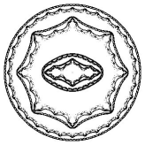
Figure 1: The Julia set of $G=\langle g_{1}^{2},g_{2}^{2}\rangle.$

In [29, 30, 28, 19, 35, 31], we obtain many examples of postcritically bounded polynomial semigroups with many additional properties. In fact, several systematic ways to give such examples are found in those papers.

4 Tools

In this section, we recall some fundamental tools to prove the main results.

Let $G$ be a rational semigroup. Then, for each $g\in G$, $g(F(G))\subset F(G),g^{-1}(J(G))\subset J(G).$ If $G$ is generated by a compact family $\Lambda$ of Rat, then $J(G)=\bigcup_{h\in\Lambda}h^{-1}(J(G))$ (this is called backward self-similarity). If $\sharp J(G)\geq 3$, then $J(G)$ is a perfect set and $J(G)$ is equal to the closure of the set of repelling cycles of elements of $G$. We set $E(G):=\{z\in\hat{\mathbb{C}}\mid\sharp\bigcup_{g\in G}g^{-1}(\{z\})<\infty\}.$ If $\sharp J(G)\geq 3$, then $\sharp E(G)\leq 2$ and for each $z\in J(G)\setminus E(G)$, $J(G)=\overline{\bigcup_{g\in G}g^{-1}(\{z\})}.$ If $\sharp J(G)\geq 3$, then $J(G)$ is the smallest set in $\{\emptyset\neq K\subset\hat{\mathbb{C}}\mid K\mbox{ is compact},\forall g\in G,g(K)\subset K\}.$ For more details on these properties of rational semigroups, see [11, 17, 10, 22]. For the dynamics of postcritically bounded polynomial semigroups, see [29, 30, 19]. If $f:X\times\hat{\mathbb{C}}\rightarrow X\times\hat{\mathbb{C}}$ is a polynomial skew product such that $\deg(f_{x})\geq 2$ for each $x\in X$ and such that $\pi_{\hat{\mathbb{C}}}(P(f))\setminus\{\infty\}$ is bounded in $\mathbb{C}$, then for each $x\in X$, $J_{x}(f)$ is connected ([30, Lemma 3.6]). For some fundamental properties of skew products, see [23, 25, 30].

5 Proofs

In this section, we give the proofs of the main results.

5.1 Proofs of the results in 3.1

In this section, we prove results in section 3.1.

To prove results in 3.1, we need the following notations and lemmas.

Definition 5.1 ([23]).

Let $f:X\times\hat{\mathbb{C}}\rightarrow X\times\hat{\mathbb{C}}$ be a rational skew product over $g:X\rightarrow X.$ Let $N\in\mathbb{N}.$ We say that a point $(x_{0},y_{0})\in X\times\hat{\mathbb{C}}$ belongs to $SH_{N}(f)$ if there exists a neighborhood $U$ of $x_{0}$ in $X$ and a positive number $\delta$ such that, for any $x\in U$, any $n\in\mathbb{N}$, any $x_{n}\in g^{-n}(x)$, and any connected component $V$ of $(f_{x_{n},n})^{-1}(B(y_{0},\delta))$, we have $\deg(f_{x_{n},n}:V\rightarrow B(y_{0},\delta))\leq N.$ Moreover, we set $UH(f):=(X\times\hat{\mathbb{C}})\setminus\cup_{N\in\mathbb{N}}SH_{N}(f).$ We say that $f$ is semi-hyperbolic (along fibers) if $UH(f)\subset\tilde{F}(f).$

Remark 5.2.

Under the above notation, we have $UH(f)\subset P(f).$

Remark 5.3.

Let $\Gamma$ be a compact subset of Rat and let $f:\Gamma^{\mathbb{N}}\times\hat{\mathbb{C}}\rightarrow\Gamma^{\mathbb{N}}\times\hat{\mathbb{C}}$ be the skew product associated with $\Gamma.$ Let $G$ be the rational semigroup generated by $\Gamma.$ Then, by [30, Remark 2.12], $f$ is semi-hyperbolic if and only if $G$ is semi-hyperbolic. Similarly, $f$ is hyperbolic if and only if $G$ is hyperbolic.

For a point $z\in\mathbb{C}$ and a number $r>0$, we set $D(z,r):=\{z\in\mathbb{C}\mid|y-z|<r\}.$

Lemma 5.4.

Let $f:X\times\hat{\mathbb{C}}\rightarrow X\times\hat{\mathbb{C}}$ be a polynomial skew product over $g:X\rightarrow X$ such that for each $\omega\in X$, we have $d(\omega)\geq 2.$ Let $x\in X$ and $y_{0}\in F_{x}(f)$. Suppose that there exists a strictly increasing sequence $\{n_{j}\}_{j\in\mathbb{N}}$ of positive integers such that the sequence $\{f_{x,n_{j}}\}_{j\in\mathbb{N}}$ converges to a non-constant map around $y_{0}$, and such that $\lim_{j\rightarrow\infty}f^{n_{j}}(x,y_{0})$ exists. We set $(x_{\infty},y_{\infty}):=\lim_{j\rightarrow\infty}f^{n_{j}}(x,y_{0}).$ Then, there exists a non-empty bounded open set $V$ in $\mathbb{C}$ and a number $k\in\mathbb{N}$ such that $\{x_{\infty}\}\times\partial V\subset\tilde{J}(f)\cap UH(f)\subset\tilde{J}(f)\cap P(f)$, and such that for each $j$ with $j\geq k$, $f_{x,n_{j}}(y_{0})\in V.$

Proof.

We set

$$V:=\{y\in\hat{\mathbb{C}}\mid\exists\epsilon>0,\lim_{i\rightarrow\infty}\sup_{j>i}\sup_{d(\xi,y)\leq\epsilon}d(f_{g^{n_{i}}(x),n_{j}-n_{i}}(\xi),\xi)=0\}.$$

Then, by [23, Lemma 2.13], we have $\{x_{\infty}\}\times\partial V\subset\tilde{J}(f)\cap UH(f)\subset\tilde{J}(f)\cap P(f).$ Moreover, since for each $x\in X$, $f_{x,1}$ is a polynomial with $d(x)\geq 2$, [30, Lemma 3.4(4)] implies that there exists a ball $B$ around $\infty$ such that $B\subset\hat{\mathbb{C}}\setminus V.$

From the assumption, there exists a number $a>0$ and a non-constant map $\varphi:D(y_{0},a)\rightarrow\hat{\mathbb{C}}$ such that $f_{x,n_{j}}\rightarrow\varphi$ as $j\rightarrow\infty$, uniformly on $D(y_{0},a).$ Hence, $d(f_{x,n_{j}}(y),f_{x,n_{i}}(y))\rightarrow 0$ as $i,j\rightarrow\infty$, uniformly on $D(y_{0},a).$ Moreover, since $\varphi$ is not constant, there exists a positive number $\epsilon$ such that, for each large $i$, $f_{x,n_{i}}(D(y_{0},a))\supset D(y_{\infty},\epsilon).$ Therefore, it follows that $d(f_{g^{n_{i}}(x),n_{j}-n_{i}}(\xi),\xi)\rightarrow 0$ as $i,j\rightarrow\infty$ uniformly on $D(y_{\infty},\epsilon).$ Thus, $y_{\infty}\in V.$ Hence, there exists a number $k\in\mathbb{N}$ such that, for each $j\geq k$, $f_{x,n_{j}}(y_{0})\in V.$ Therefore, we have proved Lemma 5.4. ∎

Remark 5.5.

In [23, Lemma 2.13] and [25, Theorem 2.6], the sequence $(n_{j})$ of positive integers should be strictly increasing.

Lemma 5.6.

Let $\Gamma$ be a non-empty compact subset of Poly${}_{\deg\geq 2}.$ Let $f:\Gamma^{\mathbb{N}}\times\hat{\mathbb{C}}\rightarrow\Gamma^{\mathbb{N}}\times\hat{\mathbb{C}}$ be the skew product associated with $\Gamma.$ Let $G$ be the polynomial semigroup generated by $\Gamma.$ Let $\gamma\in\Gamma^{\mathbb{N}}$. Let $y_{0}\in F_{\gamma}(f)$ and suppose that there exists a strictly increasing sequence $\{n_{j}\}_{j\in\mathbb{N}}$ of positive integers such that $\{f_{\gamma,n_{j}}\}_{j\in\mathbb{N}}$ converges to a non-constant map around $y_{0}.$ Moreover, suppose that $G\in{\cal G}.$ Then, there exists a number $j\in\mathbb{N}$ such that $f_{\gamma,n_{j}}(y_{0})\in$ int$(\hat{K}(G)).$

Proof.

By Lemma 5.4, there exists a bounded open set $V$ in $\mathbb{C}$, a point $\gamma_{\infty}\in\Gamma^{\mathbb{N}}$, and a number $j\in\mathbb{N}$ such that $\{\gamma_{\infty}\}\times\partial V\subset\tilde{J}(f)\cap P(f)$, and such that $f_{\gamma,n_{j}}(y_{0})\in V.$ Then, we have $\partial V\subset P^{\ast}(G).$ Since $g(P^{\ast}(G))\subset P^{\ast}(G)$ for each $g\in G$, the maximum principle implies that $V\subset$ int$(\hat{K}(G)).$ Hence, $f_{\gamma,n_{j}}(y_{0})\in$ int$(\hat{K}(G)).$ Therefore, we have proved Lemma 5.6. ∎

We now demonstrate statements 1 and 2 of Theorem 3.11.
Proof of statements 1 and 2 of Theorem 3.11: First, we will show the following claim.
Claim 1. Let $\gamma\in R(\Gamma,\Gamma\setminus\Gamma_{\min}).$ Then, for any point $y_{0}\in F_{\gamma}(f)$, there exists no non-constant limit function of $\{f_{\gamma,n}\}_{n\in\mathbb{N}}$ around $y_{0}.$

To show this claim, suppose that there exists a strictly increasing sequence $\{n_{j}\}_{j\in\mathbb{N}}$ of positive integers such that $f_{\gamma,n_{j}}$ tends to a non-constant map as $j\rightarrow\infty$ around $y_{0}.$ We consider the following two cases: Case (i): $\Gamma\setminus\Gamma_{\min}$ is compact. Case (ii): $\Gamma\setminus\Gamma_{\min}$ is not compact. Suppose that we have Case (i). Since $G\in{\cal G}$, Lemma 5.6 implies that there exists a number $k\in\mathbb{N}$ such that $f_{\gamma,n_{k}}(y_{0})\in$ int$(\hat{K}(G)).$ Hence, we get that the sequence $\{f_{\sigma^{n_{k}}(\gamma),n_{k+j}-n_{k}}\}_{j\in\mathbb{N}}$ converges to a non-constant map around the point $y_{1}:=f_{\gamma,n_{k}}(y_{0})\in$ int$(\hat{K}(G)).$ However, since we are assuming that $\Gamma\setminus\Gamma_{\min}$ is compact, [29, Theorem 2.20.5(b)] implies that $\cup_{h\in\Gamma\setminus\Gamma_{\min}}h(\hat{K}(G))$ is a compact subset of int$(\hat{K}(G))$, which implies that if we take the hyperbolic metric for each connected component of int$(\hat{K}(G))$, then there exists a constant $0<c<1$ such that for each $z\in$ int$(\hat{K}(G))$ and each $h\in\Gamma\setminus\Gamma_{\min}$, we have $\|h^{\prime}(z)\|\leq c$, where $\|h^{\prime}(z)\|$ denotes the norm of the derivative of $h$ at $z$ measured from the hyperbolic metric on the connected component $W_{1}$ of int$(\hat{K}(G))$ containing $z$ to that of the connected component $W_{2}$ of int$(\hat{K}(G))$ containing $h(z).$ This leads to a contradiction, since we have that $\gamma\in R(\Gamma,\Gamma\setminus\Gamma_{\min})$ and the sequence $\{f_{\sigma^{n_{k}}(\gamma),n_{k+j}-n_{k}}\}_{j\in\mathbb{N}}$ converges to a non-constant map around the point $y_{1}\in$ int$(\hat{K}(G)).$ We now suppose that we have Case (ii). Then, combining the arguments in Case (i) and [29, Theorem 2.20.5(b), Proposition 2.33], we again obtain a contradiction. Hence, we have shown Claim 1.

Next, let $S$ be a non-empty compact subset of $\Gamma\setminus\Gamma_{\min}$ and let $\gamma\in R(\Gamma,S).$ We show the following claim.
Claim 2. For each point $y_{0}$ in each bounded component of $F_{\gamma}(f)$, there exists a number $n\in\mathbb{N}$ such that $f_{\gamma,n}(y_{0})\in$ int$(\hat{K}(G)).$

To show this claim, we suppose that there exists no $n\in\mathbb{N}$ such that $f_{\gamma,n}(y_{0})\in$ int$(\hat{K}(G))$. By Claim 1, $\{f_{\gamma,n}\}_{n\in\mathbb{N}}$ has only constant limit functions around $y_{0}.$ Moreover, if a point $w_{0}\in\mathbb{C}$ is a constant limit function of $\{f_{\gamma,n}\}_{n\in\mathbb{N}}$, then since $G\in{\cal G}$, [30, Lemma 3.13] implies that we must have that $w_{0}\in P^{\ast}(G)\subset\hat{K}(G).$ Since we are assuming that there exists no $n\in\mathbb{N}$ such that $f_{\gamma,n}(y_{0})\in$ int$(\hat{K}(G))$, it follows that $w_{0}\in\partial\hat{K}(G).$ Combining this with [29, Theorem 2.20.2] we deduce that $w_{0}\in\partial\hat{K}(G)\subset J_{\min}.$ From this argument, we get that

$$d(f_{\gamma,n}(y_{0}),J_{\min})\rightarrow 0,\mbox{ as }n\rightarrow\infty.$$ (1)

However, since $\gamma$ belongs to $R(\Gamma,S)$, the above (1) implies that the sequence $\{f_{\gamma,n}(y_{0})\}_{n\in\mathbb{N}}$ accumulates in the compact set $\cup_{h\in S}h^{-1}(J_{\min})$, which is apart from $J_{\min}$, by [29, Theorem 2.20.5(b)]. This contradicts (1). Hence, we have shown that Claim 2 holds.

Next, we show the following claim.
Claim 3. There exists exactly one bounded component $U_{\gamma}$ of $F_{\gamma}(f).$

To show this claim, we take an element $h\in\Gamma_{\min}$ (note that $\Gamma_{\min}\neq\emptyset$, by Proposition 2.10). We write the element $\gamma$ as $\gamma=(\gamma_{1},\gamma_{2},\ldots).$ For any $l\in\mathbb{N}$ with $l\geq 2$, let $s_{l}\in\mathbb{N}$ be an integer with $s_{l}>l$ such that $\gamma_{s_{l}}\in S.$ We may assume that for each $l\in\mathbb{N}$, $s_{l}<s_{l+1}.$ For each $l\in\mathbb{N}$, let $\gamma^{l}:=(\gamma_{1},\gamma_{2},\ldots,\gamma_{s_{l}-1},h,h,h,\ldots)\in\Gamma^{\mathbb{N}}$ and $\tilde{\gamma}^{l}:=\sigma^{s_{l}-1}(\gamma)=(\gamma_{s_{l}},\gamma_{s_{l}+1},\ldots)\in\Gamma^{\mathbb{N}}.$ Moreover, let $\rho:=(h,h,h,\ldots)\in\Gamma^{\mathbb{N}}.$ Since $h\in\Gamma_{\min}$, we have

$$J_{\rho}(f)=J(h)\subset J_{\min}.$$ (2)

Moreover, since $\gamma_{s_{l}}$ does not belong to $\Gamma_{\min}$, combining it with [29, Theorem 2.20.5(b)], we obtain $\gamma_{s_{l}}^{-1}(J(G))\cap J_{\min}=\emptyset.$ Hence, we have that for each $l\in\mathbb{N}$,

$$J_{\tilde{\gamma}^{l}}(f)=\gamma_{s_{l}}^{-1}(J_{\sigma^{s_{l}}(\gamma)}(f))\subset\gamma_{s_{l}}^{-1}(J(G))\subset\hat{\mathbb{C}}\setminus J_{\min}.$$ (3)

Combining (2), (3), and [30, Lemma 3.9] we obtain

$$J_{\rho}(f)<J_{\tilde{\gamma}^{l}}(f),$$ (4)

which implies

$$J_{\gamma^{l}}(f)=(f_{\gamma,s_{l}-1})^{-1}(J_{\rho}(f))<(f_{\gamma,s_{l}-1})^{-1}(J_{\tilde{\gamma}^{l}}(f))=J_{\gamma}(f).$$ (5)

From [30, Lemma 3.9] and (5), it follows that there exists a bounded component $U_{\gamma}$ of $F_{\gamma}(f)$ such that for each $l\in\mathbb{N}$ with $l\geq 2$,

$$J_{\gamma^{l}}(f)\subset U_{\gamma}.$$ (6)

We now suppose that there exists a bounded component $V$ of $F_{\gamma}(f)$ with $V\neq U_{\gamma}$, and we will deduce a contradiction. Under the above assumption, we take a point $y\in V.$ Then, by Claim 2, we get that there exists a number $l\in\mathbb{N}$ such that $f_{\gamma,l}(y)\in$ int$(\hat{K}(G)).$ Since $s_{l}>l$, we obtain $f_{\gamma,s_{l}-1}(y)\in$ int$(\hat{K}(G))\subset K(h)$, where, $h\in\Gamma_{\min}$ is the element which we have taken before. By (4), we have that there exists a bounded component $B$ of $F_{\tilde{\gamma}^{l}}(f)$ containing $K(h).$ Hence, we have $f_{\gamma,s_{l}-1}(y)\in B.$ Since the map $f_{\gamma,s_{l}-1}:V\rightarrow B$ is surjective, it follows that $V\cap\left((f_{\gamma,s_{l}-1})^{-1}(J(h))\right)\neq\emptyset.$ Combining this with $(f_{\gamma,s_{l}-1})^{-1}(J(h))=(f_{\gamma^{l},s_{l}-1})^{-1}(J(h))=J_{\gamma^{l}}(f)$, we obtain $V\cap J_{\gamma^{l}}(f)\neq\emptyset.$ However, this leads to a contradiction, since we have (6) and $U_{\gamma}\cap V=\emptyset.$ Hence, we have shown Claim 3.

Next, we show the following claim.
Claim 4. We have $\partial U_{\gamma}=\partial A_{\gamma}(f)=J_{\gamma}(f).$

To show this claim, since $U_{\gamma}=\mbox{int}(K_{\gamma}(f))$, [30, Lemma 3.4(5)] implies that $\partial U_{\gamma}=J_{\gamma}(f).$ Moreover, by [30, Lemma 3.4(4)] we have $\partial A_{\gamma}(f)=J_{\gamma}(f).$ Thus, we have shown Claim 4.

We now show the following claim.
Claim 5. We have $\hat{J}_{\gamma}(f)=J_{\gamma}(f)$ and the map $\omega\mapsto J_{\omega}(f)$ is continuous at $\gamma$ with respect to the Hausdorff metric in the space of non-empty compact subsets of $\hat{\mathbb{C}}.$

To show this claim, suppose that there exists a point $z$ with $z\in\hat{J}_{\gamma}(f)\setminus J_{\gamma}(f).$ Since $\hat{J}_{\gamma}(f)\setminus J_{\gamma}(f)$ is included in the union of bounded components of $F_{\gamma}(f)$, combining it with Claim 2, we get that there exists a number $n\in\mathbb{N}$ such that $f_{\gamma,n}(z)\in$ int$(\hat{K}(G))\subset F(G).$ However, since $z\in\hat{J}_{\gamma}(f)$, we must have that $f_{\gamma,n}(z)=\pi_{\hat{\mathbb{C}}}(f_{\gamma}^{n}(z))\in\pi_{\hat{\mathbb{C}}}(\tilde{J}(f))=J(G).$ This is a contradiction. Hence, we obtain $\hat{J}_{\gamma}(f)=J_{\gamma}(f).$ Combining this with [30, Lemma 3.4(2)], it follows that $\omega\mapsto J_{\omega}(f)$ is continuous at $\gamma.$ Therefore, we have shown Claim 5.

Combining all Claims $1,\ldots,5$, it follows that statements 1, 2(a), 2(b) and 2(c) of Theorem 3.11 hold.

We now show statement 2(d). Let $\gamma\in R(\Gamma,S)$ be an element. Suppose that $m_{2}(J_{\gamma}(f))>0$, where $m_{2}$ denotes the $2$-dimensional Lebesgue measure. Then, there exists a Lebesgue density point $b\in J_{\gamma}(f)$ so that

$$\lim_{s\rightarrow 0}\frac{m_{2}\left(D(b,s)\cap J_{\gamma}(f)\right)}{m_{2}(D(b,s))}=1.$$ (7)

Since $\gamma$ belongs to $R(\Gamma,S)$, there exists an element $\gamma_{\infty}\in S$ and a sequence $\{n_{j}\}_{j\in\mathbb{N}}$ of positive integers such that $n_{j}\rightarrow\infty$ and $\gamma_{n_{j}}\rightarrow\gamma_{\infty}$ as $j\rightarrow\infty$, and such that for each $j\in\mathbb{N}$, we have $\gamma_{n_{j}}\in S.$ We set $b_{j}:=f_{\gamma,n_{j}-1}(b)$, for each $j\in\mathbb{N}.$ We may assume that there exists a point $a\in\mathbb{C}$ such that $b_{j}\rightarrow a$ as $j\rightarrow\infty.$ Since $\gamma_{n_{j}}(b_{j})=f_{\gamma,n_{j}}(b)=\pi_{\hat{\mathbb{C}}}(f_{\gamma}^{n_{j}}(\gamma,b))\in\pi_{\hat{\mathbb{C}}}(\tilde{J}(f))=J(G)$, we obtain $a\in\gamma_{\infty}^{-1}(J(G)).$ Moreover, by [29, Theorem 2.20.5(b)], we obtain

$$a\in\gamma_{\infty}^{-1}(J(G))\subset\mathbb{C}\setminus J_{\min}.$$ (8)

Combining this with [29, Theorem 2.20.2], it follows that $r:=\inf\{|a-b|\mid b\in P^{\ast}(G)\}>0.$ Let $\epsilon$ be arbitrary number with $0<\epsilon<\frac{r}{10}.$ We may assume that for each $j\in\mathbb{N}$, we have $b_{j}\in D(a,\frac{\epsilon}{2}).$ For each $j\in\mathbb{N},$ let $\varphi_{j}$ be the well-defined inverse branch of $f_{\gamma,n_{j}-1}$ on $D(a,r)$ such that $\varphi_{j}(b_{j})=b.$ Let $V_{j}:=\varphi_{j}(D(b_{j},r-\epsilon))$, for each $j\in\mathbb{N}.$ We now show the following claim.
Claim 6. diam $V_{j}\rightarrow 0$, as $\j\rightarrow\infty.$

To show this claim, suppose that this is not true. Then, there exists a strictly increasing sequence $\{j_{k}\}_{k\in\mathbb{N}}$ of positive integers and a positive constant $\kappa$ such that for each $k\in\mathbb{N}$, diam $V_{j_{k}}\geq\kappa.$ From the Koebe distortion theorem, it follows that there exists a positive constant $c_{0}$ such that for each $k\in\mathbb{N}$, $V_{j_{k}}\supset D(b,c_{0}).$ This implies that for each $k\in\mathbb{N}$, $f_{\gamma,v_{k}}(D(b,c_{0}))\subset D(b_{j_{k}},r-\epsilon)$, where $v_{k}:=n_{j_{k}}-1.$ Since $v_{k}\rightarrow\infty$ as $k\rightarrow\infty$ and $f_{\gamma^{\prime},n}|_{F_{\infty}(G)}\rightarrow\infty$ for any $\gamma^{\prime}\in\Gamma^{\mathbb{N}}$, it follows that for any $n\in\mathbb{N}$, $f_{\gamma,n}(D(b,c_{0}))\subset\hat{\mathbb{C}}\setminus F_{\infty}(G)$, which implies that $b\in F_{\gamma}(f).$ However, it contradicts $b\in J_{\gamma}(f).$ Hence, Claim 6 holds.

Combining the Koebe distortion theorem and Claim 6, we see that there exist a constant $K>0$ and two sequences $\{r_{j}\}_{j\in\mathbb{N}}$ and $\{R_{j}\}_{j\in\mathbb{N}}$ of positive numbers such that $K\leq\frac{r_{j}}{R_{j}}<1$ and $D(b,r_{j})\subset V_{j}\subset D(b,R_{j})$ for each $j\in\mathbb{N}$, and such that $R_{j}\rightarrow 0$ as $j\rightarrow\infty$. From (7), it follows that

$$\lim_{j\rightarrow\infty}\frac{m_{2}\left(V_{j}\cap F_{\gamma}(f)\right)}{m_{2}(V_{j})}=0.$$ (9)

For each $j\in\mathbb{N}$, let $\psi_{j}:D(0,1)\rightarrow\varphi_{j}(D(a,r))$ be a biholomorphic map such that $\psi_{j}(0)=b.$ Then, there exists a constant $0<c_{1}<1$ such that for each $j\in\mathbb{N}$,

$$\psi_{j}^{-1}(V_{j})\subset D(0,c_{1}).$$ (10)

Combining this with (9) and the Koebe distortion theorem, it follows that

$$\lim_{j\rightarrow\infty}\frac{m_{2}\left(\psi_{j}^{-1}(V_{j}\cap F_{\gamma}(f))\right)}{m_{2}(\psi_{j}^{-1}(V_{j}))}=0.$$ (11)

Since $\varphi_{j}^{-1}(\psi_{j}(D(0,1)))\subset D(a,r)$ for each $j\in\mathbb{N}$, combining (10) and Cauchy’s formula yields that there exists a constant $c_{2}>0$ such that for any $j\in\mathbb{N}$,

$$|(f_{\gamma,n_{j}-1}\circ\psi_{j})^{\prime}(z)|\leq c_{2}\ \mbox{ on }\psi_{j}^{-1}(V_{j}).$$ (12)

Combining (11) and (12), we obtain

$$\frac{m_{2}\left(D(b_{j},r-\epsilon)\cap F_{\sigma^{n_{j}-1}(\gamma)}(f)\right)}{m_{2}(D(b_{j},r-\epsilon))}=\frac{m_{2}\left((f_{\gamma,n_{j}-1}\circ\psi_{j})(\psi_{j}^{-1}(V_{j}\cap F_{\gamma}(f)))\right)}{m_{2}(D(b_{j},r-\epsilon))}$$

$$=\frac{\int_{\psi_{j}^{-1}(V_{j}\cap F_{\gamma}(f))}|(f_{\gamma,n_{j}-1}\circ\psi_{j})^{\prime}(z)|^{2}\ dm_{2}(z)}{m_{2}(\psi_{j}^{-1}(V_{j}))}\cdot\frac{m_{2}(\psi_{j}^{-1}(V_{j}))}{m_{2}(D(b_{j},r-\epsilon))}\rightarrow 0,$$

as $j\rightarrow\infty.$ Hence, we obtain

$$\lim_{j\rightarrow\infty}\frac{m_{2}\left(D(b_{j},r-\epsilon)\cap J_{\sigma^{n_{j}-1}(\gamma)}(f)\right)}{m_{2}(D(b_{j},r-\epsilon))}=1.$$

Since $J_{\sigma^{n_{j}-1}(\gamma)}(f)\subset J(G)$ for each $j\in\mathbb{N}$, and $b_{j}\rightarrow a$ as $j\rightarrow\infty$, it follows that

$$\frac{m_{2}(D(a,r-\epsilon)\cap J(G))}{m_{2}(D(a,r-\epsilon))}=1.$$

This implies that $D(a,r-\epsilon)\subset J(G).$ Since this is valid for any $\epsilon$, we must have that $D(a,r)\subset J(G).$ It follows that the point $a$ belongs to a connected component $J$ of $J(G)$ such that $J\cap P^{\ast}(G)\neq\emptyset.$ However, [29, Theorem 2.20.2] implies that the component $J$ is equal to $J_{\min}$, which leads to a contradiction since we have (8). Hence, we have shown statement 2(d) of Theorem 3.11.

Therefore, we have proved statements 1 and 2 of Theorem 3.11. ∎

We now demonstrate statement 3 of Theorem 3.11.
Proof of statement 3 of Theorem 3.11: First, we remark that the subset $W_{S,p}$ of $\Gamma^{\mathbb{N}}$ is a $\sigma$-invariant compact set. Hence, $\overline{f}:W_{S,p}\times\hat{\mathbb{C}}\rightarrow W_{S,p}\times\hat{\mathbb{C}}$ is a polynomial skew product over $\sigma:W_{S,p}\rightarrow W_{S,p}.$ Suppose that $\tilde{J}(\overline{f})\cap P(\overline{f})\neq\emptyset$ and let $(\gamma,y)\in\tilde{J}(\overline{f})\cap P(\overline{f})$ be a point. Then, since the point $\gamma=(\gamma_{1},\gamma_{2},\ldots)$ belongs to $W_{S,p}$, there exists a number $j\in\mathbb{N}$ such that $\gamma_{j}\in S.$ Combining this with the condition that $G\in{\cal G}_{dis}$ and [29, Theorem 2.20.5(b), Theorem 2.20.2], we have $\gamma_{j}^{-1}(J(G))\subset\mathbb{C}\setminus\hat{K}(G)\subset\mathbb{C}\setminus P(G).$ Moreover, we have that $\pi_{\hat{\mathbb{C}}}(\overline{f}_{\gamma}^{j-1}(\gamma,y))=\pi_{\hat{\mathbb{C}}}(f_{\gamma}^{j-1}(\gamma,y))\in J_{\sigma^{j-1}(\gamma)}(f)=\gamma_{j}^{-1}\left(J_{\sigma^{j}(\gamma)}(f)\right)\subset\gamma_{j}^{-1}(J(G)).$ Hence, we obtain

$$\pi_{\hat{\mathbb{C}}}(\overline{f}_{\gamma}^{j-1}(\gamma,y))\in\mathbb{C}\setminus P(G).$$ (13)

However, since $(\gamma,y)\in P(\overline{f})$, we have that $\pi_{\hat{\mathbb{C}}}(\overline{f}_{\gamma}^{j-1}(\gamma,y))\in\pi_{\hat{\mathbb{C}}}(P(\overline{f}))\subset P(G)$, which contradicts (13). Hence, we must have that $\tilde{J}(\overline{f})\cap P(\overline{f})=\emptyset.$ Therefore, $\overline{f}:W_{S,p}\times\hat{\mathbb{C}}\rightarrow W_{S,p}\times\hat{\mathbb{C}}$ is a hyperbolic polynomial skew product over the shift map $\sigma:W_{S,p}\rightarrow W_{S,p}.$

Combining this with statement 2(a) of Theorem 3.11 and [30, Theorem 4.1] we conclude that there exists a constant $K_{S,p}\geq 1$ such that for each $\gamma\in W_{S,p},\ J_{\gamma}(\overline{f})$ is a $K_{S,p}$-quasicircle. Moreover, by statement 2(c) of Theorem 3.11, we have $J_{\gamma}(\overline{f})=J_{\gamma}(f)=\hat{J}_{\gamma}(f).$

Hence, we have shown statement 3 of Theorem 3.11. ∎
We now demonstrate Theorem 3.13.
Proof of Theorem 3.13: Let $\gamma\in R(\Gamma,\Gamma\setminus\Gamma_{\min})$ and $y\in$ int$(K_{\gamma}(f)).$ Combining statement 1 of Theorem 3.11 and [23, Lemma 1.10], we obtain $\liminf_{n\rightarrow\infty}$ $d(f_{\gamma,n}(y),$ $J(G))>0.$ Combining this with [30, Lemma 3.13] and statement 1 of Theorem 3.11, we see that there exists a point $a\in P^{\ast}(G)\cap F(G)$ such that $\liminf_{n\rightarrow\infty}d(f_{\gamma,n}(y),a)=0.$ Since $P^{\ast}(G)\cap F(G)\subset$ int$(\hat{K}(G))$ (which follows from the condition that $G\in{\cal G}$), it follows that there exists a positive integer $l$ such that $f_{\gamma,l}(y)\in\mbox{int}(\hat{K}(G)).$ Combining this and the same method as that in the proof of Claim 3 in the proof of statements 1 and 2 of Theorem 3.11, we get that there exists exactly one bounded component $U_{\gamma}$ of $F_{\gamma}(f).$ Combining it with [30, Proposition 4.6], it follows that $J_{\gamma}(f)$ is a Jordan curve. Moreover, by [23, Theorem 2.14-(4)], we have $\hat{J}_{\gamma}(f)=J_{\gamma}(f).$

Thus, we have proved Theorem 3.13. ∎

We now demonstrate Theorem 3.14.

Proof of Theorem 3.14: Let $V$ be an open set with $J(G)\cap V\neq\emptyset.$ We may assume that $V$ is connected. Then, by [11, Corollary 3.1] there exists an element $\alpha_{1}\in G$ such that $J(\alpha_{1})\cap V\neq\emptyset.$ Since we have $G\in{\cal G}_{dis}$, [29, Theorem 2.1] implies that there exists an element $\alpha_{2}\in G$ such that no connected component $J$ of $J(G)$ satisfies $J(\alpha_{1})\cup J(\alpha_{2})\subset J.$ Hence, we have $\langle\alpha_{1},\alpha_{2}\rangle\in{\cal G}_{dis}.$ Since $J(\alpha_{1})\cap V\neq\emptyset$, combining this with [30, Lemma 3.4(2)] we get that there exists an $l_{0}\in\mathbb{N}$ such that for each $l$ with $l\geq l_{0}$, we have $J(\alpha_{2}\alpha_{1}^{l})\cap V\neq\emptyset.$ Moreover, since no connected component $J$ of $J(G)$ satisfies $J(\alpha_{1})\cup J(\alpha_{2})\subset J$, [30, Lemma 3.4(2)] implies that there exists an $l_{1}\in\mathbb{N}$ such that for each $l$ with $l\geq l_{1}$, $J(\alpha_{2}\alpha_{1}^{l})\cap J(\alpha_{1}\alpha_{2}^{l})=\emptyset.$ We fix an $l\in\mathbb{N}$ with $l\geq\max\{l_{0},l_{1}\}.$ We now show the following claim.
Claim 1. The semigroup $H_{0}:=\langle\alpha_{2}\alpha_{1}^{l},\alpha_{1}\alpha_{2}^{l}\rangle$ is hyperbolic, and for the skew product $\tilde{f}:\Gamma^{\mathbb{N}}_{0}\times\hat{\mathbb{C}}\rightarrow\Gamma^{\mathbb{N}}_{0}\times\hat{\mathbb{C}}$ associated with $\Gamma_{0}=\{\alpha_{2}\alpha_{1}^{l},\alpha_{1}\alpha_{2}^{l}\}$, there exists a constant $K\geq 1$ such that for any $\gamma\in\Gamma^{\mathbb{N}}_{0}$, $J_{\gamma}(\tilde{f})$ is a $K$-quasicircle.

To show this claim, applying statement 3 of Theorem 3.11 with $\Gamma=\{\alpha_{1},\alpha_{2}\},S=\Gamma\setminus\Gamma_{\min},$ and $p=2l+1$, we see that the polynomial skew product $\overline{f}:W_{S,2l+1}\times\hat{\mathbb{C}}\rightarrow W_{S,2l+1}\times\hat{\mathbb{C}}$ over $\sigma:W_{S,2l+1}\rightarrow W_{S,2l+1}$ is hyperbolic, and that there exists a constant $K\geq 1$ such that for each $\gamma\in W_{S,2l+1}$, $J_{\gamma}(\overline{f})$ is a $K$-quasicircle. Moreover, combining the hyperbolicity of $\overline{f}$ above and Remark 5.3, we see that the semigroup $H_{1}$ generated by the family $\{\alpha_{j_{1}}\circ\cdots\circ\alpha_{j_{l+1}}\mid 1\leq\exists k_{1}\leq l+1\mbox{ with }j_{k_{1}}=1,1\leq\exists k_{2}\leq l+1\mbox{ with }j_{k_{2}}=2\}$ is hyperbolic. Hence, the semigroup $H_{0}$, which is a subsemigroup of $H_{1}$, is hyperbolic. Therefore, Claim 1 holds.

We now show the following claim.
Claim 2. We have either $J(\alpha_{2}\alpha_{1}^{l})<J(\alpha_{1}\alpha_{2}^{l})$, or $J(\alpha_{1}\alpha_{2}^{l})<J(\alpha_{2}\alpha_{1}^{l}).$

To show this claim, since $J(\alpha_{2}\alpha_{1}^{l})\cap J(\alpha_{1}\alpha_{2}^{l})=\emptyset$ and $H_{0}\in{\cal G}$, combining these with [30, Lemma 3.9], we obtain Claim 2.

By Claim 2, we have the following two cases.
Case 1. $J(\alpha_{2}\alpha_{1}^{l})<J(\alpha_{1}\alpha_{2}^{l}).$
Case 2. $J(\alpha_{1}\alpha_{2}^{l})<J(\alpha_{2}\alpha_{1}^{l}).$

We may assume that we have Case 1 (when we have Case 2, we can show all statements of our theorem, using the same method as below). Let $A:=K(\alpha_{1}\alpha_{2}^{l})\setminus$ int$(K(\alpha_{2}\alpha_{1}^{l})).$ By Claim 1, we have that $J(\alpha_{1}\alpha_{2}^{l})$ and $J(\alpha_{2}\alpha_{1}^{l})$ are quasicircles. Moreover, since $H_{0}\in{\cal G}_{dis}$ and $H_{0}$ is hyperbolic, we must have $P^{\ast}(H_{0})\subset$ int$(K(\alpha_{2}\alpha_{1}^{l})).$ Therefore, it follows that if we take a small open neighborhood $U$ of $A$, then there exists a number $n\in\mathbb{N}$ such that, setting $h_{1}:=(\alpha_{2}\alpha_{1}^{l})^{n}$ and $h_{2}:=(\alpha_{1}\alpha_{2}^{l})^{n}$, we have that

$$h_{1}^{-1}(\overline{U})\cup h_{2}^{-1}(\overline{U})\subset U\mbox{ and }h_{1}^{-1}(\overline{U})\cap h_{2}^{-1}(\overline{U})=\emptyset.$$ (14)

Moreover, combining [30, Lemma 3.4(2)] and that $J(h_{1})\cap V\neq\emptyset$, we get that there exists a $k\in\mathbb{N}$ such that $J(h_{2}h_{1}^{k})\cap V\neq\emptyset.$ We set $g_{1}:=h_{1}^{k+1}$ and $g_{2}:=h_{2}h_{1}^{k}.$ Moreover, we set $H:=\langle g_{1},g_{2}\rangle.$ Since $H$ is a subsemigroup of $H_{0}$ and $H_{0}$ is hyperbolic, we have that $H$ is hyperbolic. Moreover, (14) implies that $g_{1}^{-1}(\overline{U})\cup g_{2}^{-1}(\overline{U})\subset U$ and $g_{1}^{-1}(\overline{U})\cap g_{2}^{-1}(\overline{U})=\emptyset.$ Hence, we have shown that for the semigroup $H=\langle g_{1},g_{2}\rangle$, statements 1,2, and 3 of Theorem 3.14 hold.

From statement 2 and [11, Corollary 3.2], we obtain $J(H)\subset\overline{U}$ and $g_{1}^{-1}(J(H))\cap g_{2}^{-1}(J(H))=\emptyset.$ Combining this with [22, Lemma 2.4] and [30, Lemma 3.5(2)], it follows that the skew product $f:\Gamma^{\mathbb{N}}_{1}\times\hat{\mathbb{C}}\rightarrow\Gamma^{\mathbb{N}}_{1}\times\hat{\mathbb{C}}$ associated with $\Gamma_{1}=\{g_{1},g_{2}\}$ satisfies that $J(H)$ is equal to the disjoint union of the sets $\{\hat{J}_{\gamma}(f)\}_{\gamma\in\Gamma^{\mathbb{N}}_{1}}.$ Moreover, since $H$ is hyperbolic, [23, Theorem 2.14-(2)] implies that for each $\gamma\in\Gamma_{1}^{\mathbb{N}}$, $\hat{J}_{\gamma}(f)=J_{\gamma}(f).$ In particular, the map $\gamma\mapsto J_{\gamma}(f)$ from $\Gamma^{\mathbb{N}}_{1}$ into the space of non-empty compact sets in $\hat{\mathbb{C}}$, is injective. Since $J_{\gamma}(f)$ is connected for each $\gamma\in\Gamma^{\mathbb{N}}_{1}$ (Claim 1), it follows that for each connected component $J$ of $J(H)$, there exists an element $\gamma\in\Gamma^{\mathbb{N}}_{1}$ such that $J=J_{\gamma}(f).$ Furthermore, by Claim 1, each connected component $J$ of $J(H)$ is a $K$-quasicircle, where $K$ is a constant not depending on $J.$ Moreover, by [23, Theorem 2.14-(4)], the map $\gamma\mapsto J_{\gamma}(f)$ from $\Gamma^{\mathbb{N}}_{1}$ into the space of non-empty compact sets in $\hat{\mathbb{C}}$, is continuous with respect to the Hausdorff metric. Moreover, by Theorem 2.8, $(\{J_{\gamma}(f)\}_{\gamma\in\Gamma^{\mathbb{N}}},\leq)$ is totally ordered. Therefore, we have shown that statements 4(a), 4(b), 4(c), and 4(d) hold for $H=\langle g_{1},g_{2}\rangle$ and $f:\Gamma^{\mathbb{N}}_{1}\times\hat{\mathbb{C}}\rightarrow\Gamma^{\mathbb{N}}_{1}\times\hat{\mathbb{C}}.$

We now show that statement 4(e) holds. Since we are assuming Case 1, Proposition 2.10 implies that $\{h_{1},h_{2}\}_{\min}=\{h_{1}\}.$ Hence $J(g_{1})<J(g_{2}).$ Combining this with Proposition 2.10 and statement 4(b), we obtain

$$J(g_{1})=J_{\min}(H)\mbox{ and }J(g_{2})=J_{\max}(H).$$ (15)

Moreover, since $J(g_{1})=J(\alpha_{2}\alpha_{1}^{l})$, $J(\alpha_{2}\alpha_{1}^{l})\cap V\neq\emptyset$, $J(g_{2})=J(h_{2}h_{1}^{k})$, and $J(h_{2}h_{1}^{k})\cap V\neq\emptyset$, it follows that

$$J_{\min}(H)\cap V\neq\emptyset\mbox{ and }J_{\max}(H)\cap V\neq\emptyset.$$ (16)

Let $\gamma\in\Gamma^{\mathbb{N}}$ be an element such that $J_{\gamma}(f)\cap(J_{\min}(H)\cup J_{\max}(H))=\emptyset.$ By statement 4(b), we obtain

$$J_{\min}(H)<J_{\gamma}(f)<J_{\max}(H).$$ (17)

Since we are assuming $V$ is connected, combining (16) and (17), we obtain $J_{\gamma}(f)\cap V\neq\emptyset.$ Therefore, we have proved that statement 4(e) holds.

We now show that statement 4(f) holds. To show that, let $\omega=(\omega_{1},\omega_{2},\ldots)\in\Gamma^{\mathbb{N}}_{1}$ be an element such that $\sharp(\{j\in\mathbb{N}\mid\omega_{j}=g_{1}\})=\sharp(\{j\in\mathbb{N}\mid\omega_{j}=g_{2}\})=\infty.$ For each $r\in\mathbb{N}$, let $\omega^{r}=(\omega^{r}_{1},\omega^{r}_{2},\ldots)\in\Gamma^{\mathbb{N}}_{1}$ be the element such that $\begin{cases}\omega^{r}_{j}=\omega_{j}\ \ (1\leq j\leq r),\\ \omega^{r}_{j}=g_{1}\ \ (j\geq r+1).\end{cases}$ Moreover, let $\rho^{r}=(\rho^{r}_{1},\rho^{r}_{2},\ldots)\in\Gamma^{\mathbb{N}}_{1}$ be the element such that $\begin{cases}\rho^{r}_{j}=\omega_{j}\ \ (1\leq j\leq r),\\ \rho^{r}_{j}=g_{2}\ \ (j\geq r+1).\end{cases}$ Combining (15) and statements 4(a) and 4(b), we see that for each $r\in\mathbb{N}$, $J(g_{1})<J_{\sigma^{r}(\omega)}(f)<J(g_{2}).$ Hence, by statement 3 of Theorem 2.8, we get that for each $r\in\mathbb{N}$, $(f_{\omega,r})^{-1}(J(g_{1}))<(f_{\omega,r})^{-1}\left(J_{\sigma^{r}(\omega)}(f)\right)<(f_{\omega,r})^{-1}(J(g_{2}))$. Since we have $(f_{\omega,r})^{-1}(J(g_{1}))=J_{\omega^{r}}(f)$, $(f_{\omega,r})^{-1}\left(J_{\sigma^{r}(\omega)}(f)\right)=J_{\omega}(f)$, and $(f_{\omega,r})^{-1}(J(g_{2}))$ $=J_{\rho^{r}}(f)$, it follows that

$$J_{\omega^{r}}(f)<J_{\omega}(f)<J_{\rho^{r}}(f),$$ (18)

for each $r\in\mathbb{N}.$ Moreover, since $\omega^{r}\rightarrow\omega$ and $\rho^{r}\rightarrow\omega$ in $\Gamma^{\mathbb{N}}_{1}$ as $r\rightarrow\infty$, statement 4(d) implies that $J_{\omega^{r}}(f)\rightarrow J_{\omega}(f)$ and $J_{\rho^{r}}(f)\rightarrow J_{\omega}(f)$ as $r\rightarrow\infty$, with respect to the Hausdorff metric. Combining these with (18) and statements 4(b) and 4(c), we get that for any connected component $W$ of $F(H)$, we must have $\partial W\cap J_{\omega}(f)=\emptyset.$ Since $F(G)\subset F(H)$, it follows that for any connected component $W^{\prime}$ of $F(G)$, $\partial W^{\prime}\cap J_{\omega}(f)=\emptyset.$ Therefore, we have shown that statement 4(f) holds.

Thus, we have proved Theorem 3.14. ∎

5.2 Proofs of the results in 3.2

In this section, we demonstrate Theorems 3.18 and 3.19. We need the following notations and lemmas.

Definition 5.7.

Let $h$ be a polynomial with $\deg(h)\geq 2.$ Suppose that $J(h)$ is connected. Let $\psi$ be a biholomorphic map $\hat{\mathbb{C}}\setminus\overline{D(0,1)}\rightarrow F_{\infty}(h)$ with $\psi(\infty)=\infty$ such that $\psi^{-1}\circ h\circ\psi(z)=z^{\deg(h)}$, for each $z\in\hat{\mathbb{C}}\setminus\overline{D(0,1)}.$ (For the existence of the biholomorphic map $\psi$, see [14, Theorem 9.5].) For each $\theta\in\partial D(0,1)$, we set $T(\theta):=\psi(\{r\theta\mid 1<r\leq\infty\}).$ This is called the external ray (for $K(h)$) with angle $\theta.$

Lemma 5.8.

Let $h$ be a polynomial with $\deg(h)\geq 2.$ Suppose that $J(h)$ is connected and locally connected and $J(h)$ is not a Jordan curve. Moreover, suppose that there exists an attracting periodic point of $h$ in $K(h).$ Then, for any $\epsilon>0$, there exist a point $p\in J(h)$ and elements $\theta_{1},\theta_{2}\in\partial D(0,1)$ with $\theta_{1}\neq\theta_{2}$, such that all of the following hold.

1. For each $i=1,2$, the external ray $T(\theta_{i})$ lands at the point $p.$

2. Let $V_{1}$ and $V_{2}$ be the two connected components of $\hat{\mathbb{C}}\setminus(T(\theta_{1})\cup T(\theta_{2})\cup\{p\}).$ Then, for each $i=1,2,$ $V_{i}\cap J(h)\neq\emptyset.$ Moreover, there exists an $i$ such that diam $(V_{i}\cap K(h))\leq\epsilon.$

Proof.

Let $\psi:\hat{\mathbb{C}}\setminus\overline{D(0,1)}\rightarrow F_{\infty}(h)$ be a biholomorphic map with $\psi(\infty)=\infty$ such that for each $z\in\hat{\mathbb{C}}\setminus\partial D(0,1),\psi^{-1}\circ h\circ\psi(z)=z^{\deg(h)}.$ Since $J(h)$ is locally connected, the map $\psi:\hat{\mathbb{C}}\setminus\overline{D(0,1)}\rightarrow F_{\infty}(h)$ extends continuously over $\partial D(0,1)$, mapping $\partial D(0,1)$ onto $J(h).$ Moreover, since $J(h)$ is not a Jordan curve, it follows that there exist a point $p_{0}\in J(h)$ and two points $t_{1},t_{2}\in\partial D(0,1)$ with $t_{1}\neq t_{2}$ such that two external rays $T(t_{1})$ and $T(t_{2})$ land at the same point $p_{0}.$ Considering a higher iterate of $h$ if necessary, we may assume that there exists an attracting fixed point of $h$ in int$(K(h)).$ Let $a\in$ int$(K(h))$ be an attracting fixed point of $h$ and let $U$ be the connected component of int$(K(h))$ containing $a.$ Then, there exists a critical point $c\in U$ of $h.$ Let $V_{0}$ be the connected component of $\hat{\mathbb{C}}\setminus(T(t_{1})\cup T(t_{2})\cup\{p_{0}\})$ containing $a.$ Moreover, for each $n\in\mathbb{N}$, let $V_{n}$ be the connected component of $(h^{n})^{-1}(V_{0})$ containing $a.$ Since $c\in U$, we get that for each $n\in\mathbb{N}$, $c\in V_{n}.$ Hence, setting $e_{n}:=\deg(h^{n}:V_{n}\rightarrow V_{0})$, it follows that $e_{n}\rightarrow\infty\mbox{ as }n\rightarrow\infty.$ We fix an $n\in\mathbb{N}$ satisfying $e_{n}>d$, where $d:=\deg(h).$ Since $\deg(h^{n}:V_{n}\cap F_{\infty}(h)\rightarrow V_{0}\cap F_{\infty}(h))=\deg(h^{n}:V_{n}\rightarrow V_{0})$, we have that the number of connected components of $V_{n}\cap F_{\infty}(h)$ is equal to $e_{n}.$ Moreover, every connected component of $V_{n}\cap F_{\infty}(h)$ is a connected component of $(h^{n})^{-1}(V_{0}\cap F_{\infty}(h)).$ Hence, it follows that there exist mutually disjoint arcs $\xi_{1},\xi_{2},\ldots,\xi_{e_{n}}$ in $\mathbb{C}$ satisfying all of the following.

1. For each $j$, $h^{n}(\xi_{j})=(T(t_{1})\cup T(t_{2})\cup\{p_{0}\})\cap\mathbb{C}.$

2. For each $j$, $\xi_{j}\cup\{\infty\}$ is the closure of union of two external rays and $\xi_{j}\cup\{\infty\}$ is a Jordan curve.

3. We have $\partial V_{n}=\xi_{1}\cup\cdots\cup\xi_{e_{n}}\cup\{\infty\}.$

For each $j=1,\ldots,e_{n}$, let $W_{j}$ be the connected component of $\hat{\mathbb{C}}\setminus(\xi_{j}\cup\{\infty\})$ that does not contain $V_{n}.$ Then, each $W_{j}$ is a connected component of $\hat{\mathbb{C}}\setminus\overline{V_{n}}.$ Hence, for each $(i,j)$ with $i\neq j$, $W_{i}\cap W_{j}=\emptyset.$ Since the number of critical values of $h$ in $\mathbb{C}$ is less than or equal to $d-1$, we have that $\sharp(\{1\leq j\leq e_{n}\mid W_{j}\cap CV(h)=\emptyset\})\geq e_{n}-(d-1).$ Therefore, denoting by $u_{1,j}$ the number of well-defined inverse branches of $h$ on $W_{j}$, we obtain $\sum_{j=1}^{e_{n}}u_{1,j}\geq d(e_{n}-(d-1))\geq d.$ Inductively, denoting by $u_{k,j}$ the number of well-defined inverse branches of $h^{k}$ on $W_{j}$, we obtain

$$\sum_{j=1}^{e_{n}}u_{k,j}\geq d(d-(d-1))\geq d,\mbox{for each }k\in\mathbb{N}.$$ (19)

For each $k\in\mathbb{N}$, we take a well-defined inverse branch $\zeta_{k}$ of $h^{k}$ on a domain $W_{j}$, and let $B_{k}:=\zeta_{k}(W_{j}).$ Then, $h^{k}:B_{k}\rightarrow W_{j}$ is biholomorphic. Since $\partial B_{k}$ is the closure of finite union of external rays and $h^{n+k}$ maps each connected component of $(\partial B_{k})\cap\mathbb{C}$ onto $(T(t_{1})\cup T(t_{2})\cup\{p_{0}\})\cap\mathbb{C}$, $B_{k}$ is a Jordan domain. Hence, $h^{k}:B_{k}\rightarrow W_{j}$ induces a homeomorphism $\partial B_{k}\cong\partial W_{j}.$ Therefore, $\partial B_{k}$ is the closure of union of two external rays, which implies that $B_{k}\cap F_{\infty}(h)$ is a connected component of $(h^{k})^{-1}(W_{j}\cap F_{\infty}(h)).$ Hence, we obtain

$$l\left(\overline{\psi^{-1}(B_{k}\cap F_{\infty}(h))}\cap\partial D(0,1)\right)\rightarrow 0\mbox{ as }k\rightarrow\infty,$$ (20)

where $l(\cdot)$ denotes the arc length of a subarc of $\partial D(0,1).$ Since $\psi:\hat{\mathbb{C}}\setminus\overline{D(0,1)}\rightarrow F_{\infty}(h)$ extends continuously over $\partial D(0,1)$, (20) implies that diam $(B_{k}\cap J(h))\rightarrow 0$ as $k\rightarrow\infty.$ Hence, there exists a $k\in\mathbb{N}$ such that diam $(B_{k}\cap K(h))\leq\epsilon.$ Let $\theta_{1},\theta_{2}\in\partial D(0,1)$ be two elements such that $\partial B_{k}=\overline{T(\theta_{1})\cup T(\theta_{2})}.$ Then, there exists a point $p\in J(h)$ such that each $T(\theta_{i})$ lands at the point $p.$ By [14, Lemma 17.5], any of two connected components of $\hat{\mathbb{C}}\setminus(T(\theta_{1})\cup T(\theta_{2})\cup\{p\})$ intersects $J(h).$

Thus, we have proved Lemma 5.8. ∎

Lemma 5.9.

Let $G$ be a polynomial semigroup generated by a compact subset $\Gamma$ of Poly${}_{\deg\geq 2}.$ Let $f:\Gamma^{\mathbb{N}}\times\hat{\mathbb{C}}\rightarrow\Gamma^{\mathbb{N}}\times\hat{\mathbb{C}}$ be the skew product associated with the family $\Gamma.$ Suppose $G\in{\cal G}_{dis}.$ Let $m\in\mathbb{N}$ and suppose that there exists an element $(h_{1},\ldots,h_{m})\in\Gamma^{m}$ such that setting $h=h_{m}\circ\cdots\circ h_{1}$, $J(h)$ is connected and locally connected, and $J(h)$ is not a Jordan curve. Moreover, suppose that there exists an attracting periodic point of $h$ in $K(h).$ Let $\alpha=(\alpha_{1},\alpha_{2},\ldots)\in\Gamma^{\mathbb{N}}$ be the element such that for each $k,l\in\mathbb{N}\cup\{0\}$ with $1\leq l\leq m$, $\alpha_{km+l}=h_{l}.$ Let $\rho_{0}\in\Gamma\setminus\Gamma_{\min}$ be an element and let $\beta=(\rho_{0},\alpha_{1},\alpha_{2},\ldots)\in\Gamma^{\mathbb{N}}.$ Moreover, let $\psi_{\beta}:\hat{\mathbb{C}}\setminus\overline{D(0,1)}\rightarrow A_{\beta}(f)$ be a biholomorphic map with $\psi_{\beta}(\infty)=\infty.$ Furthermore, for each $\theta\in\partial D(0,1)$, let $T_{\beta}(\theta)=\psi_{\beta}(\{r\theta\mid 1<r\leq\infty\}).$ Then, for any $\epsilon>0$, there exist a point $p\in J_{\beta}(f)$ and elements $\theta_{1},\theta_{2}\in\partial D(0,1)$ with $\theta_{1}\neq\theta_{2}$, such that both of the following statements 1 and 2 hold.

1. For each $i=1,2$, $T_{\beta}(\theta_{i})$ lands at $p.$

2. Let $V_{1}$ and $V_{2}$ be the two connected components of $\hat{\mathbb{C}}\setminus(T_{\beta}(\theta_{1})\cup T_{\beta}(\theta_{2})\cup\{p\}).$ Then, for each $i=1,2$, $V_{i}\cap J_{\beta}(f)\neq\emptyset.$ Moreover, there exists an $i$ such that diam $(V_{i}\cap K_{\beta}(f))\leq\epsilon$ and such that $V_{i}\cap J_{\beta}(f)\subset\rho_{0}^{-1}(J(G))\subset\mathbb{C}\setminus P(G).$

Proof.

We use the notation and argument in the proof of Lemma 5.8. Taking a higher iterate of $h$, we may assume that $d:=\deg(h)>\deg(\rho_{0}).$ Then, from (19), it follows that for each $k\in\mathbb{N}$, we can take a well-defined inverse branch $\zeta_{k}$ of $h^{k}$ on a domain $W_{j}$ such that setting $B_{k}:=\zeta_{k}(W_{j})$, $B_{k}$ does not contain any critical value of $\rho_{0}.$ By (20), there exists a $k\in\mathbb{N}$ such that diam $(B_{k}\cap J(h))\leq\epsilon^{\prime}$, where $\epsilon^{\prime}>0$ is a small number. Let $B$ be a connected component of $\rho_{0}^{-1}(B_{k}).$ Then, there exist a point $p\in J_{\beta}(f)$ and elements $\theta_{1},\theta_{2}\in\partial D(0,1)$ with $\theta_{1}\neq\theta_{2}$ such that for each $i=1,2,$ $T_{\beta}(\theta_{i})$ lands at $p$, and such that $B$ is a connected component of $\hat{\mathbb{C}}\setminus(T_{\beta}(\theta_{1})\cup T_{\beta}(\theta_{2})\cup\{p\}).$ Taking $\epsilon^{\prime}$ so small, we obtain diam $(B\cap K_{\beta}(f))=$ diam $(B\cap J_{\beta}(f))\leq\epsilon.$ Moreover, since $\rho_{0}\in\Gamma\setminus\Gamma_{\min}$, by [29, Theorem 2.20.5(b), Theorem 2.20.2] we obtain $J_{\beta}(f)=\rho_{0}^{-1}(J(h))\subset\rho_{0}^{-1}(J(G))\subset\mathbb{C}\setminus P(G).$ Hence, $B\cap J_{\beta}(f)\subset\rho_{0}^{-1}(J(G))\subset\mathbb{C}\setminus P(G).$ Therefore, we have proved Lemma 5.9. ∎

We now demonstrate statement 1 of Theorem 3.18.
Proof of statement 1 of Theorem 3.18: Let $\gamma$ be as in statement 1 of Theorem 3.18. Then, by Theorem 3.13, $J_{\gamma}(f)$ is a Jordan curve. Moreover, setting $h=h_{m}\circ\cdots\circ h_{1}$, since $h$ is hyperbolic and $J(h)$ is not a quasicircle, $J(h)$ is not a Jordan curve. Combining this with [30, Lemma 4.5] and Lemma 5.8, it follows that $J_{\gamma}(f)$ is not a quasicircle. Moreover, $A_{\gamma}(f)$ is a John domain (cf. [25, Theorem 1.12]). Combining the above arguments with [15, Theorem 9.3], we conclude that the bounded component $U_{\gamma}$ of $F_{\gamma}(f)$ is not a John domain.

Thus, we have proved statement 1 of Theorem 3.18. ∎

We now demonstrate statement 2 of Theorem 3.18.
Proof of statement 2 of Theorem 3.18: Let $\rho_{0},\beta,\gamma$ be as in statement 2 of Theorem 3.18. By Theorem 3.13, $J_{\gamma}(f)$ is a Jordan curve. By statement 4 of Theorem 2.9, we have $\emptyset\neq$ int$(\hat{K}(G))\subset$ int$(K(h)).$ Moreover, $h$ is semi-hyperbolic. Hence, $h$ has an attracting periodic point in $K(h).$ Combining [30, Lemma 4.5] and Lemma 5.9, we get that $J_{\gamma}(f)$ is not a quasicircle. Combining this with the argument in the proof of statement 1 of Theorem 3.18, it follows that $A_{\gamma}(f)$ is a John domain, but the bounded component $U_{\gamma}$ of $F_{\gamma}(f)$ is not a John domain.

Thus, we have proved statement 2 of Theorem 3.18. ∎

We now prove Theorem 3.19.
Proof of Theorem 3.19: By [28, Theorem 3.17], we have $h_{1}^{-1}(J(G))\cap h_{2}^{-1}(J(G))=\emptyset.$ Combining this with [30, Lemma 3.5(2), Lemma 3.6] and [23, Theorem 2.14(2)], we obtain that $J(G)=\amalg_{\gamma\in\Gamma^{\mathbb{N}}}J_{\gamma}(f)$ (disjoint union) and for each connected component $J$ of $J(G)$, there exists a unique $\gamma\in\Gamma^{\mathbb{N}}$ such that $J=J_{\gamma}(f).$

In order to prove that we have exactly one of statements 1 and 2, suppose that $J(h_{1})$ and $J(h_{2})$ are Jordan curves. By Proposition 2.10, we may assume that $J_{\min}(G)=J(h_{1})$ and $J_{\max}(G)=J(h_{2}).$ Then by [29, Theorem 2.20.5(b)], we have $\mbox{int}(K(h_{1}))=\mbox{int}(\hat{K}(G)).$ Thus $P^{\ast}(G)$ is included in a connected component of int$(\hat{K}(G)).$ Combining this with [30, Proposition 2.25], we obtain that statement 1 of Theorem 3.19 holds.

We now suppose that $J(h_{j})$ is not a Jordan curve. Then, as above, we have $J_{\min}(G)=J(h_{j})$ and $J_{\max}(G)=J(h_{i})$, where $i\neq j.$ By [29, Theorem 2.20.4], $J(h_{i})$ is a quasicircle. Moreover, combining statement 3 of Theorem 3.11, statement 1 of Theorem 3.18 and [30, Lemma 4.4], we obtain that exactly one of statements (a),(b),(c) of statement 2 of Theorem 3.19 holds. Thus, we have proved Theorem 3.19. ∎

5.3 Proofs of the results in 3.3

In this subsection, we will demonstrate results in Section 3.3.

we now prove Corollary 3.21.
Proof of Corollary 3.21: By Remark 3.8, there exists a compact subset $S$ of $\Gamma\setminus\Gamma_{\min}$ such that the interior of $S$ with respect to the space $\Gamma$ is not empty. Let ${\cal U}:=R(\Gamma,S).$ Then, it is easy to see that ${\cal U}$ is residual in $\Gamma^{\mathbb{N}}$, and that for each Borel probability measure $\tau$ on Poly_deg≥2 with $\Gamma_{\tau}=\Gamma$, we have $\tilde{\tau}({\cal U})=1.$ Moreover, by statements 1 and 2 of Theorem 3.11, each $\gamma\in{\cal U}$ satisfies properties 1,2,3, and 4 of Corollary 3.21. Hence, we have proved Corollary 3.21. ∎

We now prove Corollary 3.22.
Proof of Corollary 3.22: Let ${\cal U}$ be as in the proof of Corollary 3.21. By using Theorem 3.13, it is easy to see that statement 1 holds. We now prove statement 2. From our assumption, there exist $h_{1},\ldots,h_{m}\in\Gamma$ such that $J(h_{m}\circ\cdots\circ h_{1})$ is not a quasicircle. Let $\alpha=(\alpha_{1},\alpha_{2},\ldots)\in\Gamma^{\mathbb{N}}$ be such that for each $k,l\in\mathbb{N}\cup\{0\}$ with $1\leq l\leq m$, $\alpha_{km+l}=h_{l}.$ Let $\rho_{0}\in\Gamma\setminus\Gamma_{\min}$ be an element and let $\beta=(\rho_{0},\alpha_{1},\alpha_{2},\ldots)\in\Gamma^{\mathbb{N}}.$ Let ${\cal V}:=\{\gamma\in R(\Gamma,\Gamma\setminus\Gamma_{\min})\mid\exists\{n_{k}\}\mbox{ s.t. }\sigma^{n_{k}}(\gamma)\rightarrow\beta\}.$ By statement 2 of Theorem 3.18, ${\cal V}$ satisfies the desired properties. ∎

References

- [1] A. Beardon, Iteration of Rational Functions, Graduate Texts in Mathematics 132, Springer- Verlag, 1991.
- [2] R. Brück, Geometric properties of Julia sets of the composition of polynomials of the form , Pacific J. Math., 198 (2001), no. 2, 347–372.
- [3] R. Brück, M. Büger and S. Reitz, Random iterations of polynomials of the form : Connectedness of Julia sets, Ergodic Theory Dynam. Systems, 19, (1999), No.5, 1221–1231.
- [4] M. Büger, Self-similarity of Julia sets of the composition of polynomials, Ergodic Theory Dynam. Systems, 17 (1997), 1289–1297.
- [5] M. Büger, On the composition of polynomials of the form , Math. Ann. 310 (1998), no. 4, 661–683.
- [6] L. Carleson, P. W. Jones and J. -C. Yoccoz, Julia and John, Bol. Soc. Bras. Mat. 25, N.1 1994, 1–30.
- [7] R. Devaney, An Introduction to Chaotic Dynamical Systems, Second edition. Addison-Wesley Studies in Nonlinearity. Addison-Wesley Publishing Company, Advanced Book Program, Redwood City, CA, 1989.
- [8] J. E. Fornaess and N. Sibony, Random iterations of rational functions, Ergodic Theory Dynam. Systems, 11(1991), 687–708.
- [9] Z. Gong, W. Qiu and Y. Li, Connectedness of Julia sets for a quadratic random dynamical system, Ergodic Theory Dynam. Systems, (2003), 23, 1807-1815.
- [10] Z. Gong and F. Ren, A random dynamical system formed by infinitely many functions, Journal of Fudan University, 35, 1996, 387–392.
- [11] A. Hinkkanen and G. J. Martin, The Dynamics of Semigroups of Rational Functions I, Proc. London Math. Soc. (3)73(1996), 358–384.
- [12] M. Jonsson, Ergodic properties of fibered rational maps , Ark. Mat., 38 (2000), pp 281–317.
- [13] O. Lehto and K. I. Virtanen, Quasiconformal Mappings in the plane, Springer-Verlag, 1973.
- [14] J. Milnor, Dynamics in One Complex Variable (Third Edition), Annals of Mathematical Studies, Number 160, Princeton University Press, 2006.
- [15] R. Näkki and J. Väisälä, John Discs, Expo. math. 9(1991), 3–43.
- [16] K. Pilgrim and Tan Lei, Rational maps with disconnected Julia set, Asterisque 261, (2000), 349–384.
- [17] R. Stankewitz, Density of repelling fixed points in the Julia set of a rational or entire semigroup, II, Discrete Contin. Dyn. Syst. 32 (2012), no. 7, 2583–2589.
- [18] R. Stankewitz, T. Sugawa, and H. Sumi, Some counterexamples in dynamics of rational semigroups, Annales Academiae Scientiarum Fennicae Mathematica Vol. 29, 2004, 357–366.
- [19] R. Stankewitz and H. Sumi, Dynamical properties and structure of Julia sets of postcritically bounded polynomial semigroups, Trans. Amer. Math. Soc., 363 (2011), no. 10, 5293–5319.
- [20] D. Steinsaltz, Random logistic maps Lyapunov exponents, Indag. Mathem., N. S., 12 (4), 557–584, 2001.
- [21] H. Sumi, On Dynamics of Hyperbolic Rational Semigroups, Journal of Mathematics of Kyoto University, Vol. 37, No. 4, 1997, 717–733.
- [22] H. Sumi, Skew product maps related to finitely generated rational semigroups, Nonlinearity, 13, (2000), 995–1019.
- [23] H. Sumi, Dynamics of sub-hyperbolic and semi-hyperbolic rational semigroups and skew products, Ergodic Theory Dynam. Systems, (2001), 21, 563–603.
- [24] H. Sumi, Dimensions of Julia sets of expanding rational semigroups, Kodai Mathematical Journal, Vol. 28, No. 2, 2005, pp390–422. (See also http://arxiv.org/abs/math.DS/0405522.)
- [25] H. Sumi, Semi-hyperbolic fibered rational maps and rational semigroups, Ergodic Theory Dynam. Systems (2006), 26, 893–922.
- [26] H. Sumi, The space of postcritically bounded 2-generator polynomial semigroups with hyperbolicity, RIMS Kokyuroku 1494, 62–86, 2006. (Proceedings paper.)
- [27] H. Sumi, Random dynamics of polynomials and devil’s-staircase-like functions in the complex plane, Applied Mathematics and Computation 187 (2007) pp489-500. (Proceedings paper. )
- [28] H. Sumi, Interaction cohomology of forward or backward self-similar systems, Adv. Math., 222 (2009), no. 3, 729–781.
- [29] H. Sumi, Dynamics of postcritically bounded polynomial semigroups I: connected components of the Julia sets, Discrete and Continuous Dynamical Systems - Ser. A, Vol. 29, No. 3, 2011, 1205–1244.
- [30] H. Sumi, Dynamics of postcritically bounded polynomial semigroups III: classification of semi-hyperbolic semigroups and random Julia sets which are Jordan curves but not quasicircles, Ergodic Theory Dynam. Systems, (2010), 30, No. 6, 1869–1902.
- [31] H. Sumi, Random complex dynamics and semigroups of holomorphic maps, Proc. London Math. Soc., (2011), 102 (1), 50–112.
- [32] H. Sumi, Rational semigroups, random complex dynamics and singular functions on the complex plane, survey article, Selected Papers on Analysis and Differential Equations, Amer. Math. Soc. Transl. (2) Vol. 230, 2010, 161–200.
- [33] H. Sumi, Cooperation principle, stability and bifurcation in random complex dynamics, preprint, http://arxiv.org/abs/1008.3995.
- [34] H. Sumi, Random complex dynamics and devil’s coliseums, preprint, http://arxiv.org/abs/1104.3640.
- [35] H. Sumi and M. Urbanski, Real analyticity of Hausdorff dimension for expanding rational semigroups, Ergodic Theory Dynam. Systems (2010), Vol. 30, No. 2, 601-633.
- [36] H. Sumi and M. Urbanski, Transversality family of expanding rational semigroups, Adv. Math., 234 (2013) 697–734.
- [37] Y. Sun and C-C. Yang. On the connectivity of the Julia set of a finitely generated rational semigroup, Proc. Amer. Math. Soc., Vol. 130, No. 1, 49–52, 2001.