Internal properties and environments of dark matter halos

Abstract

We use seven high-resolution $N$-body simulations to study the correlations among different halo properties (assembly time, spin, shape and substructure), and how these halo properties are correlated with the large-scale environment in which halos reside. The large-scale tidal field estimated from halos above a mass threshold is used as our primary quantity to characterize the large-scale environment, while other parameters, such as the local overdensity and the morphology of large-scale structure, are used for comparison. For halos at a fixed mass, all the halo properties depend significantly on environment, particularly the tidal field. The environmental dependence of halo assembly time is primarily driven by local tidal field. The mass of the unbound fraction in substructure is boosted in strong tidal force region, while the bound fraction is suppressed. Halos have a tendency to spin faster in stronger tidal field and the trend is stronger for more massive halos. The spin vectors show significant alignment with the intermediate axis of the tidal field, as expected from the tidal torque theory. Both the major and minor axes of halos are strongly aligned with the corresponding principal axes of the tidal field. In general, a halo that can accrete more material after the formation of its main halo on average is younger, is more elongated, spins faster, and contains a larger amount of substructure. Higher density environments not only provide more material for halo to accrete, but also are places of stronger tidal field that tends to suppress halo accretion. The environmental dependencies are the results of these two competing effects. The tidal field based on halos can be estimated from observation, and we discuss the implications of our results for the environmental dependence of galaxy properties.

1 Introduction

In the cold dark matter cosmogony, a key concept in the build-up of cosmic structure is the formation of dark matter halos. These halos are not only the building blocks of the large-scale structure of the Universe, but also the hosts within which galaxies are supposed to form. During the last decade, the properties of the dark halo population, such as their internal structures, kinematic properties, assembly histories and clustering properties, have been studied in great detail using both numerical and analytical methods. The results obtained have provided important clues about the formation and evolution of galaxies in the cosmic density field. For example, the dependence of halo clustering on mass (e.g., Mo & White 1996; Jing 1998; Sheth & Tormen 1999; Sheth, Mo & Tormen 2001; Seljak & Warren 2004), referred to as the halo bias, has widely been used to interpret the clustering properties of galaxies via the halo occupation model (e.g., Jing, Mo & Börner 1998; Peacock & Smith 2000) and the conditional luminosity function model (e.g., Yang, Mo & van den Bosch 2003); the halo shape and orientation have offered useful constraints on the formation and evolution of galaxy clusters (e.g. Jing & Suto 2002; Hopkins et al. 2005); the angular momentum properties of dark matter halos have played a crucial role in the modelling of the formation of disk galaxies (e.g. Fall & Efstathiou 1980; Mo, Mao & White 1998); and the assembly histories of halos have played an important role in the understanding of star formation and morphology of galaxies (e.g. Mo & Mao 2004; Dutton et al. 2007; van den Bosch 2002).

The acquisition of angular momentum of dark matter halos has been studied for a long time. Halo spin is thought to be generated by the tidal torques exerted by large scale structure (e.g. Peebles 1969; White 1984). The tidal torque theory successfully reproduces the characteristic spin distribution of halos, although the theoretical prediction (based on quasi-linear theory) of the alignment between the spin axis and the tidal field is not detected in N-body simulations (Porciani, Dekel, & Hoffman 2002). Alternatively, a number of studies have considered the possibility of generating halo angular momentum through mergers (Gardner 2001; Vitvitska et al. 2002; Maller, Dekel & Somerville 2002; Hetznecker & Burkert 2006). In particular, Maller et al. (2002) found that the spin distribution seen in cosmological N-body simulations can be reproduced by the merger scenario. Clearly, the origin of halo angular momentum remains an unresolved problem, and detailed analysis of the correlation between halo spins and other halo and environmental properties is required to shed light on it.

The existence of substructure (subhalos) within dark matter halos is a natural consequence of hierarchical structure formation, and the properties of the subhalo population have been studied extensively using N-body simulations (e.g. Moore et al. 1999; Klypin et al. 1999; Gao et al. 2004; Diemand, Kuhlen & Madau 2007). Recently, Ludlow et al. (2009) extended the analysis by examining all halos physically associated with host halos. Some of the haloes were found to be once inside host haloes and subsequently ejected (see also Wang et al. 2009b). This suggests that some fraction of the subhalos currently residing in their hosts may not be bound to the hosts and will eventually escape. The presence of this unbound subhalo population may affect the properties derived for the host halos. Indeed, D’Onghia & Navarro (2007) found that the ejection of high-angular momentum material can reduce the spin of a halo that has ceased growing. Understanding the correlations between these unbound substructures with other halo properties can thus provide insight into the formation of dark matter halos.

More recently, a number of independent investigations based on high-resolution N-body simulations have found that the clustering strength of halos of fixed mass depends significantly on other halo properties, such as assembly time, substructure, spin, shape and concentration (e.g. Sheth & Tormen 2004; Gao et al. 2005; Harker et al. 2006; Wechsler et al. 2006; Jing, Suto & Mo 2007; Hahn et al. 2007a; Wetzel et al. 2007; Bett et al. 2007; Gao & White 2007; Li et al. 2008). Such dependencies, sometimes referred together as the assembly bias, indicate that the formation of halos may be affected by large-scale environmental effects other than what produces the halo bias (the correlation between halo mass and large-scale environment). Since these properties of halos may be related to the properties of the galaxies they host, an understanding of these effects can help us to understand how galaxies of different properties form and reside in the cosmic density field. (Yang, Mo & van den Bosch 2006a; Zhu et al. 2006; Wang et al. 2007b, 2008a; Croton, Gao, & White 2007; Tinker et al. 2008; Bamford et al. 2009; Skibba & Sheth 2009; Weinmann et al. 2009). In addition, observations also show that the spin axes/orientations of galaxies tend to align with galaxy distribution in the neighborhood (e.g. Holmberg 1969; Binggeli 1982; Yang et al. 2006b; Lee & Erdogdu 2007; Faltenbacher et al. 2009), suggesting again that the spins and orientations of dark matter halos are correlated with large-scale structure.

There is a large body of theoretical investigations about the origins of the correlation between halo properties and large-scale environments, especially the origin of the halo assembly bias (Wang, Mo & Jing 2007a; Zentner 2007; Sandvik et al. 2007; Keselman & Nusser 2007; Desjacques 2008; Dalal et al. 2008; Hahn et al. 2009; Wang, Mo & Jing 2009b; Fakhouri & Ma 2009). Most of these studies focussed on the environmental dependence of halo assembly time. The results suggested that the growth of old small halos can be suppressed by the tidal field induced by nearby massive structures, and an assembly bias can be produced through the tidal truncation of the growth of small halos in high-density regions. However, as pointed out by Gao & White (2007), the environmental dependencies differ qualitatively for different halo properties. In particular, the environmental dependencies of the assembly time and substructure fraction appear to be inconsistent with the correlation between the assembly time and substructure fraction. Furthermore, the environmental dependencies of halo shape and spin also seem to be in conflict with the correlation between them (see Bett et al. 2007). Thus, the assembly-time effect alone may not be able to explain all the correlations seen in simulations.

In order to improve our understanding about how environmental effects affect the formation and structure of dark matter halos, it is important to gather more information about the halo - environment connection from large N-body simulations. In this paper, we carry out a systematic analysis of the correlation between various halo properties and environments. Our analysis differs from earlier investigations in the following two aspects. First, we introduce a new method to quantify the large-scale environments of halos. We use the large scale tidal field estimated from a population of halos above a certain mass threshold as our primary environment indicator. As we will show below, this quantity is more strongly correlated with halo properties than other environment indicators, such as the local density and morphology of large-scale structure. Second, we divide the substructures into two components according to whether or not the mass is bound and unbound to the host halo. As we will see later, this allows us to separate different environmental effects and understand why some environmental dependencies of halo properties presented in the literature appear to be inconsistent with each other.

The paper is organized as follows. In Section 2, we describe the simulations to be used, how dark halos are identified, and the methods to compute various halo properties. We then show the correlations among different halo properties in Section 3. In Section 4, we describe our method to quantify the environments of dark matter halos. We analyze the correlations between halo properties and environments in Section 5 to find out the processes that affect the properties of halos. Finally, in Section 6, we summarize our results and discuss their implication.

2 Simulations and Dark Matter halos

2.1 Simulations

In this paper, we use seven $N$-body simulations and dark matter halos selected from them to study the correlations of halo properties with the large scale environment. These simulations are obtained using the ${\rm P^{3}M}$ code described in Jing et al. (2007). Three of them, which will be referred to as L300, assume a spatially-flat $\Lambda$CDM model, with the density parameter $\Omega_{\rm m}=0.268$, the cosmological constant $\Omega_{\Lambda}=0.732$ and the baryon density parameter $\Omega_{b}=0.045$, and with the $\Lambda$CDM power spectrum obtained from CMBfast (Seljak & Zaldarriaga 1996) with an amplitude specified by $\sigma_{8}=0.85$. The CDM density field of each simulation was traced by $1024^{3}$ particles, each having a mass of $M_{p}\sim 1.87\times 10^{9}\,h^{-1}{\rm M_{\odot}}$, in a cubic box of 300 $\,h^{-1}{\rm{Mpc}}$. The other four simulations, referred to as L150 in the following, assume the same cosmological model as L300, and use the same number of particles, but the simulation box is smaller, 150$\,h^{-1}{\rm{Mpc}}$, and the mass resolution is higher, $M_{p}\sim 2.34\times 10^{8}\,h^{-1}{\rm M_{\odot}}$.

Dark matter halos were identified using the standard friends-of-friends algorithm (e.g. Davis et al. 1985) with a link length that is 0.2 times the mean inter-particle separation. The mass of a halo, $M_{h}$, is the sum of the masses of all the particles in the halo. The virial radius $R_{h}$ of a halo is defined as:

$$R_{h}=\left({3M_{h}\over 4\pi\Delta_{h}{\rho_{\rm m}}}\right)^{1/3}\,,$$ (1)

where $\rho_{\rm m}$ is the mean mass density of the universe, and $\Delta_{h}$ is the mean density contrast of a virialized halo chosen to be $\Delta_{h}=200$ (e.g. Porciani, Dekel & Hoffman 2002).

2.2 Halo assembly times

Halos at $z=0$ are linked to their progenitors at higher $z$ through halo merger trees (e.g. Lacey & Cole 1993). A halo in an earlier output is considered to be a progenitor of the present halo if more than half of its particles are found in the present halo. The assembly time of the halo, $z_{\rm f}$, is defined as the redshift at which the most massive progenitor first reaches half of the final mass of the halo. Interpolations between adjacent outputs were adopted when estimating $z_{\rm f}$. In order to get a reliable estimate of the assembly time of a halo from the simulation, one needs to follow the growth of the main progenitor accurately. A halo can be identified reliably if it contains more than 50 particles (e.g. Gao et al. 2005). We thus only use halos that contain more than 100 particles at $z=0$.

2.3 Mass fraction in halo substructure

We use SUBFIND developed by Springel et al. (2001) to identify substructures within an FOF halo. Each halo is decomposed into a set of self-bound subhalos, down to 10 particles, plus a ‘fuzz’ of unbound particles which contains unresolved subhalos. The most massive subhalo is referred to as the main halo of the FOF halo, and the rest subhalos and fuzz are referred to as substructure. Following Gao & White (2007), we use the parameter $f_{\rm s}=1-M_{\rm main}/M_{h}$ to describe the amount of substructure, where $M_{\rm main}$ and $M_{h}$ are the masses of the main halo and the FOF halo, respectively. SUBFIND identifies the main halo after the removal of all particles in the substructure, regardless whether or not the particles are bound to the main halo. The substructure fraction, $f_{\rm s}$, therefore contains two components: bound and unbound. We calculate the energy (the sum of kinetic energy and potential energy) of subhalos relative to the main halo. If the energy is negative, the subhalo is said to be bound to the main halo, else it is not. We thus can define another two parameters, $f_{\rm us}$ and $f_{\rm bs}$, with $f_{\rm bs}$ the mass ratio of bound subhalos to the FOF halo, and $f_{\rm us}$ that of unbound subhalos and fuzz. Clearly, $f_{\rm bs}+f_{\rm us}=f_{\rm s}$. The substructure fraction $f_{\rm s}$ so defined is a measure of the mass a halo assembles after the formation of its main halo, while $f_{\rm us}$ versus $f_{\rm bs}$ indicates what kind of mass is assembled.

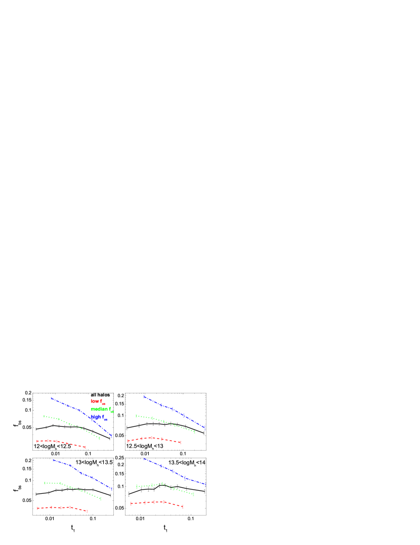
Figure 8: Here halos of a given mass are divided into three equal-size subsamples according to their $f_{\rm us}$. The colored lines show $f_{\rm us}$ as a function of $t_{1}$ for these three subsmaples, while the black line shows that for the total sample.

The measurement of $f_{\rm bs}$ from simulation can be affected by mass resolution, because some small subhalos are unresolved. Here we give a rough estimation of this effect. It is well known that the cumulative subhalo mass function is well-fit by a power-law $N(>M_{s})=A(M_{s}/M_{h})^{-1}$ down to $M_{s}\simeq 10^{-5}M_{h}$(e.g. Diemand et al. 2007), where $M_{s}$ is the subhalo mass and the amplitude $A$ depends on halo properties (e.g. Moore et al. 1999; Gao et al. 2004). Therefore $f_{\rm bs}(M_{sc}/M_{h})\simeq A\ln(M_{h}/M_{sc})=A\ln(N_{h}/10)$, where $N_{h}$ is the number of dark matter particles within the halo, and $M_{sc}=10M_{p}$ is the mass of the smallest subhalos identified. Clearly, the substructure mass fraction to be measured is sensitive to the particle number contained in the host. To reduce this effect, we divide halos into several narrow mass bins with size of 0.5 dex. In each mass bin, the variation of $f_{\rm bs}$ due to mass resolution is $\log(0.5\ln 10)\simeq 0.06$ dex, much less than the intrinsic scatter (more than 1 dex, see figure 8 of Gao et al. 2004). On the other hand, in order to make sure that the measured $f_{\rm bs}$ is not dominated by statistical variation, $M_{sc}/M_{h}$ has to be sufficiently small. As adopting $M_{sc}/M_{h}\leq 0.3\%$, more than half of mass in subhalos of $M_{s}\geq 10^{-5}M_{h}$ can be identified and the statistical variation is thus small. This suggests that $f_{\rm bs}$ can be reliably determined for halos containing more than 3300 particles. The mass resolution does not have a significant effect on the parameter $f_{\rm us}$. If the unresolved subhalos are not bound to the main halo, they must be contained in the fuzz. Therefore the unresolved subhalos still contribute to $f_{\rm us}$ without being missed. The uncertainty in $f_{\rm us}$ is expected to be less than $1/N_{h}$. For $N_{h}>3300$, it is much smaller than the typical value of $f_{\rm us}$ (see the following).

2.4 Halo spin parameters

The importance of the rotational motion relative to the internal random motion within a halo is usually described by a dimensionless spin parameter (Peebles 1969), defined as,

$$\lambda=\frac{J|E|^{1/2}}{GM_{h}^{5/2}}$$ (2)

where $G$ is Newton’s gravitational constant, $E$ is the total energy and $J$ the magnitude of angular momentum of the halo. We calculate the total energy using the method described in Bett et al. (2007). If a FOF halo contains more than 4000 particles, the total energy is computed using a random set of 4000 particles; otherwise all particles are used. We have measured the angular momentum, $J$, relative to the mass center whose velocity is defined by an average over all particles contained in the halo. We use $\hat{j}$, the direction of halo angular momentum, to denote the rotational axis of the halo.

2.5 Halo shapes and orientations

We use the inertia momentum tensor, ${\cal I}$, of a halo to characterize its shape and orientation (Jing et al. 1995). The components of ${\cal I}$ are estimated using

$$I_{jk}=M_{p}\sum^{N}_{n=1}x_{n,j}x_{n,k},$$ (3)

where $x_{n,j}$ ($j=1,2$ or 3) are the components of the position vector of the $n$th particle relative to the center of mass of the halo. The square root of the eigenvalues of this inertia momentum tensor are often used to represent the principal axes, $I_{1}$, $I_{2}$ and $I_{3}$ ($I_{1}\geq I_{2}\geq I_{3}$). In this paper, we use the axis ratios, e.g. $I_{3}/I_{1}$, to characterize the shape of a halo, and the corresponding unit vectors, $\hat{I}_{1}$, $\hat{I}_{2}$ and $\hat{I}_{3}$ to denote the directions of the major, intermediate and minor axes, respectively.

The estimates of both the spin parameter and the axial ratio can be affected significantly by numerical resolutions. As shown in Bett et al. (2007), in order to estimate these two parameters reliably, one needs more than 300 particles to sample a halo. To achieve such mass resolution and at the same time to obtain sufficient number of halos to perform the statistical analysis, we use the simulation sets L150 to study halos with masses $12<\log(M_{h}/\,h^{-1}{\rm M_{\odot}})<13$ (so that each halo contains more than 4270 particles) and use L300 to study halos with $\log(M_{h}/\,h^{-1}{\rm M_{\odot}})>13$ (more than 5300 particles per halo). Since the environmental effects on halo assembly time is strong only for low-mass halos (see below), we will include halos with $10.7<\log(M_{h}/\,h^{-1}{\rm M_{\odot}})<11$ (more than 210 particles per halo) in the L150 simulations when assembly time is considered. In most case, we do not consider halos of with $\log(M_{h}/\,h^{-1}{\rm M_{\odot}})>14.5$, because the total number of halos in this mass range is too small to give statistically reliable results.

3 Correlations among halo properties

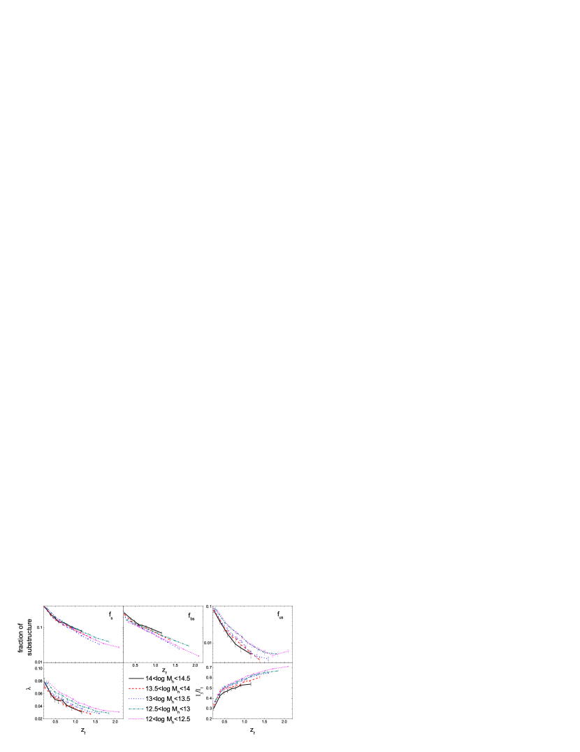
Figure 1: Median values of the fraction of total substructure, $f_{\rm s}$, fraction of bound substructure, $f_{\rm bs}$, fraction of unbound substructure, $f_{\rm us}$, spin parameter, $\lambda$, and short-to-long axis ratio, $I_{3}/I_{1}$, as functions of halo assembly time, $z_{\rm f}$, for halos of various masses. The halo mass range for each case is shown in the lower-middle panel.

We first examine how halo properties, such as $f_{\rm s}$, $f_{\rm us}$, $f_{\rm bs}$, $\lambda$, and $I_{3}/I_{1}$, are correlated with halo assembly time (specified by $z_{\rm f}$). The median values of these parameters as functions of $z_{\rm f}$ for various narrow mass bins are plotted in Fig. 1. The errors, $e_{y}$, on the median of a parameter, $y$, shown in the figures are computed using

$$e_{y}=\frac{y_{84}-y_{16}}{\sqrt{N_{halo}}}\,,$$ (4)

where $N_{halo}$ is the number of halos in each $z_{\rm f}$ bin (note that bin sizes are chosen so that each bin contains an equal number of halos), $y_{84}$ and $y_{16}$ denote the 84th and 16th percentiles of the distribution of $y$, corresponding to a $1\sigma$ spread if the underlying distribution were Gaussian.

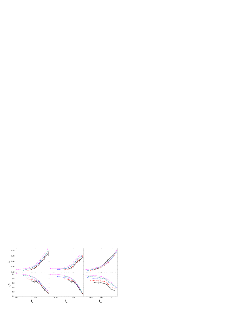
Figure 2: Median values of $\lambda$ and $I_{3}/I_{1}$ as functions of $f_{\rm s}$, $f_{\rm bs}$ and $f_{\rm us}$ for halos in the same five mass bins as shown in Fig. 1

All halo properties considered here show significant correlation with the assembly time. On average, young halos (those with lower $z_{\rm f}$) contain more substructures, spin more rapidly and are less spherical, than old halos of the same mass. These results are consistent with those found before (e.g. Jing & Suto 2002; Gao et al. 2004; Allgood et al. 2006; Hahn et al. 2007a). Many authors have interpreted these correlations as due to the fact that newly accreted halos may survive in their host halos (Gao et a. 2004), so as to significantly enhance the spin of the hosts (e.g. Vitvitska et al. 2002; Hetznecker & Burkert 2006), and to make the hosts more elongated (e.g. Hopkins et al. 2005). Such interpretation is supported by the fact that halo spin and shape have stronger correlation with the substructure fraction than with the assembly time (see Fig. 2 below). Furthermore, we find that the $z_{f}$-dependence of the short-to-intermediate axial ratio, $I_{3}/I_{2}$, is much weaker than the other two ratios, indicating that new material tends to be accreted along the major axes of halos (Wang et al. 2005).

However, other processes may also be important, at least for some of these correlations. For instance, D’Onghia & Navarro (2007) found that the spins of halos that have ceased growing can still drop gradually, presumably due to mass redistribution such as the ejection of high-angular momentum material from the halo during the subsequent virialization process. Indeed, as shown in Wang et al. (2009b), there is clear evidence that old halos tend to eject more subhalos than young ones of the same mass. A correlation between halo spin and assembly time can thus be produced via this process. Clear, more detailed analysis are needed to quantify the role of such mechanism.

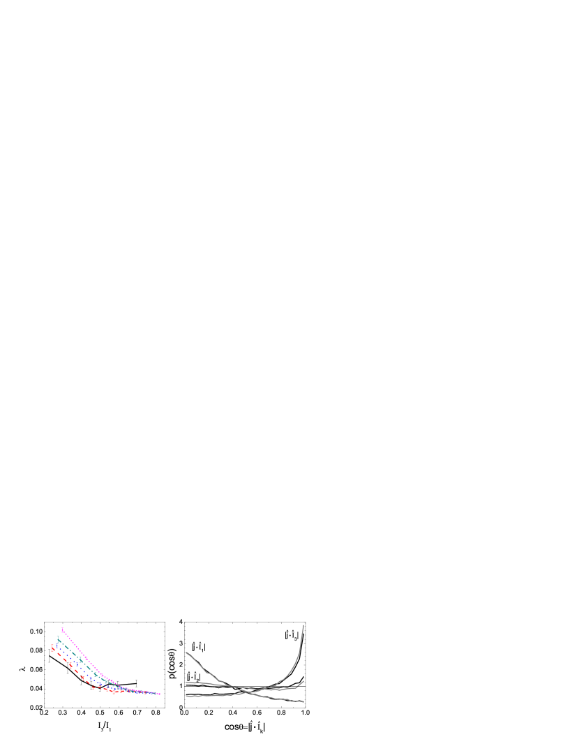
Figure 3: The left panel shows the median $\lambda$ as a function of short-to-long axis ratio $I_{3}/I_{1}$ for halos for halos in the same five mass bins as shown in Fig. 1. The right panel shows the probability distribution of the cosine of the angle between the spin vector, $\hat{j}$, and the three principal axes $\hat{I}_{k}$. The black and grey lines are for halos with $13<log(M_{h}/\,h^{-1}{\rm M_{\odot}})<14.5$ and $12<log(M_{h}/\,h^{-1}{\rm M_{\odot}})<13$, respectively. The horizontal line indicates a random distribution.

Fig. 2 shows how halo spin and axis ratio are correlated with the substructure fractions. Both $\lambda$ and $I_{3}/I_{1}$ depend strongly on unbound and bound fractions. This is consistent with Maccio’ et al. (2007; see also Shaw et al. 2006) who found that unrelaxed halos tend to spin more rapidly and to be more prolate. As one can see from the left panel of Fig.3, which shows the correlation between halo spin and halo axis ratio, less spherical halos, especially the ones with low masses, tend to have higher $\lambda$. In the right panel of the figure, we show the probability distribution function of the cosine of the angle between the spin vector, $\hat{j}$, and the three principle axes of the halo, $\hat{I}_{1}$, $\hat{I}_{2}$ and $\hat{I}_{3}$. Since we do not find any evidence for such alignment to depend on halo mass, results are shown only for two mass bins. As one can see, the spin axis has the tendency to be parallel to the minor axis and perpendicular to the major axes (see also Warren et al. 1992; Shaw et al. 2006; Bett et al. 2007; Zhang et al. 2009).

Inspecting these correlations in detail, we can find several interesting trends. First, the dependence of halo spin on $f_{\rm us}$ is stronger than on any other halo properties, such as $z_{\rm f}$ and $f_{\rm bs}$. In contrast, the halo axial ratio shows stronger correlation with $z_{\rm f}$ and $f_{\rm bs}$ than with $f_{\rm us}$. Second, the relationships among $f_{\rm bs}$, $z_{\rm f}$ and $I_{3}/I_{1}$ (see the upper-middle and lower-right panels of Fig. 1, and the lower-middle panel of Fig. 2) and between $f_{\rm us}$ and $\lambda$ (see the upper-right panel of Fig. 2) have only weak dependencies on halo mass, while the relationships between these two sets of halo properties depend significantly on halo mass. These tendencies suggest that $f_{\rm bs}$, $z_{\rm f}$ and $I_{3}/I_{1}$ may have similar origin, and so do $f_{\rm us}$ and $\lambda$. In Section 5 we will investigate how these halo properties depend on halo environment, and we will see that $f_{\rm bs}$, $z_{\rm f}$ and $I_{3}/I_{1}$ exhibit similar environmental dependence, while $f_{\rm us}$ and $\lambda$ exhibit common environmental dependence different from that of the other three halo properties.

4 Large-scale tidal field traced by halos

In the literature a number of parameters have been used to quantify the large-scale environments. These include the local mass overdensity around halos, the halo bias parameter, the morphology of large scale structure, and the tidal field produced by large-scale mass distribution. In this paper we use the ‘halo tidal field’, obtained from the distribution of dark matter halos above a certain mass threshold $\,{\rm{M_{th}}}$, as our primary environmental parameters. As shown in Yang et al. (2005; 2007), galaxy groups/clusters properly selected from large redshift surveys of galaxies can be used to represent the dark halo population, especially massive ones with masses $\lower 2.15277pt\hbox{$\;\buildrel>\over{\sim}\;$}10^{12}\,h^{-1}{\rm M_{\odot}}$. Thus, the ‘halo tidal field’, can in principle be estimated from observation. In what follows we describe how the halo tidal field is defined and estimated. In Appendix B we examine how halo tidal field is correlated with the other environmental indicators mentioned above.

The normalized halo tidal force on the surface of a given halo, ‘h’, in a direction $\vec{t}$ is defined as

$$F_{t}(\vec{t})=\frac{\sum_{i=1}^{N}\frac{GM_{i}}{r_{i}^{3}}R_{h}(1/2+3/2\cos(2\theta_{i}))}{GM_{h}/R_{h}^{2}}=\sum_{i=1}^{N}\frac{R_{i}^{3}}{2r_{i}^{3}}(1+3\cos{2\theta_{i}})\,,$$ (5)

where $M_{h}$ and $R_{h}$ are the mass and radius of the halo in question, $M_{i}$ and $R_{i}$ are the masses and radii of other halos producing the tidal force, $r_{i}$ is the distance from halo ‘$h$’ to halo ‘$i$’, and $\theta_{i}$ is the angle between $\vec{t}$ and $\vec{r}_{i}$. The second equation follows from the fact that the mean density within the virial radius at a given redshift is the same for all halos, so that $M_{h}\propto R_{h}^{3}$ and $M_{i}\propto R_{i}^{3}$. Thus, the tidal force on a halo is calculated by summing up the tidal forces of all other halos of mass above $\,{\rm{M_{th}}}$, and is normalized by the self-gravity of the halo in question, so that one can compare the environmental effects for halos of different masses. We define the halo tidal force on the halo surface so that we can easily quantify/distinguish between the self-gravity or tidal force dominated impact on the particles that are to be accreted to or to be ejected from the halos. In the following, we adopt a threshold mass $\,{\rm{M_{th}}}=10^{12}\,h^{-1}{\rm M_{\odot}}$, which is the low mass limit of groups selected from current galaxy redshift surveys (e.g. Yang et al. 2007). And as we have tested, using somewhat larger or smaller $\,{\rm{M_{th}}}$ does not change any of our results significantly.

We first define two tidal directions, $\vec{t}_{1}$ and $\vec{t}_{3}$, so that the tidal force has the largest value along $\vec{t}_{1}$ and the lowest value along $\vec{t}_{3}$. According to the analysis presented in the Appendix, vectors $\vec{t}_{1}$ and $\vec{t}_{3}$ are the eigenvectors of the halo tidal tensor, are perpendicular to each other, and represent the major and minor axes of the halo tidal field. The third tidal direction, $\vec{t}_{2}$, is defined as a vector perpendicular to both $\vec{t}_{1}$ and $\vec{t}_{3}$. We use $t_{1}$, $t_{2}$ and $t_{3}$ to denote the tidal forces along $\vec{t}_{1}$, $\vec{t}_{2}$ and $\vec{t}_{3}$, respectively. Different from the tidal field produced by large-scale mass distribution, halo tidal field satisfies $t_{1}+t_{2}+t_{3}=0$ (see Appendix A); thus only two parameters are needed to characterize the halo tidal field. We adopt $t_{1}$ to represent the magnitude and a parameter,

$$t_{s}\equiv\frac{t_{1}-t_{2}}{t_{1}+t_{2}}\,,$$ (6)

to characterize the ‘shape’ of the tidal field. Clearly, $t_{s}$ describes the anisotropy in the distribution of neighboring halos. If $t_{s}>1$, then both $t_{2}$ and $t_{3}$ must be negative while $t_{1}>0$. Thus the tidal field stretches the material along $\vec{t}_{1}$, but compresses it in the other two directions. This also means that halos dominating the tidal field must be distributed preferentially along $\vec{t}_{1}$ in a filamentary structure. In the extreme case of $t_{s}=3$, the tidal field is dominated by just one halo. If $t_{s}<1$, then $t_{2}>0$ so that the tidal field compresses halo material only along $\vec{t}_{3}$, while stretches it along both $\vec{t}_{1}$ and $\vec{t}_{2}$. Such a tidal field can be produced by more than one halos distributed preferentially in the $\vec{t}_{1}$-$\vec{t}_{2}$ plane.

5 Correlations between halo properties and environment

In this section, we explore the correlations between halo properties and their environments. The goal is to find out which environmental effects have the strongest impact on halo properties, and whether there is any connection between different environmental effects. Since halo mass may be correlated with both environment and other halo properties, it is sometimes necessary to divide halos into narrow mass bins in order to identify possible causal connections between halo properties and environment. In such cases we divide halos into mass bins with a size of 0.5 dex or smaller.

5.1 Assembly time

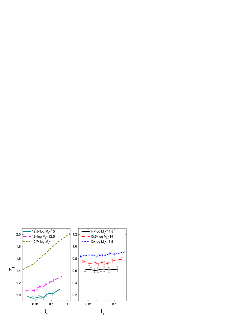
Figure 4: The median assembly time, $z_{\rm f}$, as a function of the tidal field $t_{1}$ for halos of different masses (in units of $\,h^{-1}{\rm M_{\odot}}$).

It has been found that the clustering of low-mass halos depends on their assembly times (e.g. Gao et al. 2005). Wang et al. (2007a) found that old, low-mass halos have a tendency to reside in the vicinity of massive systems, and suggested that the tidal truncation of accretion may be responsible for the assembly bias (see also Keselman & Nusser 2007; Desjacques 2008). In Fig. 4, we show the relation between halo assembly time, $z_{\rm f}$, and the halo tidal field represented by $t_{1}$. As one can see, the median assembly time increases with $t_{1}$ for low-mass halos, and the dependence becomes weaker with the increase of halo mass.

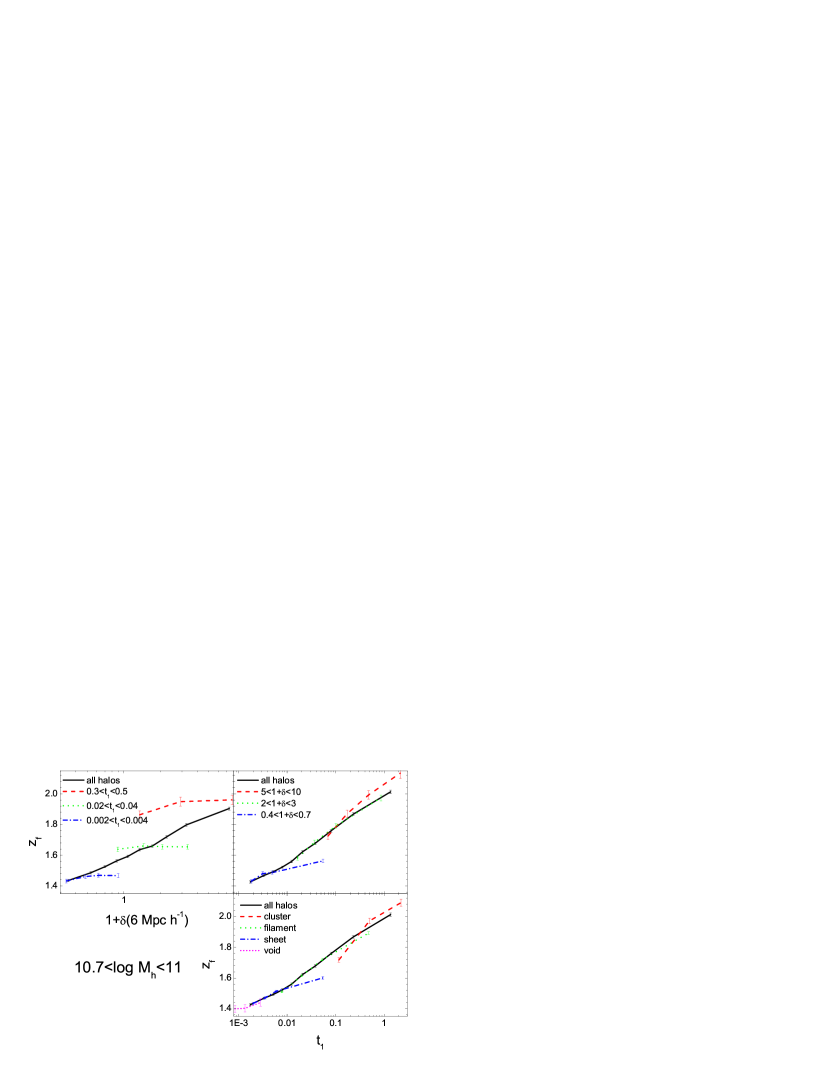
Figure 5: The black solid line in each panel shows the median $z_{\rm f}$ as a function of local overdensity (upper left panel) and $t_{1}$ (the two right panels) for halos of $10.7<log(M_{h}/\,h^{-1}{\rm M_{\odot}})<11$. The colored lines show the results at fixed $t_{1}$ (upper left panel), fixed local overdensity (upper right panel), and for given types of large-scale structure (lower right panel), as indicated in each panel.

Since $t_{1}$ is correlated with the large-scale density field and the morphology of large scale structure (see Appendix B), the dependence of assembly time on tidal field might originate from the correlation between assembly time with these other environment quantities. Clearly, further analysis is required in order to examine which quantity plays the more primary role in affecting halo assembly. Since strong environmental dependence of $z_{\rm f}$ exists only for low-mass halos, we concentrate on halos with $10.7<\log(M_{h}/\,h^{-1}{\rm M_{\odot}})<11$. The upper-left panel of Fig. 5 shows the median assembly time versus $1+\delta(6\,h^{-1}{\rm{Mpc}})$, where $\delta(6\,h^{-1}{\rm{Mpc}})$ is the overdensity of dark matter within a sphere of radius 6 $\,h^{-1}{\rm{Mpc}}$ around each dark matter halo (defined in Appendix B). It is evident that halos in higher density regions have earlier assembly time. For comparison, we sub-divide the halos into three narrow $t_{1}$ bins, and show the corresponding $z_{\rm f}$ - $1+\delta(6\,h^{-1}{\rm{Mpc}})$ relation in the same panel of Fig. 5. As one can see, at a fixed value of $t_{1}$ the correlation between $z_{\rm f}$ and $1+\delta(6\,h^{-1}{\rm{Mpc}})$ is almost absent. In contrast, for fixed local overdensity, the dependence of $z_{\rm f}$ on $t_{1}$ is almost as strong as the overall trend (the upper-right panel of Fig. 5). In particular, the correlation is significant even in underdense regions (see the blue-dash dot line in the upper-right panel of Fig. 5). As a further test we show, in the bottom panel of Fig. 5, the correlation between $z_{\rm f}$ and $t_{1}$ separately for halos in clusters, filaments, sheets and voids, as defined in Appendix B. Clearly, the dependence of $z_{\rm f}$ on $t_{1}$ is not affected significantly by the morphology of the environment. We have made calculations using overdensities in spheres with radii other than $6\,h^{-1}{\rm{Mpc}}$ and found that our results are robust against such change. The results are similar for halos with $\log(M_{h}/\,h^{-1}{\rm M_{\odot}})<11.7$. However, for halos with $\log(M_{h}/\,h^{-1}{\rm M_{\odot}})>11.7$, the environmental effect is too weak, compared to the correlations among different environmental indicators, to break the degeneracy.

All these results unequivocally demonstrate that the amplitude of the halo tidal field, represented by $t_{1}$, is the primary environmental factor that has the most important impact on halo assembly. This is consistent with suggestion made by Wang et al. (2007a) that the large-scale tidal field may accelerate mass around halos, especially low-mass ones, and truncate their mass accretion. The dependence of halo assembly time on local overdensity and on the morphology of the environment is the secondary effect induced by the tidal force. As shown in Fig. 5, the tidal effect exists even for $t_{1}<0.005$, where the self-gravity is much larger than the tidal force. Thus, it is tidal truncation rather than tidal stripping that is responsible for the halo assembly bias.

5.2 Mass fraction in substructures

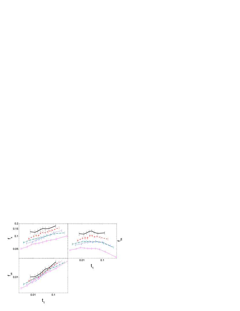
Figure 6: The median values of halo properties $f_{\rm s}$, $f_{\rm us}$ and $f_{\rm bs}$ as functions of $t_{1}$. Results are shown for halos in the same five mass bins as in Fig. 1.

Fig. 6 shows the correlations between the tidal parameter, $t_{1}$, and the mass fraction in total substructure, $f_{\rm s}$, in the bound substructure, $f_{\rm bs}$, and in the unbound substructure, $f_{\rm us}$. Here SUBFIND (Springel et al. 2001) was used to identify subhalos; bound substructures are defined to be subhalos with negative total energy relative to the main halo, while unbound substructures are unbound subhalos plus fuzz. Clearly, the amounts of total substructures tend to be larger in high-$t_{1}$ environments. Thus, halo clustering strength is expected to depend on the substructure fraction (e.g. Gao & White 2007; Ishiyama, Fukushige, & Makino 2008). However, the environmental dependence of the substructure fraction becomes very different after the removal of the unbound component; the dependence of bound component on $t_{1}$ is totally absent for massive halos, and there is a weak, but significant, trend that $f_{\rm bs}$ actually declines with increasing $t_{1}$ for low-mass halos. Such halo mass dependence of the $f_{\rm bs}$-$t_{1}$ relation is very similar to the halo mass dependence of the $z_{f}$-$t_{1}$ relation. Unbound substructure fraction also increases with increasing $t_{1}$. In particular, this correlation is much stronger and is almost halo mass independent. These results suggest that the $t_{1}$-$f_{\rm s}$ correlation is dominated by the environmental dependence of $f_{\rm us}$. Since $f_{s}$ is a measure of the mass a halo assembles after the formation of its main halo and $f_{\rm us}$ is the unbound fraction, the results reflect the fact that regions of stronger tidal field, which are also of higher densities, provide more material for halo to accrete, but the tidal effect in these regions are also stronger so that $f_{\rm us}$ increases rapidly with $t_{1}$.

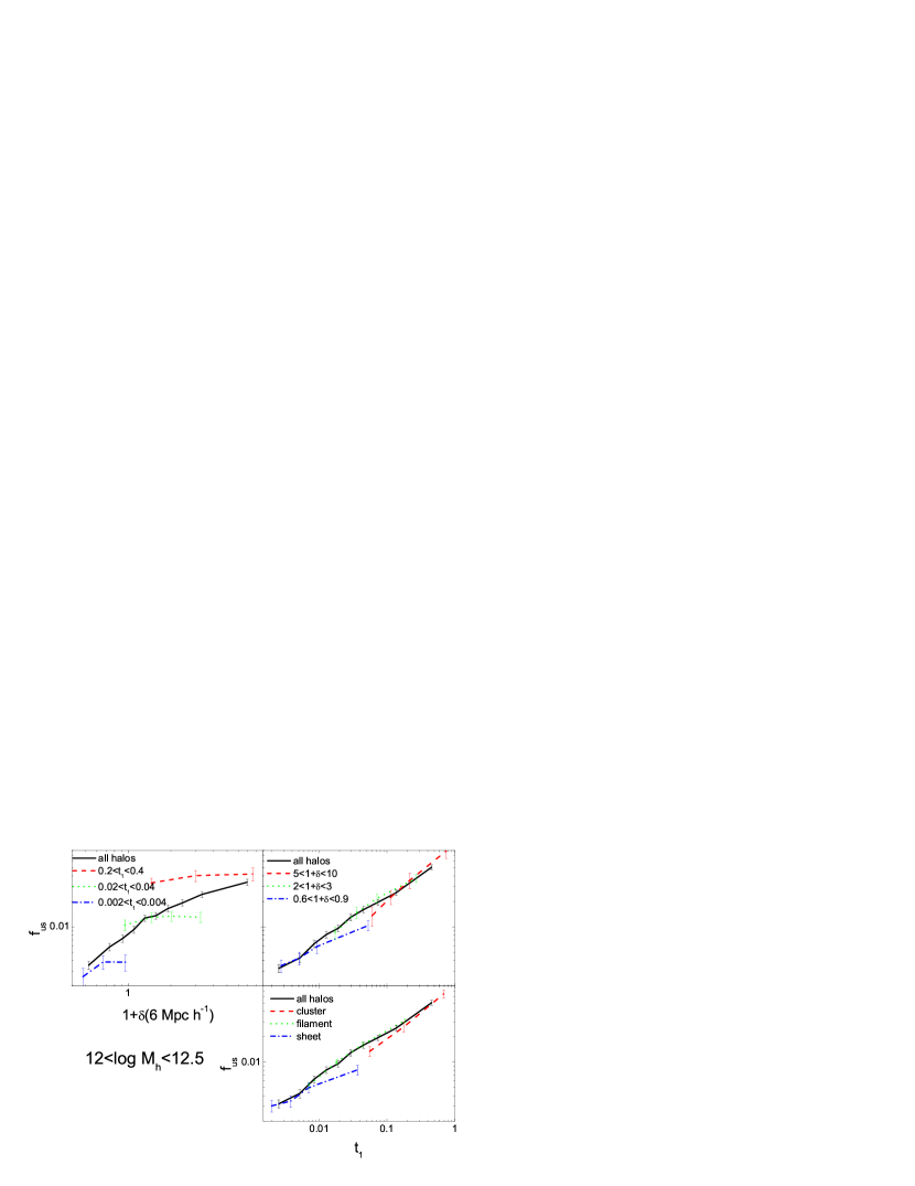
Figure 7: The black solid line in each panel shows the median $f_{\rm us}$ as a function of local overdensity (upper left panel) and $t_{1}$ (the two right panels) for halos of $12<log(M_{h}/\,h^{-1}{\rm M_{\odot}})<12.5$. The colored lines show the results at fixed $t_{1}$ (upper left panel), fixed local overdensity (upper right panel), and for given types of large-scale structure (lower right panel), as indicated in each panel.

Similar results are obtained when local overdensity or halo bias are used instead of the tidal field as the environmental indicator. In order to examine which environmental property is more responsible to the strong dependence of $f_{\rm us}$ on environment, we show $f_{\rm us}$ as a function of $1+\delta(6\,h^{-1}{\rm{Mpc}})$ in the upper-left panel of Fig. 7, together with the results for halos residing in environments with the same $t_{1}$. In comparison, we also show $f_{\rm us}$ as a function of $t_{1}$ at fixed $\delta(6\,h^{-1}{\rm{Mpc}})$ and for given types of large-scale structure. The results clearly demonstrate that it is the tidal field that plays the dominating role in affecting the unbound fraction. Note that the figure only presents the results for halos with $12<\log(M_{h}/\,h^{-1}{\rm M_{\odot}})<12.5$ and using overdensity on a scale of $6\,h^{-1}{\rm{Mpc}}$, but our tests using overdensity on different scales and halos with $12.5<\log(M_{h}/\,h^{-1}{\rm M_{\odot}})<13$ and $13<\log(M_{h}/\,h^{-1}{\rm M_{\odot}})<13.5$ lead to the same conclusion.

According to our definition, only when $t_{1}\mathrel{\raise 1.16pt\hbox{$>$}\kern-7.0pt\lower 3.06pt\hbox{{$\scriptstyle\sim$}}}1$ can the tidal force overcome halo’s self-gravity to cause significant stripping. However, the dependence on $t_{1}$ extends all the way to $t_{1}<0.005$, and is significant even in underdense regions and in sheet-like structure (Fig. 7). This suggests that this effect cannot be produced via tidal stripping. Alternatively, large-scale tidal field may accelerate the material around a halo, causing them to move quickly relative to the halo (e.g. Wang et al. 2007a; Hahn et al. 2009; Fakhouri & Ma 2009). Some of these energetic particles and satellites may be falling into dark matter halos but may not be bound to them. One support for this hypothesis is the existence of a population of ejected halos, which were once contained in massive halos but eventually would leave their hosts (e.g. Wang et al. 2009b).

As mentioned above, there are two environmental effects that can affect a halo’s assembly. On the one hand, the amount of the material that fuels the accretion increases with local density. Halos in high-density regions are thus expected to have higher $f_{\rm s}$ and lower $z_{\rm f}$. On the other hand, the tidal field in a high-density region is on average stronger so that a larger fraction of the accreted material may become unbound to the halo, in particular for low-mass halos where tidal force is more important relative to halo self-gravity. This would make halos in high-density regions more difficult to grow. The growth of a halo is therefore the result of the competition between these two processes, and they affect halo properties in different ways, depending on the halo mass. For low-mass halos where tidal suppression of growth is more important, halos in high tidal force/density regions are expected to have lower $f_{\rm bs}$ and to form earlier (with higher $z_{\rm f}$). For massive halos, on the other hand, the two effects may play comparable roles, so that the environmental dependence of bound substructure and of halo assembly time is reduced. The two processes acting together produce a much stronger environmental dependence for $f_{\rm us}$ than for $f_{\rm s}$ regardless of halo masses.

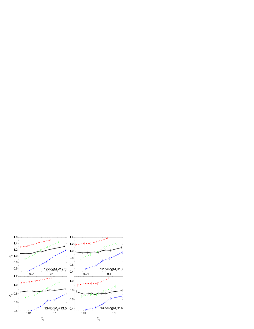
Figure 9: The same as Fig.8 but for the halo assembly time $z_{\rm f}$ as a function of $t_{1}$.

The second process results in a change of the ratio between bound and unbound components with tidal force for both low-mass and massive halos. To verify this, we make further analysis by dividing halos into three equally-sized subsamples according to their $f_{\rm us}$ and examining the $t_{1}$ - $f_{\rm bs}$ correlation separately for these subsamples. The results for these four mass bins are shown in Fig. 8. Significant anti-correlation between the tidal force and bound substructure fraction is indeed found for all these subsamples, even though it is absent in the whole sample of massive halos. Fig.9 show the correlation between $t_{1}$ and $z_{\rm f}$ for these subsamples. Clearly, halos form earlier in high tidal-force environment for all these subsamples, even though this effect does not show up in the total sample of massive halos. The amount of material with energy sufficiently low to be accreted is smaller in an environment of stronger tidal field, so that the amount of bound substructure and halo growth are both suppressed. Our finding naturally explains the apparent conflict in the bias-$z_{\rm f}$ relation, the bias - $f_{\rm s}$ relation and the $z_{\rm f}$ - $f_{\rm s}$ relation (see Gao & White 2007). Note that the absence of strong $t_{1}$-$f_{\rm bs}$ and $t_{1}$-$z_{\rm f}$ correlations for the lowest $f_{\rm us}$ subsample is due to the use of non-zero $f_{\rm us}$-bin size. Our test showed that the correlations indeed appear when this subsmaple is divided further into narrower $f_{\rm us}$ bins.

5.3 Halo shape and orientation

Table 1: The mean cosine of the angle between the principal axes of a halo and its orientation

$\log M_{h}(\,h^{-1}{\rm M_{\odot}})$	$<|\hat{I}_{1}\cdot\vec{t}_{1}|>$	$<|\hat{I}_{2}\cdot\vec{t}_{2}|>$	$<|\hat{I}_{3}\cdot\vec{t}_{3}|>$
$[14.5,15]$	0.75$\pm$0.02	0.60$\pm$0.02	0.74$\pm$0.02
$[14,14.5]$	0.732$\pm$0.006	0.560$\pm$0.007	0.674$\pm$0.007
$[13.5,14]$	0.698$\pm$0.003	0.547$\pm$0.004	0.642$\pm$0.004
$[13,13.5]$	0.647$\pm$0.002	0.526$\pm$0.002	0.601$\pm$0.002
$[12.5,13]$	0.600$\pm$0.003	0.515$\pm$0.003	0.583$\pm$0.003
$[12,12.5]$	0.567$\pm$0.002	0.506$\pm$0.002	0.567$\pm$0.002

Hahn et al. (2007b) found halo major axes are strongly aligned with that of tidal field. We confirm their results using halo tidal field. The mean values of $|\hat{I}_{1}\cdot\vec{t}_{1}|$ are listed in Table 1. For comparison, we also list the corresponding results for the intermediate and minor axes. Clearly, there is a strong alignment between $\hat{I}_{1}$ and $\vec{t}_{1}$, and between $\hat{I}_{3}$ and $\vec{t}_{3}$, but the alignment between $\hat{I}_{2}$ and $\vec{t}_{2}$ is much weaker. The alignments are also stronger for more massive halos.

Since substructures tends to fall into the host halos along the filament (e.g. Wang, et al. 2005; Altay, Colberg & Croft 2006), one might think that the alignments are dominated by the presence of substructure. In order to test this, we make calculations using only particles contained by the main halos to calculate the tensor of inertia. There is little change in the alignments, demonstrating that the main halos are also aligned with the tidal field.

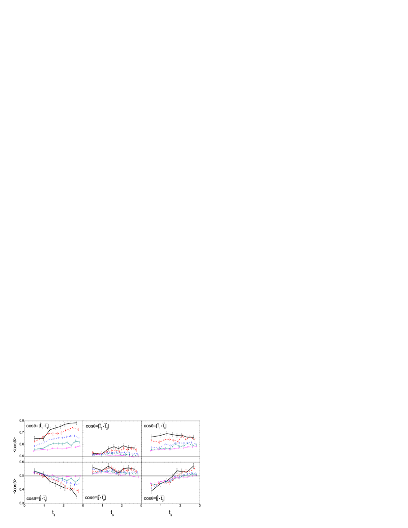
Figure 10: The upper three panels show the mean of $|\hat{I}_{k}\cdot\vec{t}_{k}|$ as a function of the shape of tidal field, $t_{s}$. The lower panels show the mean of $|\hat{j}\cdot\vec{t}_{k}|$ as a function of $t_{s}$. Results are shown for halos in the same five mass bins as in Fig. 1. The horizontal lines indicate random distribution.

In the upper panels of Fig. 10, we show the average of $|\hat{I}_{k}\cdot\vec{t}_{k}|(k=1,2,3)$ as a function of $t_{s}$. The alignment of major axes shows significant dependence on $t_{s}$; halos in regions with higher values of $t_{s}$ (i.e. where the tidal field is more anisotropic) tend to be more strongly aligned with the tidal field. This trend is either weak or absent for the intermediate and minor axes.

These alignments may be the primary reasons for some of the alignments observed in simulations and observations, including the alignment between the orientations of neighboring galaxy clusters (Binggeli 1982; Chambers et al. 2002), the alignment between the orientation of the brightest cluster/group galaxy and the distribution of its satellites (Carter & Metcalfe 1980; Wang et al. 2008b; Faltenbacher et al. 2007; Kang et al. 2007), the alignment between the galaxy/galaxies cluster orientations and large-scale structure (Hirata et al. 2007; Faltenbacher et al. 2009; Wang et al. 2009c; Okumura & Jing 2009; Okumura, Jing & Li 2009), and furthermore the dependence of the alignments on halo mass (e.g. Jing 2002; Yang et al. 2006b). One possibility is that the accretion onto a dark matter halo occurs through a dominating filament, so that the halo is elongated along the filament (e.g. Van Haarlem & Van deWeygaert 1993; Altay et al. 2006). Since the major axis of the tidal field is expected to trace well the direction of the local filamentary structure (Hahn et al. 2007b; Zhang et al. 2009), a strong alignment between $\hat{I}_{1}$ and $\vec{t}_{1}$ can be produced. However, such a mechanism is difficult to explain the $\hat{I}_{3}$ - $\vec{t}_{3}$ alignment, which is as strong as the $\hat{I}_{1}$ - $\vec{t}_{1}$ alignment. Alternatively and perhaps more likely, the collapse of a density perturbation to form a halo may be affected by the tidal field, as in the ellipsoidal collapse model (see Sheth, Mo & Tormen 2001; Shen et al. 2006), and the halo orientation is a result of the corresponding triaxial collapse.

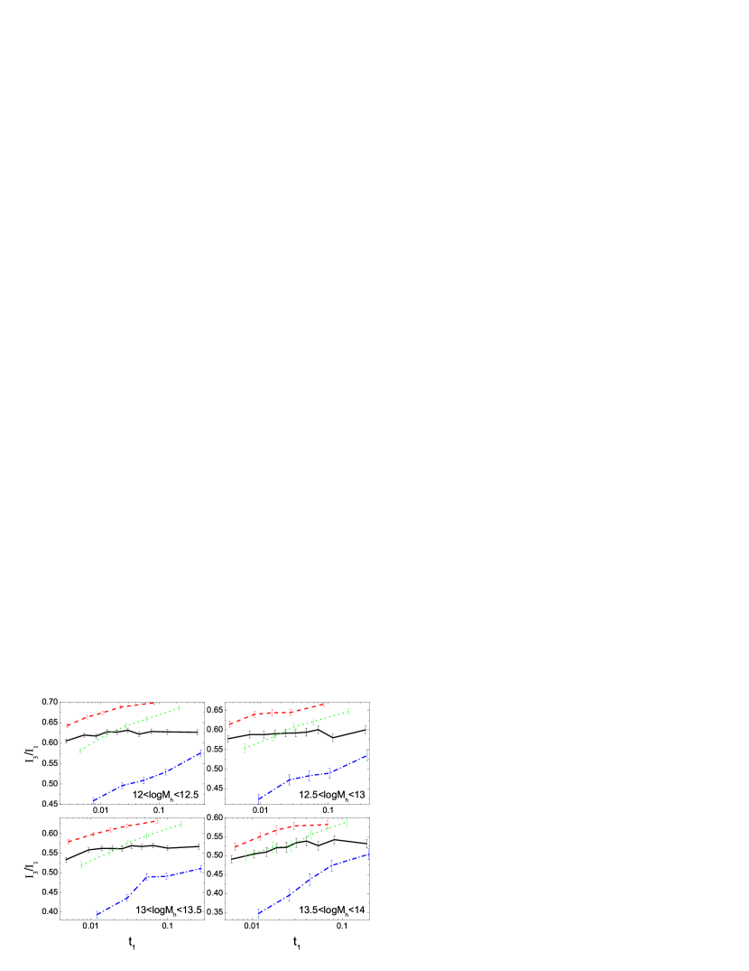
Figure 11: Here halos of a given mass are divided into three equal-size subsamples according to their $f_{\rm us}$. The colored lines show $I_{3}/I_{1}$ as a function of $t_{1}$ for these three subsmaples, while the black line shows that for the total sample.

In addition to the alignment of halos with tidal field, we also study how the axis ratio of a halo, for example $I_{3}/I_{1}$, is correlated with the tidal field. In Fig. 11, we show the median value of $I_{3}/I_{1}$ as a function of $t_{1}$ ( black solid lines) for halos of four mass bins. Only most massive sample shows some weak trend that halos in stronger tidal field tend to be more spherical. Moreover, the axis ratio is independent of $t_{s}$ for halos of all masses. Bett et al. (2007) investigated the environmental dependence of halo shape and found that spherical halos are more strongly clustered than the more aspherical ones. This is different from our results. To compare with their results more directly, we compute the halo bias as a function of $I_{3}/I_{1}$ (see Appendix B for how halo bias is defined and computed). Similar to the $t_{1}$ - $I_{3}/I_{1}$ correlation, no significant trend as seen by Bett et al. is found. The difference may be due to the fact that Bett et al. only considered halos in quasi-equilibrium state. Since the virialization of a halo is related to the substructure fraction (Shaw et al. 2006), we divide the halos into three equally-sized subsamples according to $f_{\rm us}$ and re-examine the environmental dependence separately for these subsets of halos. The results are shown in Fig.11 to compare with the total sample. In each subsmaple, halos are more spherical in high tidal force region. As shown in Fig.2, the axis ratio depends strongly on the bound substructure fraction, $f_{\rm bs}$. As $t_{1}$ increases, $f_{\rm bs}$ decreases and the halo becomes more spherical. This effect is absent for the full sample because higher $f_{\rm us}$ halos are more elongated (Fig. 2) and have a stronger tendency to reside in higher tidal force region (Fig. 6), compensating the trend.

5.4 Halo spin

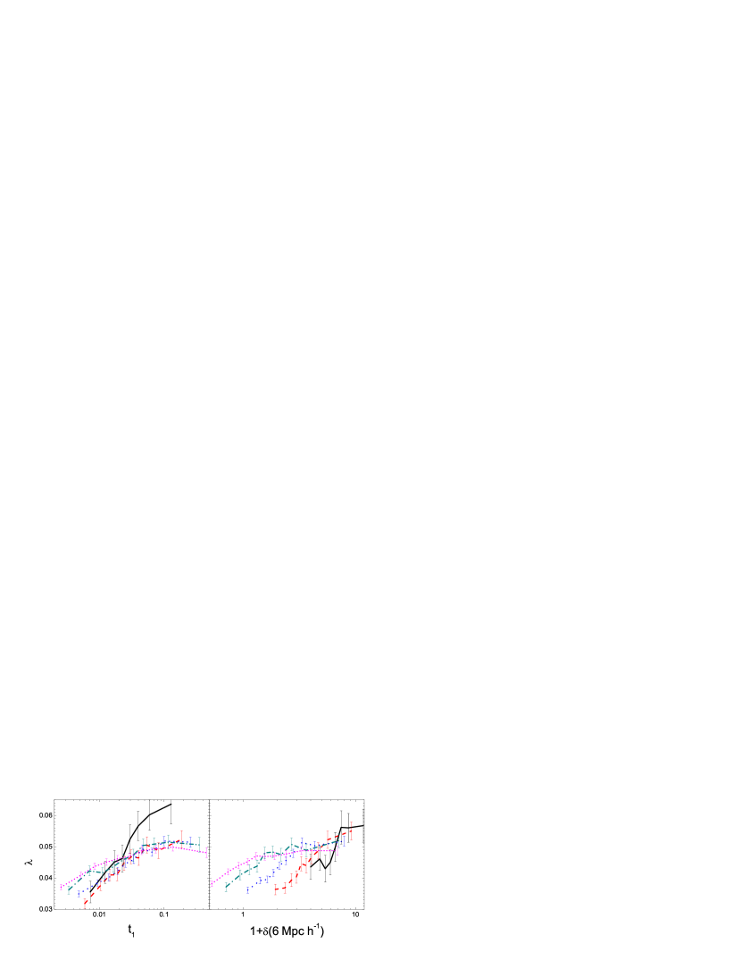
Figure 12: The median of the spin parameter, $\lambda$, as a function of tidal force, $t_{1}$ (left panel) and local overdensity, $\delta(6\,h^{-1}{\rm{Mpc}})$ (right panel). Results are shown for halos in the same five mass bins as in Fig. 1.

According to the tidal torque theory, the angular momenta of dark matter halos is generated by large-scale tidal field (e.g. Peebles 1969; Doroshkevich 1970). In the left panel of Fig. 12 we show the dependence of $\lambda$ on $t_{1}$. Clearly halos tend to spin faster in stronger tidal field, and this trend is stronger for massive halos. However the dependence is rather weak. The value of $\lambda$ increases by a factor less than two as the value of $t_{1}$ increases by an order of magnitude, much weaker than the linear dependence expected from the tidal torque theory. Note that the dependence on $t_{s}$ is absent. It is known that halo clustering strength increases with halo spin (e.g. Bett et al. 2007). In order to make a direct comparison between these two environmental properties, we present $\lambda$ as a function of $\delta(6\,h^{-1}{\rm{Mpc}})$, instead of halo bias, versus $\lambda$ in the right panel of Fig. 12. The correlation strength is similar to that with tidal force.

Table 2: The mean cosine of the angle between spin axis of halo and the principle axes of halo tidal field

$\log M_{h}(\,h^{-1}{\rm M_{\odot}})$	$<|\hat{j}\cdot\vec{t}_{1}|>$	$<|\hat{j}\cdot\vec{t}_{2}|>$	$<|\hat{j}\cdot\vec{t}_{3}|>$
$[14.5,15]$	0.39$\pm$0.02	0.59$\pm$0.02	0.49$\pm$0.02
$[14,14.5]$	0.443$\pm$0.007	0.550$\pm$0.007	0.495$\pm$0.007
$[13.5,14]$	0.452$\pm$0.003	0.541$\pm$0.003	0.491$\pm$0.004
$[13,13.5]$	0.472$\pm$0.002	0.532$\pm$0.002	0.484$\pm$0.002
$[12.5,13]$	0.489$\pm$0.003	0.522$\pm$0.003	0.480$\pm$0.003
$[12,12.5]$	0.503$\pm$0.002	0.510$\pm$0.002	0.479$\pm$0.002

Since the frequency of halo merging increases with local density (e.g. Fakhouri & Ma 2009), the above correlations can also be interpreted via the merger scenario (Gardner 2001; Maller et al. 2002). To gain more insight, we examine the alignment between the halo angular momentum vector, $\hat{j}$, and the three principal axes of the tidal field, $\vec{t}_{k}$. The mean values of the dot product $|\hat{j}\cdot\vec{t}_{k}|$ for various halo masses are listed in Table 2. As one can see, halos obviously tend to spin around axes perpendicular to the major axes of the large-scale tidal field. The strength of the alignment decreases with decreasing halo mass and becomes absent for halos of $\log(M_{h}/\,h^{-1}{\rm M_{\odot}})\simeq 12$. Some recent studies have found a weak but significant alignment between the spin of low-mass halos ($\log(M_{h}/\,h^{-1}{\rm M_{\odot}})\simeq 11$) and the orientation of the large-scale mass distribution (Arag$\acute{{\rm o}}$n-Calvo et al. 2007; Paz et al. 2008; Zhang et al. 2009). Using the major axis of the halo tidal field to approximate the orientation of large scale mass distribution, we also detect such an alignment signal for halos in a similar mass range.

There is also a weak tendency for the spin axis to be perpendicular to the minor axis of tidal field, and the strength is weaker than that to the major axis of the tidal field in the mass ranges in consideration. In contrast, halo spin is aligned with the intermediate axis of tidal field (see Table 2). Such an alignment is a natural prediction of the tidal torque theory (e.g. Porciani et al. 2002; Lee & Erdogdu 2007), and so our result provides support to the tidal torque origin for the halo angular momentum. However, except for massive halos with $14.5<\log(M_{h}/\,h^{-1}{\rm M_{\odot}})<15$, the alignment strength we find (see Table 2) is much weaker than the value $0.59$ predicted by the tidal torque theory (Porciani et al. 2002), particularly for low-mass halos. Since the tidal torque theory is based on linear density field, the discrepancy may be due to non-linear evolution. Indeed, using N-body simulations, Porciani et al. (2002) did not find any alignment between halo spins and initial tidal field and concluded that non-linear effects completely erase the correlation. However, Porciani et al. (2002) focused on relatively low-mass halos, for which the alignment strength is weak according to our results. Significant correlation does exist for massive halos.

It has been suggested that the orientations of halo spin vectors are correlated with the morphology of the nearby large-scale mass distribution (e.g. Arag$\acute{{\rm o}}$n-Calvo et al. 2007; Hahn et al. 2007a; Zhang et al. 2009). For instance, the spin axes of halos in sheets tend to lie in the sheet, while halos in filaments have a tendency to spin around axes perpendicular to the filaments. Similar trends have also been claimed in observational data. Navarro, Abadi & Steinmetz (2004) found that the spin axes of nearby disk galaxies tend to lie on the supergalactic plane. Trujillo, Carretero & Patiri (2006) analyzed a large sample of spiral galaxies and found that galaxies that are located on the surfaces of cosmic voids have spin axes tending to be parallel to the surfaces.

As discussed above, the $t_{s}$ parameter defined in our analysis can be used to quantify the morphology of nearby mass/halo distribution. In the lower three panels of Fig. 10 we show the mean value of $|\hat{j}\cdot\vec{t}_{k}|$ as a function of $t_{s}$. As one can see, the alignment of spin with the intermediate axis of the tidal field is almost independent of $t_{s}$, while the other two alignments show clear trend with $t_{s}$. Halos in low $t_{s}$ environment tend to have their spins parallel to the major axes and perpendicular to the minor axes of tidal field, while halos in high $t_{s}$ environment tend to spin around axes perpendicular to the major axes and parallel to the minor axes of tidal field. Here again, the trend is stronger for more massive halos. These trends are in broad agreement with previous results based on the morphology of the large-scale mass distribution.

We have also searched for possible correlation between $t_{1}$ and the strengths of the spin - tidal field alignments, and found that any such correlation is either absent or very weak. This suggests that the dependence of the spin alignment on the morphology of the large-scale mass distribution is due to the difference in the ‘shape’, not in the magnitude, of the tidal fields in different environments. According to the tidal torque theory, the alignment between the spin axis and the tidal directions at redshift zero is related to the correlation between the tidal field and inertia tensor of proto-haloes in initial condition (Porciani et al. 2002 ). It is possible that the $t_{s}$-dependence may be due to the fact that the initial correlation varies with the shape of tidal field, instead of its strength.

The results presented above show clearly that halo spins are related to the tidal torques produced by the large-scale mass distribution. However, the correlation between halo spins and tidal field is much weaker than that predicted by the simple tidal torque theory, particularly for low-mass halos, suggesting that the relationship between halo spins and tidal fields is complicated. Tidal field can not only exert torques on halos, but also affect halo assembly histories. As we have seen in Subsection 5.1, halos residing in stronger tidal fields on average have higher assembly redshifts, particularly for low-mass halos, and such trend may be a result of tidal truncation of mass accretion by halos. As shown in Fig. 1, there is a clear tendency that halos of the same mass with higher assembly redshifts spin slower, presumably because the mass that is prevented from being accreted by the tidal field has on average higher specific angular momentum. It is thus likely that halo spin is the result of two competing effects of tidal field: tidal torque and tidal truncation. For more massive halos where tidal truncation is less important (see also Fakhouri & Ma 2009 for similar results), the correlation between halo spin and tidal field is stronger, as is seen in our results. For low-mass halos, on the other hand, the tidal truncation is so important that the torque effect is significantly reduced.

6 Summary and discussion

In this paper, we use seven high-resolution $N$-body simulations to study the correlation between different halo properties, and between halo properties and large-scale environment. We focus on the following halo properties: assembly time, mass fraction in substructure bound and unbound to the main halo, halo spin and shape. The large-scale tidal field estimated from halos above a mass threshold is used as our primary quantity to describe the environment in which a halo resides.

We first examine the relationship between halo properties and find that most of them are correlated. Young halos tend to have more substructures, spin more rapidly and be less spherical than their old counterparts. Halos containing large amount of substructures generally have higher spin parameter and appear more aspherical. Halo spin decreases with increasing axis ratio of a halo (i.e. as halo becomes rounder). All of these correlations are connected, but the underlying causal processes may be convolved. One possible process often discussed is the accretion of nearby halos, especially major mergers. However, mass redistribution, in particular the ejection of subhalos and mass, may also be important in producing, at least part of, these correlations.

We then investigate the environmental dependence of halo properties. Low-mass halos tend to be older in stronger tidal field/overdensity region. Such dependence is absent for massive halos. The total substructure fraction, which is higher for younger halos, has an opposite environmental dependence in the sense that the substructure fraction increases with the strength of the tidal field for both low-mass and massive halos. To understand this discrepancy, we separate the substructures into bound and unbound components, and find that the unbound component has a similar but much stronger and closer trend with environment than the total substructure fraction. The dependence of bound component on environment differs from that of the unbound component, but is similar to that of the assembly time: bound component decreases with increasing tidal force for low-mass halos and the trend is absent for massive ones. For massive halos of given unbound substructure, however, both the bound fraction and the assembly time exhibit strong and significant trends with environment, similar to the trends seen for low-mass halos.

To gain more insight into these environmental dependencies, it is important to sort out which environmental effect has the closest connection to halo properties. Our results demonstrate that the correlations of assembly time and unbound substructure fraction with the local overdensity and the morphology of the large-scale structure are actually induced by the correlations with the large-scale tidal field. So it is the tidal field that is more fundamental in driving the environmental dependence detected in N-body simulations. As suggested by Wang et al. (2007a), tidal field can accelerate the material around a halo, increasing the fraction unbound component and suppressing mass accretion into the halo.

How are these environmental effects, part of which seem to be in contradiction, produced? Based on our results, we suggest that environmental effects can act in two different ways. First, the amount of material that fuels the accretion into halos increases with local density so that halos in high-density regions are expected to have higher substructure fraction. Second, the fraction of accreted material which is unbound to the halo increases with tidal field because of the acceleration of tidal field. These two processes combined yield a strong correlation between the unbound fraction and the strength of tidal field. However the bound fraction and assembly time of a halo is the result of the competition between these two processes. For low-mass halos where the second process is more important, halos in high tidal force regions tend to have lower bound fraction and to form earlier. For massive halos, these two effects are comparable, so that the environmental effect is reduced. A consequence of the second process is that the ratio of the bound to unbound fraction should decrease with increasing tidal strength for both low-mass and massive halos, which is shown clearly in our results.

We find that halo spin has a mild but significant correlation with tidal field. Halos have a tendency to spin more rapidly in stronger tidal field. This suggests that the spin of halos originates from tidal torque rather than from random mergers. Using halo tidal field, we find that halo spin vectors tend to lie perpendicular to both major and minor axes and parallel to the intermediate axes of tidal field. The alignment with the intermediate axes of the tidal field is a natural prediction of the tidal torque theory, and so provides support to the theory. We also find that these alignments, except that with the intermediate axis, vary with the ‘shape’ of the tidal field. These findings provide valuable constraints on the tidal torque theory. However, the tidal torque effect of a strong tidal field can be compensated by tidal truncation and weakened by the continuous virialization process.

In addition to the strong alignment between the major axes of halos and large scale tidal field, we also find a strong minor axes alignment. These alignments may be the primary origin of other alignments detected in simulations and observations. For example, the alignment between the orientations of neighboring galaxy clusters, between the orientation of the brightest cluster/group galaxies and the distribution of their satellites, and between the orientations of galaxies and the large-scale structure. The strength of the minor-axis alignment is as strong as that of the major axis and can not be produced via the infall of material along filament. More likely, the halo orientation may be a result of triaxial collapse modulated by tidal field. Finally, we examine the relationship between halo axis ratio and environment, and find no strong trend. Nevertheless, for halos of given unbound substructure fraction, halos become more spherical in stronger tidal field.

Based on this study, we find that using halo tidal field has a number of advantages: (i) It accurately represents the large-scale tidal field, while the tidal field calculated from total mass distribution is affected by the choice of smoothing scale and contaminated by the internal tidal field produced by halo’s self-gravity; (ii) The shape parameter, $t_{s}$, of the halo tidal field provides a continuous quantity describing the distribution of the surrounding mass distribution, and hence can be used to quantify the dependence of halo properties on the morphology of the large-scale structure; (iii) This method can be directly applied to observational data, especially to group catalogs where halo mass information is available (e.g. Yang et al. 2005, 2007); (iv) Among all the environmental indicators considered here, the magnitude of the halo tidal field, $t_{1}$, has the strongest correlation with halo properties.

It is worthwhile to point out that the correlations among assembly time, bound substructure fraction and axis ratio, and between unbound substructure fraction and spin parameter, are stronger than the correlations between the quantities across these two parameter sets. These two sets of quantities are also different in their environmental dependencies. In regions of strong tidal field/high local density, halos tend to form earlier, contain less bound substructure and be more spherical, but have a tendency to contain more unbound substructure and spin faster. This suggests that these two sets of quantities may have different origins.

It has been claimed that the environmental dependencies of the assembly time and total substructure fraction are inconsistent with the correlation between the assembly time and total substructure fraction (e.g. Gao & White 2007). The environmental dependencies of axis ratio and spin parameter also seem to be in conflict with the correlation between them. Our results show that these apparent discrepancies can be understood, because environmental effects can act in two different ways, as discussed above.

Our results have important implications for understanding how galaxy properties are correlated with their environments. In our current model of galaxy formation, galaxies are assumed to form in dark matter halos, and so the properties of a galaxy are expected to be correlated with the properties of its host halo. For instance, the spin of a disk is expected to be related to the spin of its host (e.g. Mo et al. 1998), the central galaxies in galaxy clusters may be aligned with the host halos (e.g. Yang et al. 2006b; Kang et al. 2007), and the stellar population and morphology of galaxies may be related to the assembly histories of their host halos. Thus, the dependence of halo properties on the large scale tidal field found in the present paper would imply correlations of these galaxy properties with large-scale tidal field. Since the halo tidal field can be estimated from observation, these correlations can all be tested observationally. Furthermore the large-scale tidal field may also affect galaxy formation directly. For example, the large-scale tidal field is expected to promote the formation of large-scale pancakes and filaments. The shocks associated with the formation of such structures, especially the inside massive clusters, may heat the surrounding gas, modulating gas accretion by galaxies from the intergalactic medium and affecting the properties of galaxies (Mo et al. 2005; Dolag et al. 2006). Such effects may be studied by analyzing the correlation between the gas and galaxy distributions, as well as their correlations with the halo tidal field.

.

Appendix A Notes on tidal field from the halo population

We re-write Eq. (5) as

$$f_{t}(\vec{t})=\sum_{i=1}^{N}\frac{R_{i}^{3}}{2r_{i}^{3}}(1+3\cos{2\theta_{i}})=\sum_{i=1}^{N}\frac{R_{i}^{3}}{r_{i}^{3}}(3|\vec{t}\cdot\vec{r}_{i}|^{2}-1)\,,$$ (7)

where $\vec{r}_{i}$ is the unit vector from halo ‘$i$’ to the halo in question, and the symbol ‘$\cdot$’ means dot product. $\vec{t}_{1}$ and $\vec{t}_{3}$ are defined so that the tidal forces reach local extrema along these two directions. The necessary condition for local extrema is that the gradient of the function $f_{t}$ is zero along these two directions:

$${\rm grad}f_{t}(\vec{t})|_{\vec{t}=\vec{t}_{k}}=0$$ (8)

where $k=1,3$. Thus $\vec{t}_{k}$ satisfy

$$\sum_{i=1}^{N}\frac{R_{i}^{3}}{r_{i}^{3}}(\vec{t}_{k}\cdot\vec{r}_{i})(\vec{t}_{k}\times\vec{r}_{i})=0$$ (9)

where ‘$\times$’ denotes vector product. Only when the vector $\vec{t}_{k}$ is parallel to the vector $\sum_{i=1}^{N}\frac{R_{i}^{3}}{r_{i}^{3}}(\vec{t}_{k}\cdot\vec{r}_{i})\vec{r}_{i}$, is the left term of this equation equal to 0. So

$$\sum_{i=1}^{N}\frac{R_{i}^{3}}{r_{i}^{3}}(\vec{t}_{k}\cdot\vec{r}_{i})\vec{r}_{i}=\alpha_{k}\vec{t}_{k}\,.$$ (10)

Clearly $\vec{t}_{k}$ and $\alpha_{k}$ ($k=1,3$) are the eigenvectors and corresponding eigenvalues of the matrix $\sum_{i=1}^{N}\frac{R_{i}^{3}}{r_{i}^{3}}\vec{r}_{i}\vec{r}_{i}$, referred to as the halo tidal tensor. $\vec{t}_{3}$ is thus perpendicular to $\vec{t}_{1}$. Since $\vec{t}_{2}$ is perpendicular to both $\vec{t}_{1}$ and $\vec{t}_{3}$, we have $\vec{t}_{2}=\vec{t}_{1}\times\vec{t}_{3}$. It is easy to prove that $\vec{t}_{2}$ is the third eigenvector of the halo tidal tensor.

According to the definition of $t_{1}$, $t_{2}$ and $t_{3}$,

$$t_{k}=3\sum_{i=1}^{N}\frac{R_{i}^{3}}{r_{i}^{3}}|\vec{t}_{k}\cdot\vec{r}_{i}|^{2}-\sum_{i=1}^{N}\frac{R_{i}^{3}}{r_{i}^{3}}=3\alpha_{k}-\sum_{i=1}^{N}\frac{R_{i}^{3}}{r_{i}^{3}}$$ (11)

Combining Eqs. (11) and (10), we obtain

$$t_{1}+t_{2}+t_{3}=3\sum_{i=1}^{N}\frac{R_{i}^{3}}{r_{i}^{3}}(|\vec{t}_{1}\cdot\vec{r}_{i}|^{2}+|\vec{t}_{2}\cdot\vec{r}_{i}|^{2}+|\vec{t}_{3}\cdot\vec{r}_{i}|^{2})-3\sum_{i=1}^{N}\frac{R_{i}^{3}}{r_{i}^{3}}$$ (12)

Since $|\vec{t}_{1}\cdot\vec{r}_{i}|^{2}+|\vec{t}_{2}\cdot\vec{r}_{i}|^{2}+|\vec{t}_{3}\cdot\vec{r}_{i}|^{2}=1$, we have $t_{1}+t_{2}+t_{3}=0$. By definition, $t_{1}>t_{2}>t_{3}$, so that $t_{1}>0$ and $t_{3}<0$.

Appendix B Notes on other environmental indicators

B.1 Local overdensity and bias parameter

One of the commonly used environmental parameters of galaxies and dark matter halos is the local overdensity (e.g. Dressler 1980; Lemson & Kauffmann 1999; Maulbetsch et al. 2007). Here we adopt $\delta(6\,h^{-1}{\rm{Mpc}})$, the overdensity of dark matter within a sphere of radius $6\,h^{-1}{\rm{Mpc}}$ around each dark matter halo, as one of our environmental indicators.

A related measure is the halo bias parameter. For a given set of halos, it is defined as

$$b=\frac{\langle\delta_{\rm hm}(R)\rangle}{\langle\delta_{\rm mm}(R)\rangle}\,,$$ (13)

where $\langle\delta_{\rm hm}(R)\rangle$ is the average overdensity of dark matter within a sphere of radius $R$ around the set of halos in question, and $\langle\delta_{\rm mm}(R)\rangle$ is the average overdensity within all spheres of radius $R$ centered on dark matter particles. Note, however, while quantities like $\delta(6\,h^{-1}{\rm{Mpc}})$ can be used to indicate the large-scale environment for a given halo, so that one can study how halo properties changes with environment, the bias factor $b$ is defined for a population of halos, so that it can be use to describe the average environment of halos of similar properties.

B.2 Mass tidal field and the morphology of large scale structure

We describe the tidal field of dark matter distribution through the tidal tensor defined as

$${\cal T}_{ij}=\partial_{i}\partial_{j}\phi\,,$$ (14)

where $\phi$ is the gravitational potential. In order to compute ${\cal T}_{ij}$, we first use the cloud-in-cell scheme (Hockney & Eastwood 1981) to generate the overdensity field on $1024^{3}$ grid points from the discrete distribution of the dark matter particles in the N-body simulations. We then use the Fast Fourier Transform to obtain the potential field by solving the Poisson equation,

$$\nabla^{2}\phi=4\pi G\rho_{\rm m}\delta,$$ (15)

where $G$ is the gravitational constant, $\delta$ is the overdensity field smoothed with a Gaussian kernel with some smoothing mass scale (hereafter SMS), and $\rho_{m}$ is the cosmic mean density. We apply the derivative operators to calculate the tidal tensors at the center of mass of each halo in the simulation and obtain the eigenvectors $\vec{T}_{1}$, $\vec{T}_{2}$, and $\vec{T}_{3}$, and the corresponding eigenvalues $T_{1}$, $T_{2}$, and $T_{3}$ ($T_{1}\leq T_{2}\leq T_{3}$). Note that the Poisson equation requires that $T_{1}+T_{2}+T_{3}=4\pi G\rho_{\rm m}\delta$. We refer to the tidal field estimated in this way as the mass tidal field, to distinguish the tidal field obtained from the halo population (see the main text).

The number of positive eigenvalues of the mass tidal tensor has been used to classify the large-scale environment in which a halo resides (e.g. Hahn et al. 2007a). If all of the three eigenvalues are positive, the region is defined as a cluster environment. Similarly, regions with one or two negative eigenvalues are defined as filaments or sheets, respectively, while regions with three negative eigenvalues are defined as voids. In this paper, we will also use the same definition to classify the environments of dark matter halos. In particular, following Hahn et al.(2007a; see also Wang et al. 2009a), we choose a fixed SMS, $2M_{\ast}$,, in this analysis.

In principle, the same method can also be used to estimate the large-scale tidal force around a halo. However, since we are interested in the tidal fields around halos of various masses, we found that adopting a fixed SMS underestimates/overestimates the tidal strength around low-mass/massive halos. Because of this, we choose to adopt an adaptive SMS which is proportional to the mass of the halo in question. Our tests showed that a SMS between a half and two times the halo mass gives similar results, and our results below uses a SMS which is equal to one times the halo mass. Thus, while we adopt a fixed SMS of $2M_{\ast}$ to define the type of environment, an adaptive SMS of $M_{h}$ is adopted to calculate the large-scale tidal force around individual halos.

B.3 Comparison with the halo tidal field

The halo tidal field used as our primary environment quantity is calculated using only part of the mass in the cosmic density field. In order to see how it is related to the mass tidal field, we make comparison between these two quantities. Note that the mass tidal field is computed based on the density field smoothed with an adaptive SMS of $M_{h}$. In Fig. 13 we show the distribution of the cosine of the angle, $\theta$, between the major axes of the mass tidal field, $\vec{T}_{1}$, and the halo tidal field $\vec{t}_{1}$. The distribution is strongly peaked near $\cos\theta=1$, indicating that the orientation of the two tidal fields are strongly correlated. We note that the alignments for the other two axes are similar. Since $T_{k}$ is the partial differentiation of the gravitational acceleration along the direction $\vec{T}_{k}$ at the center of a halo, the mass tidal force on the halo surface, in the direction $\vec{T}_{k}$, is $\sim R_{h}T_{k}$, where $R_{h}$ is the virial radius of the halo in question.

In Fig. 14 we show the absolute value of $R_{h}T_{k}/(GM_{h}/R_{h}^{2})=T_{k}/(GM_{h}/R_{h}^{3})$ versus the absolute value of $t_{k}$ for halos in two mass ranges. As one can see, the eigenvalues of the mass tidal field are strongly correlated with those of halo tidal field, particularly for low-mass halos. The only exception is the $|T_{1}|$ - $|t_{1}|$ correlation for massive halos, where the scatter is relatively large. One possible reason for this is the contribution of halo self-gravity, which is included in the mass tidal field, but not in the halo tidal field. In order to test this possibility, we have made calculations of the mass tidal tensor with the contribution of the halo’s self-gravity subtracted. We found that halo tidal field match this external mass tidal field better.

Overall, the above results demonstrate that the halo tidal field, which can be estimated from observation, is a good approximation of the large-scale tidal field produced by the mass density field. Fig.15 shows the distribution of $t_{1}$ and $t_{s}$ for halos in four different environments, as defined by the signatures of the eigenvalues of the mass tidal tensor with fixed SMS of $2M_{\ast}$. Results are shown for halos in three mass ranges, $10.7<\log(M_{h}/\,h^{-1}{\rm M_{\odot}})<11$, $12.5<\log(M_{h}/\,h^{-1}{\rm M_{\odot}})<13$ and $13.5<\log(M_{h}/\,h^{-1}{\rm M_{\odot}})<14$. For the two low-mass samples, on average both $t_{1}$ and $t_{s}$ decrease as the type of environment changes from clusters, to filaments, to sheets and to voids. In particular, the $t_{s}$ distribution in cluster regions peaks at 3, indicating that the tidal field around them is dominated by a single halo. The $t_{s}$ distribution in sheet regions peaks at less than one, suggesting that halos reside in a pancake-like region. For massive halos of $13.5<\log(M_{h}/\,h^{-1}{\rm M_{\odot}})<14$, however, the dependence of the distributions on the type of environment is reversed. Note that the mass tidal field ($T_{k}$) used to classify the environment is smoothed on a fixed SMS of $2M_{\ast}$. If the external tidal field is low for a halo of $M_{h}>2M_{\ast}$, the tidal field is dominated by the halo’s self-gravity, which is rounder than the external tide. Consequently, $T_{1}\sim T_{2}\sim T_{3}\sim 4\pi G\rho_{m}\delta/3>0$, and the halo will be classified as one residing in cluster. If a halo is located at high external tidal field region, in which $T_{k}$ is contributed by both self gravity and large scale environment, it may be incorrectly identified as a filament halo. Thus, for more massive halos, where self-gravity contributes more to the mass tidal tensor, the classification based on the signs of $T_{1}$, $T_{2}$ and $T_{3}$ may fail to provide a useful description of the real environment for this halo. But such classification may still be useful for a test particle close to the massive halo.

Finally, Fig. 16 shows $\delta(6\,h^{-1}{\rm{Mpc}})$ versus $t_{1}$ for four halo masses. As expected, the halo tidal force on average increase with the local overdensity. However, there is considerable scatter in the relation, especially for low-mass halos. Our tests showed that the large scatter is insensitive to the choice of $M_{\rm th}$ and the radius for computing the local overdensity. Some small halos in underdense region, i.e. $\delta(6\,h^{-1}{\rm{Mpc}})<0$, can suffer from tidal effects that are comparable to those in dense region. These small halos may be close to structures that are much more massive than themselves.

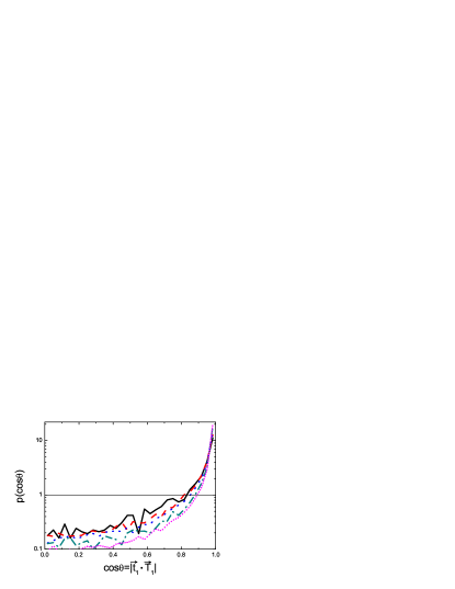
Figure 13: The distribution of the cosine of the angle between the mass tidal field $\vec{T}_{1}$ and the halo tidal field $\vec{t}_{1}$. Adaptive SMS of $M_{h}$ is used to calculate $\vec{T}_{1}$. The results are shown for halos in the same five mass bins as shown in Fig. 1. The horizontal line indicates a random distribution.

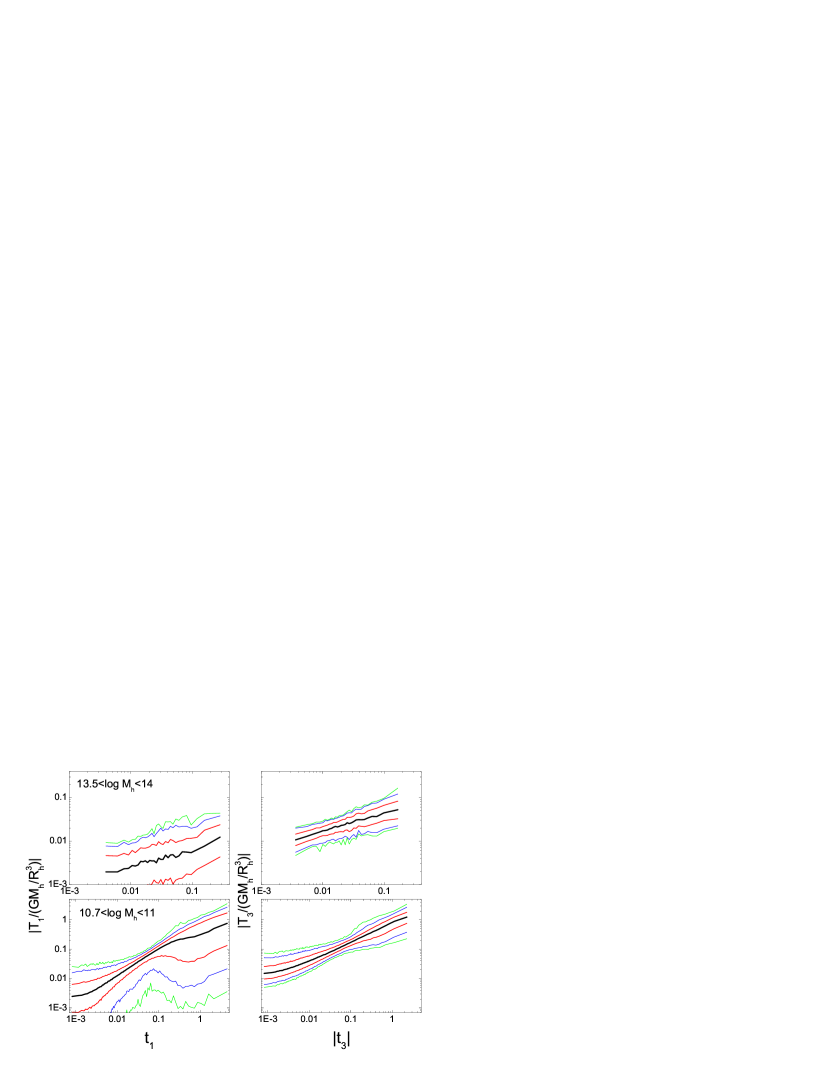
Figure 14: The comparison between the mass tidal field $T_{k}$ and the halo tidal field $t_{k}(k=1,3)$. The latter is calculated using halos with $13.5<log(M_{h}/\,h^{-1}{\rm M_{\odot}})<14$ (upper two panels) and with $10.7<log(M_{h}/\,h^{-1}{\rm M_{\odot}})<11$ (lower two panels). Adaptive SMS of $M_{h}$ is used to calculate $T_{k}$. The black line represents median, while the colored lines are percentiles corresponding to $1\sigma$ (68 per cent, red), $2\sigma$ (95 per cent, blue) and $3\sigma$(99 per cent, green). Note that the lower blue and green lines in the upper-left panel are beyond the scope of the plot, and not plotted.

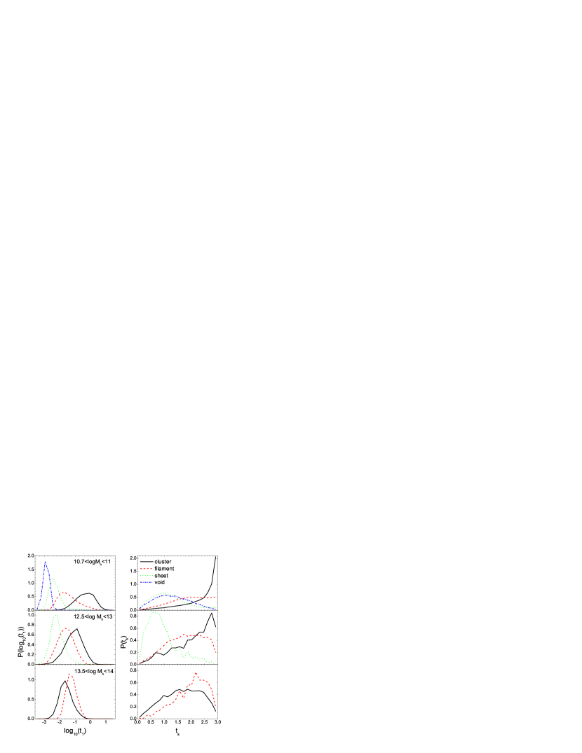
Figure 15: The probability distribution of $t_{1}$ (left panels) and $t_{s}$ (right panels) of halos in three mass ranges and in various types of environment: cluster, filament, sheet and void (see the text for the exact definitions). For the most massive bin, the void population is too small to give a reliable result.

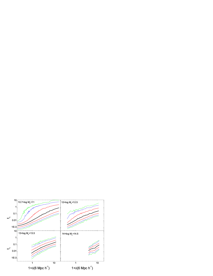
Figure 16: Local overdensity $\delta(6\,h^{-1}{\rm{Mpc}})$ versus halo tidal field $t_{1}$ for halos of various masses. The black line represents median, while the colored lines are percentiles corresponding to $1\sigma$ (68 per cent, red), $2\sigma$ (95 per cent, blue) and $3\sigma$(99 per cent, green).

References

- Allgood et al. (2006) Allgood B., Flores R. A., Primack J. R., Kravtsov A. V., Wechsler R. H., Faltenbacher A., Bullock J. S., 2006, MNRAS, 367, 1781
- Altay, Colberg, & Croft (2006) Altay G., Colberg J. M., Croft R. A. C., 2006, MNRAS, 370, 1422
- Aragón-Calvo et al. (2007) Aragón-Calvo M. A., van de Weygaert R., Jones B. J. T., van der Hulst J. M., 2007, ApJ, 655, L5
- Bamford et al. (2009) Bamford S. P., et al., 2009, MNRAS, 393, 1324
- Bett et al. (2007) Bett P., Eke V., Frenk C. S., Jenkins A., Helly J., Navarro J., 2007, MNRAS, 376, 215
- Binggeli (1982) Binggeli B., 1982, A&A, 107, 338
- Carter & Metcalfe (1980) Carter D., Metcalfe N., 1980, MNRAS, 191, 325
- Chambers, Melott, & Miller (2002) Chambers S. W., Melott A. L., Miller C. J., 2002, ApJ, 565, 849
- Croton, Gao, & White (2007) Croton D. J., Gao L., White S. D. M., 2007, MNRAS, 374, 1303
- D’Onghia & Navarro (2007) D’Onghia E., Navarro J. F., 2007, MNRAS, 380, L58
- Dalal et al. (2008) Dalal N., White M., Bond J. R., Shirokov A., 2008, ApJ, 687, 12
- Davis et al. (1985) Davis M., Efstathiou G., Frenk C. S., White S. D. M., 1985, ApJ, 292, 371
- Desjacques (2008) Desjacques V., 2008, MNRAS, 388, 638
- Diemand, Kuhlen, & Madau (2007) Diemand J., Kuhlen M., Madau P., 2007, ApJ, 657, 262
- Dolag et al. (2006) Dolag K., Meneghetti M., Moscardini L., Rasia E., Bonaldi A., 2006, MNRAS, 370, 656
- Doroshkevich (1970) Doroshkevich A. G., 1970, Ap, 6, 320
- Dressler (1980) Dressler A., 1980, ApJ, 236, 351
- Dutton et al. (2007) Dutton A. A., van den Bosch F. C., Dekel A., Courteau S., 2007, ApJ, 654, 27
- Fakhouri & Ma (2009) Fakhouri O., Ma C.-P., 2009, MNRAS, 394, 1825
- Fall & Efstathiou (1980) Fall S. M., Efstathiou G., 1980, MNRAS, 193, 189
- Faltenbacher et al. (2007) Faltenbacher A., Li C., Mao S., van den Bosch F. C., Yang X., Jing Y. P., Pasquali A., Mo H. J., 2007, ApJ, 662, L71
- Faltenbacher et al. (2009) Faltenbacher A., Li C., White S. D. M., Jing Y.-P., Shu-DeMao, Wang J., 2009, RAA, 9, 41
- Gao, Springel, & White (2005) Gao L., Springel V., White S. D. M., 2005, MNRAS, 363, L66
- Gao et al. (2004) Gao L., White S. D. M., Jenkins A., Stoehr F., Springel V., 2004, MNRAS, 355, 819
- Gao & White (2007) Gao L., White S. D. M., 2007, MNRAS, 377, L5
- Gardner (2001) Gardner J. P., 2001, ApJ, 557, 616
- Hahn et al. (2007) Hahn O., Porciani C., Carollo C. M., Dekel A., 2007a, MNRAS, 375, 489
- Hahn et al. (2007) Hahn O., Carollo C. M., Porciani C., Dekel A., 2007b, MNRAS, 381, 41
- Hahn et al. (2009) Hahn O., Porciani C., Dekel A., Carollo C. M., 2009, MNRAS, 398, 1742
- Harker et al. (2006) Harker G., Cole S., Helly J., Frenk C., Jenkins A., 2006, MNRAS, 367, 1039
- Hetznecker & Burkert (2006) Hetznecker H., Burkert A., 2006, MNRAS, 370, 1905
- Hirata et al. (2007) Hirata C. M., Mandelbaum R., Ishak M., Seljak U., Nichol R., Pimbblet K. A., Ross N. P., Wake D., 2007, MNRAS, 381, 1197
- Hockney & Eastwood (1981) Hockney R. W., Eastwood J. W., 1981, csup.book,
- Holmberg (1969) Holmberg E., 1969, ArA, 5, 305
- Hopkins, Bahcall, & Bode (2005) Hopkins P. F., Bahcall N. A., Bode P., 2005, ApJ, 618, 1
- Ishiyama, Fukushige, & Makino (2008) Ishiyama T., Fukushige T., Makino J., 2008, PASJ, 60, L13
- Jing (1998) Jing Y. P., 1998, ApJ, 503, L9
- Jing, Mo, & Boerner (1998) Jing Y. P., Mo H. J., Boerner G., 1998, ApJ, 494, 1
- Jing et al. (1995) Jing Y. P., Mo H. J., Borner G., Fang L. Z., 1995, MNRAS, 276, 417
- Jing (2002) Jing Y. P., 2002, MNRAS, 335, L89
- Jing & Suto (2002) Jing Y. P., Suto Y., 2002, ApJ, 574, 538
- Jing, Suto, & Mo (2007) Jing Y. P., Suto Y., Mo H. J., 2007, ApJ, 657, 664
- Kang et al. (2007) Kang X., van den Bosch F. C., Yang X., Mao S., Mo H. J., Li C., Jing Y. P., 2007, MNRAS, 378, 1531
- Keselman & Nusser (2007) Keselman J. A., Nusser A., 2007, MNRAS, 382, 1853
- Klypin et al. (1999) Klypin A., Kravtsov A. V., Valenzuela O., Prada F., 1999, ApJ, 522, 82
- Lacey & Cole (1993) Lacey C., Cole S., 1993, MNRAS, 262, 627
- Lee & Erdogdu (2007) Lee J., Erdogdu P., 2007, ApJ, 671, 1248
- Lemson & Kauffmann (1999) Lemson G., Kauffmann G., 1999, MNRAS, 302, 111
- Li, Mo, & Gao (2008) Li Y., Mo H. J., Gao L., 2008, MNRAS, 389, 1419
- Ludlow et al. (2009) Ludlow A. D., Navarro J. F., Springel V., Jenkins A., Frenk C. S., Helmi A., 2009, ApJ, 692, 931
- Macciò et al. (2007) Macciò A. V., Dutton A. A., van den Bosch F. C., Moore B., Potter D., Stadel J., 2007, MNRAS, 378, 55
- Maller, Dekel, & Somerville (2002) Maller A. H., Dekel A., Somerville R., 2002, MNRAS, 329, 423
- Maulbetsch et al. (2007) Maulbetsch C., Avila-Reese V., Colín P., Gottlöber S., Khalatyan A., Steinmetz M., 2007, ApJ, 654, 53
- Mo & Mao (2004) Mo H. J., Mao S., 2004, MNRAS, 353, 829
- Mo, Mao, & White (1998) Mo H. J., Mao S., White S. D. M., 1998, MNRAS, 295, 319
- Mo & White (1996) Mo H. J., White S. D. M., 1996, MNRAS, 282, 347
- Mo et al. (2005) Mo H. J., Yang X., van den Bosch F. C., Katz N., 2005, MNRAS, 363, 1155
- Moore et al. (1999) Moore B., Ghigna S., Governato F., Lake G., Quinn T., Stadel J., Tozzi P., 1999, ApJ, 524, L19
- Navarro, Abadi, & Steinmetz (2004) Navarro J. F., Abadi M. G., Steinmetz M., 2004, ApJ, 613, L41
- Okumura & Jing (2009) Okumura T., Jing Y. P., 2009, ApJ, 694, L83
- Okumura, Jing, & Li (2009) Okumura T., Jing Y. P., Li C., 2009, ApJ, 694, 214
- Paz, Stasyszyn, & Padilla (2008) Paz D. J., Stasyszyn F., Padilla N. D., 2008, MNRAS, 389, 1127
- Peacock & Smith (2000) Peacock J. A., Smith R. E., 2000, MNRAS, 318, 1144
- Peebles (1969) Peebles P. J. E., 1969, ApJ, 155, 393
- Porciani, Dekel, & Hoffman (2002) Porciani C., Dekel A., Hoffman Y., 2002, MNRAS, 332, 339
- Sandvik et al. (2007) Sandvik H. B., Möller O., Lee J., White S. D. M., 2007, MNRAS, 377, 234
- Seljak & Warren (2004) Seljak U., Warren M. S., 2004, MNRAS, 355, 129
- Seljak & Zaldarriaga (1996) Seljak U., Zaldarriaga M., 1996, ApJ, 469, 437
- Shaw et al. (2006) Shaw L. D., Weller J., Ostriker J. P., Bode P., 2006, ApJ, 646, 815
- Shen et al. (2006) Shen J., Abel T., Mo H. J., Sheth R. K., 2006, ApJ, 645, 783
- Sheth, Mo, & Tormen (2001) Sheth R. K., Mo H. J., Tormen G., 2001, MNRAS, 323, 1
- Sheth & Tormen (1999) Sheth R. K., Tormen G., 1999, MNRAS, 308, 119
- Sheth & Tormen (2004) Sheth R. K., Tormen G., 2004, MNRAS, 350, 1385
- Skibba & Sheth (2009) Skibba R. A., Sheth R. K., 2009, MNRAS, 392, 1080
- Springel et al. (2001) Springel V., White S. D. M., Tormen G., Kauffmann G., 2001, MNRAS, 328, 726
- Tinker et al. (2008) Tinker J. L., Conroy C., Norberg P., Patiri S. G., Weinberg D. H., Warren M. S., 2008, ApJ, 686, 53
- Trujillo, Carretero, & Patiri (2006) Trujillo I., Carretero C., Patiri S. G., 2006, ApJ, 640, L111
- van den Bosch (2002) van den Bosch F. C., 2002, MNRAS, 331, 98
- van Haarlem & van de Weygaert (1993) van Haarlem M., van de Weygaert R., 1993, ApJ, 418, 544
- Vitvitska et al. (2002) Vitvitska M., Klypin A. A., Kravtsov A. V., Wechsler R. H., Primack J. R., Bullock J. S., 2002, ApJ, 581, 799
- Wang et al. (2005) Wang H. Y., Jing Y. P., Mao S., Kang X., 2005, MNRAS, 364, 424
- Wang, Mo, & Jing (2007) Wang H. Y., Mo H. J., Jing Y. P., 2007a, MNRAS, 375, 633
- Wang et al. (2007) Wang Y., Yang X., Mo H. J., van den Bosch F. C., 2007b, ApJ, 664, 608
- Wang et al. (2009) Wang H., Mo H. J., Jing Y. P., Guo Y., van den Bosch F. C., Yang X., 2009a, MNRAS, 394, 398
- Wang, Mo, & Jing (2009) Wang H., Mo H. J., Jing Y. P., 2009b, MNRAS, 396, 2249
- Wang et al. (2009) Wang Y., Park C., Yang X., Choi Y.-Y., Chen X., 2009c, ApJ, 703, 951
- Wang et al. (2008) Wang Y., Yang X., Mo H. J., van den Bosch F. C., Weinmann S. M., Chu Y., 2008a, ApJ, 687, 919
- Wang et al. (2008) Wang Y., Yang X., Mo H. J., Li C., van den Bosch F. C., Fan Z., Chen X., 2008b, MNRAS, 385, 1511
- Warren et al. (1992) Warren M. S., Quinn P. J., Salmon J. K., Zurek W. H., 1992, ApJ, 399, 405
- Wechsler et al. (2006) Wechsler R. H., Zentner A. R., Bullock J. S., Kravtsov A. V., Allgood B., 2006, ApJ, 652, 71
- Weinmann et al. (2009) Weinmann S. M., Kauffmann G., van den Bosch F. C., Pasquali A., McIntosh D. H., Mo H., Yang X., Guo Y., 2009, MNRAS, 394, 1213
- Wetzel et al. (2007) Wetzel A. R., Cohn J. D., White M., Holz D. E., Warren M. S., 2007, ApJ, 656, 139
- White (1984) White S. D. M., 1984, ApJ, 286, 38
- Yang, Mo, & van den Bosch (2006) Yang X., Mo H. J., van den Bosch F. C., 2006a, ApJ, 638, L55
- Yang et al. (2006) Yang X., van den Bosch F. C., Mo H. J., Mao S., Kang X., Weinmann S. M., Guo Y., Jing Y. P., 2006b, MNRAS, 369, 1293
- Yang, Mo, & van den Bosch (2003) Yang X., Mo H. J., van den Bosch F. C., 2003, MNRAS, 339, 1057
- Yang et al. (2005) Yang X., Mo H. J., van den Bosch F. C., Jing Y. P., 2005, MNRAS, 356, 1293
- Yang et al. (2007) Yang X., Mo H. J., van den Bosch F. C., Pasquali A., Li C., Barden M., 2007, ApJ, 671, 153
- Zentner (2007) Zentner A. R., 2007, IJMPD, 16, 763
- Zhang et al. (2009) Zhang Y., Yang X., Faltenbacher A., Springel V., Lin W., Wang H., 2009, ApJ, 706, 747
- Zhu et al. (2006) Zhu G., Zheng Z., Lin W. P., Jing Y. P., Kang X., Gao L., 2006, ApJ, 639, L5
.