Gamma-ray spectral properties of mature pulsars: a two-layer model

Abstract

We use a simple two-layer outer gap model, whose accelerator consists of a primary region and a screening region, to discuss $\gamma$-ray spectrum of mature pulsars detected by $Fermi$. By solving the Poisson equation with an assumed simple step-function distributions of the charge density in these two regions, the distribution of the electric field and the curvature radiation process of the accelerated particles can be calculated. In the our model, the properties of the phase-averaged spectrum can be completely specified by three gap parameters, i.e. the fractional gap size in the outer magnetosphere, the gap current in the primary region and the gap size ratio between the primary region and the total gap size. We discuss how these parameters affect the spectral properties. We argue that although the radiation mechanism in the outer gap is curvature radiation process, the observed gamma-ray spectrum can substantially deviate from the simple curvature spectrum because the overall spectrum consists of two components, i.e. the primary region and screening region. In some pulsars the radiation from the screening region is so strong that the photon index from 100MeV to several GeV can be as flat as $\sim 2$. We show the fitting fractional gap thickness of the canonical pulsars increases with the spin down age. We find that the total gap current is about 50 % of the Goldreich-Julian value and the thickness of the screening region is a few percent of the total gap thickness. We also find that the predicted $\gamma$-ray luminosity is less dependent on the spin down power ($L_{sd}$) for the pulsars with $L_{sd}\gtrsim 10^{36}$ erg/s, while the $\gamma$-ray luminosity decreases with the spin down power for the pulsars with $L_{sd}\lesssim 10^{36}$ erg/s. This relation may imply that the major gap closure mechanism is photon-photon pair-creation process for the pulsars with $L_{sd}\gtrsim 10^{36}$ erg/s, while the magnetic pair-creation process for the pulsars with $L_{sd}\lesssim 10^{36}$ erg/s.

1 Introduction

The particle acceleration and high-energy $\gamma$-ray radiation process in the pulsar magnetosphere has been studied with polar cap model (Ruderman & Sutherland 1975; Daugherty & Harding 1982, 1996), the slot gap model (Arons 1983; Muslimov & Harding 2003; Harding et al. 2008) and the outer gap model (Cheng, Ho & Ruderman 1986a,b, hereafter CHRa,b; Hirotani 2008; Takata, Wang & Cheng 2010). All models have assumed that the charged particles are accelerated by the electric field along the magnetic field lines, and that the acceleration region arises in the charge deficit region from the Goldreich-Julian charge density (Goldreich & Julian 1969). The polar cap model assumes the acceleration region near the stellar surface, while the outer gap model assumes a strong acceleration in outer magnetosphere. The slot gap model proposes that the accelerating electric field near the rim of the polar cap can not be completely screened out and the particles are continuously accelerated up to high altitude along the magnetic field lines.

The recent $\gamma$-ray instruments have started to break the bottleneck of study of the high-energy radiation from the pulsar. In particular, the $Fermi$ LAT has detected $\gamma$-ray emissions from 46 pulsars just in one year observation, including 21 radio-selected pulsars, 16 $\gamma$-ray selected pulsars, the Geminga and 8 millisecond pulsars (Abdo et al. 2010a, 2009a,b), while the pulsed radio emissions are reported from several $\gamma$-ray selected pulsars (Camilo et. al. 2009). Romani & Watters (2010) study the pulse profiles of canonical pulsars observed by $Fermi$ LAT. They compute the pulse profiles predicted by the outer gap model and slot gap model with the magnetic field, which is composed of the vacuum dipole field plus the current-induced field. They argued that the outer gap geometry is statistically more consistent with the observations than the slot gap geometry. On the other hand, the present population study has argued that both outer gap and slot gap model may not explain all features of Fermi pulsars; for example, the both model predicts too few young pulsars compared with the $Fermi$ pulsars (c.f. Grenier & Harding 2010). Venter, Harding & Guillemot (2009) fit the pulse profiles of the $Fermi$ detected millisecond pulsars with the geometries predicted by the different emission models. However, they found that the pulse profiles of two out of eight millisecond pulsars cannot be fitted by either the geometries with the outer gap or the caustic models. They proposed a pair-starved polar cap model, in which the multiplicity of the pairs is not high enough to completely screen the electric field above the polar cap, and the particles are continuously accelerated up to high altitude over the entire open field line region.

The observed spectra also allow us to study the site of the $\gamma$-ray emissions in the pulsar magnetosphere. In the first $Fermi$ pulsar catalog (Abdo et al. 2010a), the spectral fits have been done assuming exponential cut-offs. For example, the $Fermi$ LAT measured a detail spectral properties of the Vela pulsar (Abdo et al. 2009c, 2010b). It is found that the observed spectrum is well fitted by a power law plus hyper-exponential cutoff spectral model of the form $dN/dE\propto E^{-a}\exp[-(E/E_{c})^{b}]$ with $b\leq 1$ and $E_{c}\sim 1.5$ GeV. This implies that an emission process in the outer magnetosphere is more favored than that near the stellar surface, which predicts a super exponential cut-off ($b>1$) due to the magnetic pair-creation prosses of the $\gamma$-rays. Furthermore, the detection of the radiation above 25 GeV bands associated with the Crab pulsar by the MAGIC telescope has also implied the emission process in the outer magnetosphere (Aliu et al. 2008).

There is a common idea at least in different outer gap models. Charged deficit regions, in which electric field along magnetic field lines is not zero, exist in the outer magnetospheric regions. The size of outer gap cannot occupy the entire open field line region, because electrons/positrons in the gap are accelerated to extremely relativistic energies and each of these charged particles radiates a very large number of GeV-photons due to the curvature of the magnetic field. Only a small fraction of curvature photons converted into pairs can limit the size of the outer gap (e.g. CHRa,b; Zhang & Cheng 1997). Cheng, Ho & Ruderman (1986a) have argued that a realistic dynamic gap should consist of two regions, i.e. a primary acceleration region of lower part of the gap, where seed current can produce multi-GeV gamma-ray photons, and a screening region of upper part of the gap, where the created electron/positron pairs start to screen out the gap electric field (cf. Fig.12c of CHRa). More detail numerical studies (e.g. Hirotani 2006; Takata et al. 2006) expect that a screening region must exist and in fact most gap current is located in this region.

In this paper we assume a simple two-layer gap structure, which consists of a primary acceleration region and a screening region. The electric field along the magnetic field lines in both regions are not zero but the exact distribution depends on the charge distribution in these two regions. Charged particles accelerated in these regions radiate different curvature spectrum due to the position dependent electric field. The combined spectrum depends sensitively on the charge distribution in these two acceleration regions. The first purpose of this paper is that we explain the photon indics of phase-averaged spectrum of mature pulsars by applying our two-layer outer gap model. Observationally the phase-averaged spectrum above 100 MeV bands of $Fermi$ $\gamma$-ray pulsars can be fit by a single power law plus exponential cut-off form (cf. Abdo et al. 2010a). It is found that the photon index of the power law component distributes between $p\sim 0.5-2.5$ and the distribution has a peak around $p\sim 1.3$ (Abdo et al. 2010a). It is virtually impossible to explain the very soft spectrum with a photon index $p>2$ with a simple curvature emission model by adjusting the curvature radius of a single layer. We will argue that the two-layer model can predict the photon index as flat as $p\sim 2$ due to the overall spectrum consists of the two components, i.e. the curvature radiations from screening region and from the primary region.

The second purpose of this paper is to study the relation between the $\gamma$-ray luminosity and the spin down luminosity. The increases of the $\gamma$-ray pulsars allow us to perform a more detail statistical study. For example, the results of the $Ferm$ will modify the relation between the $\gamma$-ray luminosity ($L_{\gamma}$) and the spin down power ($L_{sd}$), for which $L_{\gamma}\propto L_{sd}^{\beta}$ with $\beta\sim 0.5$ were predicted by $EGRET$ $\gamma$-ray pulsars (Thompson 2004). However, the luminosity $L_{\gamma}$ calculated from the observed flux include ambiguity due to the uncertainties of the distance to the pulsars and of the beaming factor. In this paper, therefore, we theoretically predict $\gamma$-ray luminosity by fitting the properties of the phase-averaged spectrum. This will be important to know the true relation between the $\gamma$-ray luminosity and the spin down power.

This paper is organized as follows. In section 2, we present a simple two dimensional gap model, which ignores the gap structure in the azimuthal direction. By assuming simple step function of the charge distributions in these two acceleration region, we can solve the Poisson equation analytically and obtain the electric field everywhere inside the gap. We calculate the curvature radiation to compare the observed phase-averaged spectrum. In section 3 we discuss how the model parameters affect the spectral properties. We also show the fitting results for the phase-averaged spectrum of the all $Fermi$ detected gamma-ray pulsars except the Crab-like pulsars, whose radiation spectra could be synchrotron-self-Compton process instead of curvature radiation process. In section 4 we discuss the implications of the fitted parameters and deduced parameters. We present a brief conclusion in section 5.

2 Theoretical Model

2.1 Gap structure with two-layer

In addition to pulsar parameters, i.e. rotation period and dipole magnetic field, there are many factors to affect the observed detailed spectrum of individual pulsar, e.g. the phase-resolved spectrum, which depends on the magnetic field structure, the gap structure, the inclination angle, viewing angle etc. However the phase-averaged spectrum is less sensitive to these factors. In fact it can tell us the most crucial factors, which govern the general properties in phase-averaged spectra of all pulsars. It is the aim of this paper to use a simple gap model to describe the acceleration and radiation in the outer gap, and try to identify the key parameters to affect the spectral properties of pulsars. We consider the outer gap accelerator in the magnetic meridian, which includes the rotation axis and the magnetic axis. We divide the outer gap accelerator into two-layers, namely the main acceleration region and the screening region, in the trans-field direction in the magnetic meridian. Fig. 1 illustrates our gap structure with two-layer.

We express the electric potential in the gap as $\Phi=\Phi^{\prime}+\Phi_{0}$, where $\Phi_{0}$ is the co-rotating potential, which satisfies $\bigtriangledown^{2}\Phi_{0}=-4\pi\rho_{GJ}$ with $\rho_{GJ}$ being the Goldreich-Julain charge density. In addition, the potential $\Phi^{\prime}{}$ is the so called non co-rotating potential, which represents the deviation from co-rotating potential and generates the accelerating electric field. Using the Poisson equation $\bigtriangledown^{2}\Phi=-4\pi\rho$, and assuming the derivative of the potential field in the azimuthal direction is much smaller than those in the poloidal plane, we express the Poisson equation of $\Phi^{\prime}$ in the simple 2-dimensional geometry as

$$\left(\frac{\partial^{2}}{\partial x^{2}}+\frac{\partial^{2}}{\partial z^{2}}\right)\Phi^{\prime}=-4\pi(\rho-\rho_{GJ}),$$ (1)

where the coordinates $x$ and $z$ are distance along and perpendicular to the magnetic field lines, respectively. Moreover, we assume that (1) the derivative of the potential field in the trans-field (z) direction is larger than that along (x-direction) the magnetic field line and (2) the variation of the Goldreich-Julian charge density in the trans-field direction is negligible compared with that along the magnetic field line. Although these approximations will be crude for the pulsars that have the gap size in the trans-field direction comparable to the size of the magnetosphere, we may apply these approximations for all pulsars because the typical strength of the electric field in the gap might be described by the solution of the first order approximation. By ignoring the derivative of the potential field along the magnetic field line, we reduce the two-dimensional Poisson equation (1) to one-dimensional form that

$$\frac{\partial^{2}{}}{\partial{z^{2}}}\Phi^{\prime}(x,z)=-4\pi[\rho(x,z)-\rho_{GJ}(x)],$$ (2)

where we approximately express the Goldreich-Julain charge density as $\rho_{GJ}(x)\approx-\frac{\Omega Bx}{2\pi cs}$ (cf. Eqs. 3.2 and 3.3 of CHRa), where $\Omega$ is the angular velocity, $B$ is the magnetic field strength, $s$ is the curvature radius of the magnetic field lines and $s\sim R_{lc}$ with $R_{lc}=c/\Omega$ being the light radius.

To solve the equation (2) we impose the boundary conditions on the lower and upper boundaries. In this study, we consider that the lower boundary is located on the last-open field line, and the upper boundary is located on a fixed magnetic field line. For the lower boundary, the condition that

$$\Phi^{\prime}(x,z=0)=0$$ (3)

is imposed. On the upper boundary, we impose the gap closure conditions that

$$\Phi^{\prime}(x,z=h_{2})=0~{}~{}\mathrm{and}~{}~{}E^{\prime}_{\perp}(x,z=h_{2})=0,$$ (4)

where $E^{\prime}_{\perp}(x,z)=\partial\Phi^{\prime}/\partial z$, and $h_{2}(x)$ is the gap thickness measured from the last-open field line. The gap closure conditions ensure that the total potential (co-rotational potential + non co-rotational potential) field in the gap is continuously connected to the co-rotational potential field outside the gap. We note that three boundary conditions are imposed for the two order differential equation, implying the location of the upper boundary can not be arbitrary chosen, because both Dirichlet-type and Neumann-type conditions are imposed on the upper boundary. In fact, the condition $E^{\prime}_{\perp}(x,z=h_{2})=0$ connects the charge density distribution and the gap thickness $h_{2}(x)$

As illustrated in Fig. 1, we divide the gap into two regions, i.e. the primary acceleration region and the screening region. The main acceleration region is expanding between the last-open field line and the height $z=h_{1}(x)$ (region I in Fig. 1a), and the screening region is expanding between $z=h_{1}(x)$ and $z=h_{2}(x)$ (region II in Fig. 1a). We note that the averaged charge density in the outer gap accelerator must be less than the Goldreich-Julian value, that is $|\rho|<|\rho_{GJ}|$, in the primary acceleration region to arise a strong electric field along the magnetic field line. In the screening region, on the other hand, $|\rho|>|\rho_{GJ}|$ is required to satisfy both boundary conditions in equation (4). Physically speaking, the charge deficit in the primary region is compensated by the charge excess in the screening region.

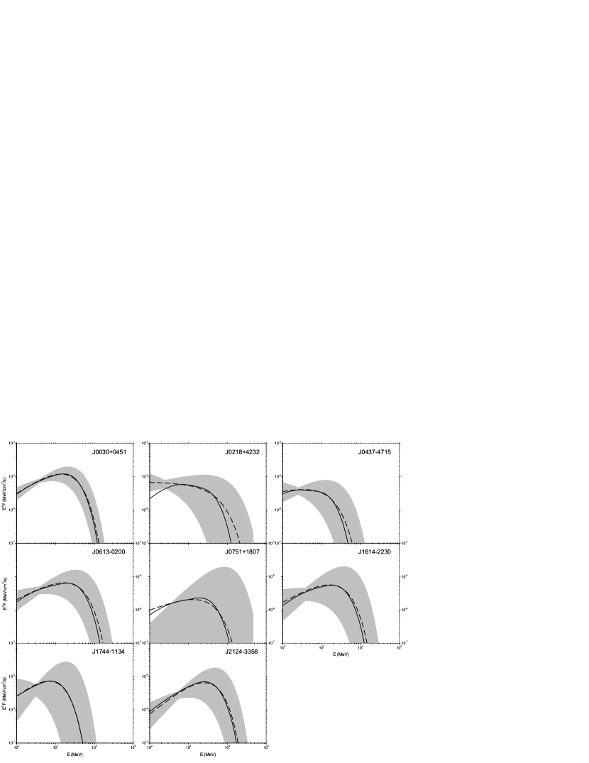
Figure 7: The model results of the millisecond pulsars. The solid lines are model results,the dash lines correspond to the photon indexes, cut off energies and photon fluxes from the $Fermi$ catalogue and the grey strips represent the errors of the three(Abdo et al. 2009a).

As demonstrated by the electrodynamic studies (e.g. figure 7 in Hirotani 2006), (1) the charge density rapidly increases in the trans-field direction at the height where the pair-creation process becomes important, and (2) the increase of the charge density will be saturated around upper boundary because of the screening of the electric field due to the pairs. In this paper, therefore, we describe the distribution of the charge density in the trans-field direction (z-direction) as a step function form (Fig. 1b);

$$\rho(x,z)=\left\{\begin{array}[]{ccc}\rho_{1}(x),&$if$&0\leq z\leq h_{1}(x),\\ \rho_{2}(x),&$if$&h_{1}(x)<z\leq h_{2}(x).\end{array}\right.$$ (5)

We define the boundary $h_{1}(x)$ with a magnetic line as well as $h_{2}(x)$, implying $h_{2}(x)/h_{1}(x)$ is nearly constant along the magnetic field line.

Using the boundary conditions that $\Phi^{\prime}_{z}(z=0)=0$ and $\Phi^{\prime}_{z}(z=h_{2})=0$ and imposing the continuity of the potential field $\Phi^{\prime}_{z}$ and $\partial\Phi^{\prime}_{z}/\partial z$ at the height $h_{1}$, we obtain the solution of the Poisson equation (2) as

$$\Phi^{\prime}(x,z)=-2\pi\left\{\begin{array}[]{ccc}\{\rho_{1}(x)-\rho_{GJ}(x)\}z^{2}+C_{1}z,&$for$&0\leq z\leq h_{1}(x)\\ \{\rho_{2}(x)-\rho_{GJ}(x)\}(z^{2}-h_{2}^{2}(x))+D_{1}(z-h_{2}(x)),&$for$&h_{1}(x)\leq z\leq h_{2}(x)\end{array}\right.$$ (6)

where

$$C_{1}(x)=\frac{(\rho_{1}-\rho_{GJ})h_{1}(h_{1}-2h_{2})-(\rho_{2}-\rho_{GJ})(h_{1}-h_{2})^{2}}{h_{2}}$$

and

$$D_{2}(x)=\frac{(\rho_{1}-\rho_{2})h_{1}^{2}-(\rho_{2}-\rho_{GJ})h_{2}^{2}}{h_{2}}$$

The gap closure condition $E^{\prime}_{\perp}=0$ on the upper boundary provides the relation among the charge densities $(\rho_{1},~{}\rho_{2})$ and the gap thickness $(h_{1},~{}h_{2})$ that

$$[\rho_{2}(x)-\rho_{GJ}(x)]h^{2}_{2}(x)+(\rho_{1}(x)-\rho_{2}(x))h_{1}(x)^{2}=0.$$ (7)

During the fitting process (section 3.2), we will find that the charge density in the main acceleration region is much smaller than that in the screening region, that is, $|\rho_{1}|<<|\rho_{2}|$. This implies that the typical charge density in the screening region is describes as $\rho_{2}(x)\sim\rho_{GJ}(x)/[1-(h_{1}/h_{2})^{2}]$. Namely, both screening conditions $\Phi^{\prime}(z=h_{2})=0$ and $E^{\prime}_{\perp}(z=h_{2})=0$ are satisfied when the charge density in the screening region is proportional to the Goldreich-Julian charge density. In the realistic situation, therefore, we expect that the typical charge density in the screening region is proportional to the Goldreich-Julian charge density. For the charge density, $\rho_{1}$, in the main acceleration region, we also put the charge density proportional to the Goldreich-Julian charge density for simplicity, $\rho_{1}\propto\rho_{GJ}$, because (1) it is expected that the charge density increases along the magnetic field region due to the photon-photon pair-creation process and (2) in fact, the distribution of the charge density in the main acceleration region is less important to the Potential field in the gap (c.f. equation (6)) as long as the charge density $|\rho_{1}|$ is much smaller than $|\rho_{2}|$ and $|\rho_{GJ}|$. We will see in section 3.2, the observed spectrum can be fitted with $\rho_{1}\sim 0.1\rho_{GJ}$ and $\rho_{2}\geq\rho_{GJ}$. Because we consider the case that inclination angle is smaller than $\alpha<90^{\circ}$ and because the outer gap extends beyond the null charge surface, we rewrite the charge density as

$$\frac{\rho-\rho_{GJ}}{\rho_{GJ}}=\left\{\begin{array}[]{ccc}-g_{1},&$if$&0\leq{}z\leq{}h_{1}\\ g_{2},&$if$&h_{1}<z\leq{}h_{2}\end{array},\right.$$ (8)

where $g_{1}>0$, $g_{2}>0$ (cf. Fig. 1c). The accelerating electric field along the magnetic field line, $E^{\prime}_{||}=-\partial\Phi^{\prime}/\partial x$ is described as

$$E^{\prime}_{||}(z)\sim\frac{\Omega B}{cs}\left\{\begin{array}[]{ccc}-g_{1}z^{2}+C^{\prime}_{1}z,&$for$&0\leq z\leq h_{1}(x)\\ g_{2}(z^{2}-h_{2}^{2}(x))+D^{\prime}_{1}(z-h_{2}(x)),&$for$&h_{1}(x)\leq z\leq h_{2}(x)\end{array}\right.$$ (9)

where

$$C^{\prime}_{1}(x)=-\frac{g_{1}h_{1}(h_{1}-2h_{2})+g_{2}(h_{1}-h_{2})^{2}}{h_{2}}$$

and

$$D^{\prime}_{2}(x)=-\frac{(g_{1}+g_{2})h_{1}^{2}+g_{2}h_{2}^{2}}{h_{2}},$$

where we used $\partial(Bh_{2}^{2})/\partial x\sim 0$, $\partial(z/h_{2})/\partial x\sim 0$, $\partial(h_{1}/h_{2})/\partial x\sim 0$ and $\partial s/\partial x\sim 0$.

A particular solution of equation (6) is obtained by specifying any three parameters or their combinations out of four, i.e. $h_{1}$, $h_{2}$, $g_{1}$ and $g_{2}$. In the next section, we fit the observed phase-averaged spectra with the following combination of model parameters, i.e. $h_{2}(R_{lc})/R_{lc}$, $1-g_{1}$ and $h_{1}/h_{2}$, which correspond to the fractional gap size, the physical gap charge density (or current) divided by Goldreich-Julian value in the primary region and the gap size ratio between the primary and screening regions.

2.2 Curvature radiation spectrum

The charged particles are accelerated by the electric field along the magnetic field lines in the gap, and emit $\gamma$-rays via the curvature radiation. The Lorentz factor, $\gamma_{e}$, can be estimated from the condition that $eE^{\prime}_{\parallel}(z)c=l_{cur}(z)$, where $l_{cur}(z)=2e^{2}c\gamma^{4}_{e}(z)/3s^{2}$ is the power of the curvature radiation, as

$$\gamma_{e}(z)=\left[\frac{3}{2}\frac{s^{2}}{e}E^{\prime}_{\parallel}(z)\right]^{1/4}.$$ (10)

For a single particle, the spectrum of curvature radiation is described by

$$F_{cur}^{single}=\frac{\sqrt{3}e^{2}\gamma_{e}}{2\pi{}\hbar{}sE_{\gamma}}F(E_{\gamma}/E_{cur})$$ (11)

where $E_{cur}(z)=(3/2)\hbar{}c\gamma_{e}^{3}(z)/s$ is the characteristic energy of the radiated curvature photon and $F(x)=\int^{\infty}_{x}K_{5/3}(y)dy$, where $K_{5/3}$ is the modified Bessel functions of order 5/3. The total curvature radiation spectrum from the outer gap is computed from

$$F_{cur}(E_{\gamma})=\int n(x,z)F_{cur}^{single}(z)dV,$$ (12)

where $n(x,z)\sim n_{GJ}(x)(1+g(z))$ is the number density, $n_{GJ}(x)=\Omega B(x)/2\pi ce$, and $dV=\delta A_{\perp}(x)dx$ is the volume of the element, where $\delta A_{\perp}(x)$ is the increment area of width $\delta z$. The increment are is calculated as $\delta A_{\perp}(x)\sim 2\pi R_{lc}\delta z(R_{lc})B(R_{lc})/B(x)$, where $\delta z(R_{lc})$ is the width at the light cylinder and we used the magnetic flux conservation that $B(x)\delta A_{\perp}(x)=B(R_{lc})\delta A_{\perp}(R_{lc})\sim 2\pi B_{lc}R_{lc}\delta z(R_{lc})$.

The total flux received at Earth is

$$F(E_{\gamma})=\frac{1}{\Delta{\Omega}d^{2}}F_{cur}(E_{\gamma}),$$ (13)

where $d$ is the distance of the pulsar and $\Delta{\Omega}$ is the solid angle.

3 Results

3.1 Properties of the curvature spectra with the gap structures

Basically we have three independent fitting parameters, i.e the fractional gap size defined by $f\equiv h_{2}(R_{lc})/R_{lc}$, the number density (current) in the primary region ($1-g_{1}$) and the ratio between the thicknesses of primary region and total gap size $h_{1}/h_{2}$. Qualitatively the fractional gap size mainly determines the total potential drop in the gap and the strength of the accelerating field, and hence it affects the intensity and the cut-off energy of the curvature radiation. We will see that the number density ($1-g_{1}$) in the primary region determines the slope of the curvature spectrum below the cut-off energy and the ratio ($h_{1}/h_{2}$) controls the spectral break in lower energy bands around 100 MeV. In below we give the quantitative description how these three parameters affect the spectrum.

Fig. 2 summarizes the dependency of the curvature spectra on the gap thickness. The lines present the spectra with the fractional gap thickness of $f$=0.8 (solid line), 0.6 (dashed line), 0.4 (dotted line) and 0.2 (dashed-dotted line). The results are for $1-g_{1}=0.10$, $h_{1}/h_{2}=0.933$ and the parameters of the Geminga pulsar. We can see in Fig. 2 that the spectral properties are sensitive to the gap thickness. Specifically, the intensity increases with the gap fractional thickness. This is because the total potential drop in the gap and therefore magnitude of the accelerating electric field are proportional to the square of the gap thickness ($\Phi^{\prime}\propto f^{2}$), as equations (6) and (9) imply. Therefore, the predicted flux of the curvature radiation from the gap is approximately proportional to $E_{\gamma}^{2}F\propto\Phi^{\prime}\times N\propto f^{3}$, where we used that the total number of the particles (or current) in the gap is proportional to $N\propto f$. Fig. 2 also shows that the spectrum becomes hard with increase of the fractional gap thickness. From the equations (9) and (10), we can see that the typical energy of the curvature photons is proportional to $E_{\gamma}\propto(3/2)\hbar c\gamma_{e}^{3}/s\propto f^{3/2}$, implying the cut-off energy in spectrum increases with the fractional gap thickness as Fig. 2 shows.

Fig. 3 shows how the charge density, $\rho=(1-g_{1})\rho_{GJ}$, of the primary region affects the curvature spectrum. The lines represent the curvature spectra for $1-g_{1}=0.30$ (solid line), $0.10$ (dashed line), 0.05 (dotted line) and $0.01$ (dashed-dotted line). The results are for $f=0.76$, $h_{1}/h_{2}=0.933$ and the parameters of the Geminga pulsar are used. Qualitatively speaking, the number density in the primary region determines the slope of the spectrum below the cut-off energy. We can find in Fig. 3 (e.g. dashed-dotted line) that the spectrum is divided into two components, that is, higher and lower energy components. The higher energy component ($E_{\gamma}\gtrsim 1$ GeV) comes from the primary region, where the charge density is smaller than the Goldreich-Julain charge density, while the other one ($E_{\gamma}\lesssim 1$ GeV) originates from the screening region, where the charge density exceeds the Goldreich-Julain charge density. Because the accelerating electric field in the primary region is stronger than that in the screening region, the Lorentz factor of the particles and the resultant typical energy of the curvature photons are larger in the primary region than in the screening region.

The screening condition, $(h_{2}/h_{1})^{2}=1+g_{1}/g_{2}$ (c.f. Eq.7), implies a larger number density (corresponding to larger $g_{2}$) in the screening region is required for a smaller number density (corresponding to larger $g_{1}$) in the primary region. In such a case, if the number density of the primary region is much smaller than Goldreich-Julian value, the energy flux of the curvature radiation from the primary region becomes small compared with that from the screening region, as indicated by the dashed-dotted line in Fig 3. With the present model, therefore, number density in the primary region, and resultant ratio of the total numbers of particles in the primary and the screening regions mainly determines the slope of the spectrum below the cut-off energy. Fig. 3 also shows that the cut-off energy in the spectra in GeV energy bands decreases as the charge density in the primary region (or $1-g_{1}$) increases. This is because the deviation from the Goldreich-Julian charge density becomes small as the charge density increases, implying that the accelerating electric field and the resultant typical energy of the curvature photons decrease with increasing of the charge density.

Fig.4 summarizes the dependency of the properties of the curvature spectrum on the ratio of the thicknesses between the primary region and the screening region, $h_{1}/h_{2}$. The lines represent the curvature spectra for $h_{1}/h_{2}=0.70$ (solid line), $0.80$ (dashed line), 0.90 (dotted line) and $0.96$ (dashed-dotted line) with $f=0.76$, $1-g_{1}=0.1$ and the parameters of the Geminga pulsar. We note that the increase of the ratio $h_{1}/h_{2}$ corresponds to the decrease of the thickness of the screening region ($h_{2}-h_{1}$) relative to the primary region. In the present model, the ratio $h_{1}/h_{2}$ determines the energy width between the spectral cut-off in GeV band and the spectral break in 100 MeV bands, because the curvature spectrum of the primary region has an energy peak at several GeV, while that of the screening region shows an energy peak at several hundred MeV. In the dashed-dotted line in Fig. 4 ($h_{1}/h_{2}=0.96$), for example, the spectral cut-off appearing at several GeV is a result of the emissions from the primary region, while the spectral break seen around 200 MeV is produced by the emissions from the screening region. As the ratio decreases, on the other hand, the position of the spectral break in lower energy shifts to higher energy (e.g. $\sim$500 MeV for $h_{1}/h_{2}=0.90$), and the energy width between the cut-off energy and the spectral break energy decreases. This is because the thickness of the screening region ($h_{2}-h_{1}$) relative to that of the primary region ($h_{1}$) becomes thick as the ratio decreases, implying the flux of the emissions from the screening region increases and its spectrum becomes hard. For the ratio $h_{1}/h_{2}=0.70$ (solid line in Fig. 4), the emissions from the screening region dominates the emissions from the primary region.

3.2 Fitting Results

We fit the phase-averaged spectra of the 42 $\gamma$-ray pulsars measured by the $EGRET$ and $Fermi$ telescopes with the present model. For the observed spectra, we use information reported in the first $Fermi$ catalogue (Abdo et al. 2010a), in which the observed data were fit with a single power law plus exponential cut-off form. In our fitting, we do not include the Crab-like young pulsars (e.g. the Crab pulsar, PSR J1124-5916) because the radiation mechanism of the Crab-like pulsars are synchrotron-self-Compton process instead of curvature radiation process (Cheng, Ruderman & Zhang 2000; Takata & Chang 2007). In the Crab-like pulsars their soft photon density is sufficiently high so that most curvature photons from the outer gap will be converted into pairs within the light cylinder and the observed gamma-rays resulting from the inverse Compton scattering of the synchrotron photons of secondary pairs. This radiation process differs from what we have considered in this paper and therefore we will not consider them.

As discussed in section 3.1, our fitting parameters are the fractional gap thickness $f$, the charge density in the primary region, $1-g_{1}$, and the ratio $h_{1}/h_{2}$. In fact, given observed phase-averaged spectrum can be uniquely fit with one set of $(f,1-g_{1},h_{1}/h_{2})$ with a small uncertainty. The model fitting was proceeded as following. First, we deduced the typical fractional gap thickness, $f$, from the observed intensity and the cut-off energy, because the fractional gap thickness $f$ greatly affects the intensity and the cut-off energy as Fig. 2 shows. For the next step, we fit the spectral slope below the cut-off energy with the charge density in the primary region, $1-g_{1}$, which mainly controls the slope of the calculated spectrum as Fig. 3 shows. Finally, we determined $h_{1}/h_{2}$, which controls the spectral width between the cut-off energy in several GeV and the spectral break energy in lower energy bands.

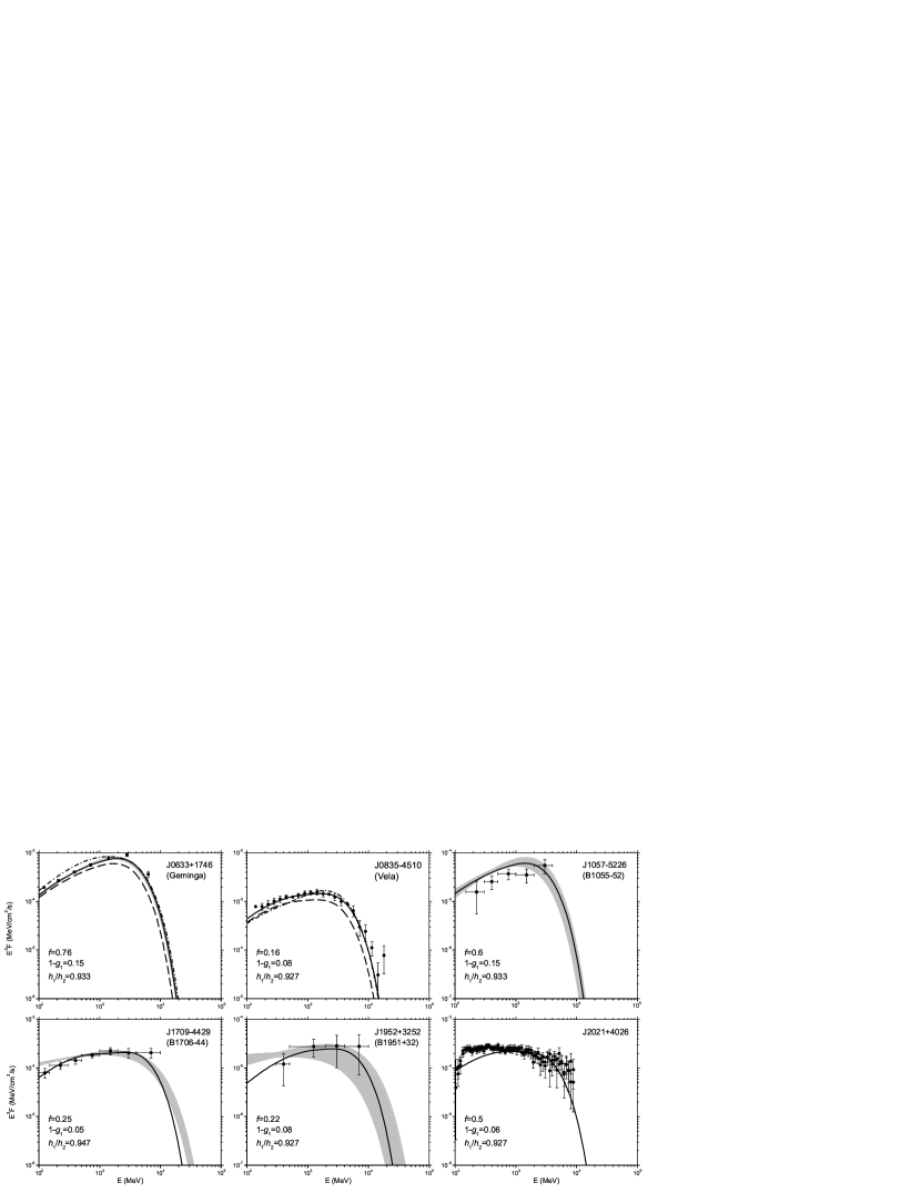
Figure 5: The model results of 6 canonical pulsars. The solid lines represent the best fitting model spectra with the fitting parameters listed in each panel. The circles are the observed data from the $Fermi$ LAT, which are taken from Abdo et al. (2009d) for the Vela pulsar and Trep et al. (2010) for J2021+4026. The boxes are the observed data from $EGERT$ (Fierro 1995). The dotted lines in the panels of the Geminga and the Vela pulsars are results for the fractional gap thickness ($f=0.7$ for the Geminga and 0.145 for the Vela) about 10 % difference than the best fitting fractional gap thickness, while the dashed-dotted lines are results for $1-g_{1}$ (0.13 for the Geminga and 0.1 for the Vela) and $h_{1}/h_{2}$ (0.867 for the Geminga and 0.967 for the Vela) about 10-20 % difference than the best fitting parameters.

Fig. 5 presents the fitting results with the observed data for the 6 canonical pulsars. The data points are taken from the EGRET observations (Fierro, 1995) for the Geminga, PSRs J057-5226,J1709-4229 and J1952+3252, and from the $Fermi$ observations for the Vela (Abdo et al. 2009c and 2010b) and PSR J2021+4206 (Trep et al. 2010). The grey strips represent the errors of the photon index, cut-off energy and intensity measured by the $Fermi$ observations. The solid lines represent the best fit spectra with the fitting parameters listed in each panel and in Table 1. We use the dashed and dashed-dotted lines in the panels of the Gemiga and Vela pulsars to preset how the best fit parameters include the uncertainties. The dotted lines are results for the fractional gap thickness ($f=0.7$ for the Geminga and 0.145 for the Vela) about 10 % difference than the best fitting values, while the dashed-dotted lines are results for $1-g_{1}$ (0.13 for the Geminga and 0.1 for the Vela) and $h_{1}/h_{2}$ (0.867 for the Geminga and 0.967 for the Vela) about 10-20 % difference than the best fitting values. It is obvious that both dashed and dashed-dotted lines can not explain the observed data, implying the fitting parameters include uncertainties of about 10 % for the Geminga and Vela pulsars.

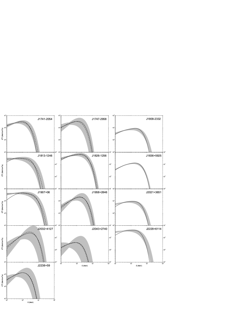
Figure 6: The model results of 28 canonical pulsars. The solid lines are model results, the dash lines correspond to the photon indexes, cut off energies and photon fluxes from the $Fermi$ catalogue and the grey strips represent the errors of the three(Abdo et al. 2009a).

Figs 6 and 7 compare fitting results with the $Fermi$ observations for the 28 canonical pulsars and 8 millisecond pulsars, respectively. The solid line and dashed line are corresponding to the model spectra and the observations, respectively. The grey strips represent the errors of the observations. In Figs 6-7, we can see that the present model can reproduce well the observations, although there is a small discrepancy between the model and the observations around 100 MeV energy bands for some pulsars (such as PSRs J1907+06 and J2229+6144).

In Table 1, we summarize the observed pulsar parameters (second-fifth columns) and the fitting parameters (sixth-ninth columns). Fig. 8 plots the fitted fractional gap thickness as a function of the spin down age $\tau$. We find in Fig. 8 that the fitted fractional gap size $f_{fit}$ (sixth column) is between 0.1-0.9 and is bigger than the estimated fractional gap size of the Crab pulsar (e.g. CHRb estimated $f_{Crab}\sim 0.05$). We can see a clear trend in Fig. 8 that the fractional gap thickness for the canonical pulsars increases with the spin down age. This is expected because the potential drop of the pulsar decreases as the spin down age increases, implying a larger fractional gap thickness is required to accelerate the particles to emit several GeV $\gamma$-ray photons via the curvature radiation process. For the millisecond pulsars, it is required more number of sample to argue the relation between the fractional gap size and the spin down age.

In seventh column of Table 1 we can see that the current in the primary region is roughly $\sim 10\%$ of the Goldreich-Julian current. This is important because if the gap current in this region is too large then accelerating electric field is not strong enough to accelerate the gap electrons/positrons to sufficiently high Lorentz. Consequently multi-GeV photons cannot be generated and pair creation process cannot take place.

The ratio between the primary region and the total gap size $h_{1}/h_{2}$ is less than but very closed to unity. This indicates that the screening region is very thin and is only a few percents of the total gap size. This is expected because although the mean free path ($\lambda$) of photon-photon pair-creation is longer than the light cylinder radius in the case of mature pulsars, the thickness of the screening region is substantially reduced by the photon multiplicity ($N_{\gamma}$) and it can be estimated as

$$h_{2}-h_{1}\approx\frac{\lambda^{2}}{sN_{\gamma}^{2}}$$ (14)

(cf. equation 5.7 and C21 of CHRa). Taking $\lambda\sim 10^{3}R_{lc}$, $s\sim R_{lc}\sim 10^{9}cm$ and $N_{\gamma}\sim 10^{4}$, $h_{2}(R_{lc})-h_{1}(R_{lc})\sim 10^{7}~{}\mathrm{cm}<<h_{2}(R_{lc})\sim 10^{8}-10^{9}$cm. Also the magnetic pair-creation near the stellar surface could supply the screening pairs within a thin layer (Takata et al. 2010).

In order to match the observed gamma-ray flux, we need to introduce one more fitting parameter, i.e. $\Delta\Omega d^{2}$ (ninth column), which is the product of gamma-ray solid angle and the distance to the pulsar. Using the observed distance (fourth column) and the fitting $\Delta\Omega d^{2}$, we estimate the solid angle $\Delta\Omega_{fit}$ (twelfth column). We can see that the averaged value of the deduced solid angle $\Delta\Omega_{fit}$ is order of unity, which is usually assumed. On the other hand, some $\gamma$-ray pulsars are required a solid angle much larger ($>10$) or smaller ($<0.1$) solid angle than the averaged value. This would reflect the effects of the viewing geometry. The fitting solid angle much larger (or smaller) than the mean value may imply that the pulsars are observed with a viewing angle which cuts through the emission region where the intensity is much smaller (or larger) than the mean intensity.

For the observed distance to pulsar, we can see that first of all the error of the observed distance is usually quite large and secondly there are some pulsars without the measured distance. Therefore if the solid angle of gamma-ray pulsars is the same, which is usually assumed to be unity, then we can use the theoretical predicted power and the observed flux to predict the distance to the pulsar, which is listed in the last column of Table 1.

4 Discussion

In Table 1 we deduce the averaged gap current in units of the Goldreich-Julain value (tenth column). In addition to show that the curvature radiation emitted by the accelerated charged particles can consistently explain the observed spectrum of mature pulsars detected by $Fermi$, it is interesting to note that from Table 1 that the gap current is roughly constant. Specifically, the variation of the gap current is less than 20% and the gap current is around 50-60% of the full Goldreich-Julian current. Although it is not easily explain why the total current in the gap is close to half of Goldreich-Julian value, this result appears qualitatively reasonable because if the current is very closed to the Goldreich-Julian current, the electric field will be substantially reduced. Consequently the charged particles cannot be accelerated to extremely relativistic to emit multi-GeV photons and hence pair creation process cannot occur. In fact we speculate that the gap may operate in a dynamical format, namely, the gap can begin with an almost charge starvation state, and then charged particles are accelerated to extremely relativistic and emit $10^{4}-10^{5}$ photons per particle across the gap. A small fraction of these photons are converted into pairs, which can almost immediately quench the gap, and the current in this stage is almost full Goldreich-Julian current. Since particles and photons are all moving in speed of lights, the on/off time scales of these two stages should be very similar and which may be order of $R_{lc}/c$. After averaging over time, it may not be surprised to have a time average gap current about 50% of the Goldreich Julian value. If there were good time resolution, this speculation predicts that there is a time variability in the $\gamma$-ray intensity with a time scale of $R_{lc}/c$. This may be an evidence of the pair-creation process in the pulsar magnetosphere, which maintains the global electric circuit of the star.

The predicted $\gamma$-ray luminosity ($L^{fit}_{\gamma}$), for each pulsar is listed in eleventh column of Table 1, where we use $L^{fit}_{\gamma}=f^{3}_{fit}L_{sd}$ with $L_{sd}=(2\pi)^{4}B_{s}^{2}R_{s}^{6}/6c^{3}P^{4}$ being the spin down luminosity. We note that uncertainties of the predicted $\gamma$-ray luminosity is small because the uncertainties of the fitting parameters is small, say about 10 %, as discussed in section 3.2. In Fig. 9, the predicted $\gamma$-ray luminosity is plotted as a function of the spin down power $L_{sd}$. We can see a trend in Fig. 9 that the predicted $\gamma$-ray luminosity shows less dependency on the spin down power for the pulsars with $L_{sd}\gtrsim 10^{36}$ erg/s, while $L_{\gamma}$ decreases with the spin down power for the pulsars with $L_{sd}\lesssim 10^{36}$ erg/s. This change of the dependency of the $\gamma$-ray luminosity on the spin down power may be caused by switching the gap closure process. In fact, the solid and dashed lines in Fig. 9 represent the relation predicted by the outer gap model with different gap closure processes as follows.

Zhang & Cheng (1997) have argued that when the pulsars cool down, the cooling X-rays may not be sufficient to convert the curvature photons emitted by the accelerated particles into pairs to restrict the growth of the outer gap. They suggest that however the X-rays emitted by the heated polar cap due to the return current can provide a self-consistent mechanism to restrict the fractional size of the gap as

$$f_{ZC}=0.32P_{-1}^{26/21}B_{12}^{-4/7},$$ (15)

where $P_{-1}$ is the rotation period in units of 0.1s. This model predicts the $\gamma$-ray luminosity is related with the spin down luminosity as $L_{\gamma}\propto L_{sd}^{1/14}B_{12}^{1/7}\sim L_{sd}^{1/14}$, which is represented by the solid line in Fig.9. This less dependency on the spin down luminosity may explain the behavior of the predicted $\gamma$-ray luminosity of the pulsars with $L_{sd}\gtrsim 10^{36}$ erg/s.

Recently Takata et al. (2010) argue that since the electric field decreases rapidly from the null charge surface to the inner boundary, where the gap electric field must vanish, the radiation loss cannot be compensated by the acceleration of the local electric field. When this occurs the Lorentz factor of the incoming electrons/positrons is determined by the equating the radiation loss time scale and the particle crossing time scale. It is interesting to note that the characteristic photon energy of curvature radiation is independent of pulsar parameters and is given by $m_{e}c^{2}/\alpha_{f}\sim 100\rm MeV$, where $\alpha_{f}$ is the fine structure constant.

They further argue that these 100MeV photons can become pairs by magnetic pair creation process. These secondary pairs can continue to radiate due to synchrotron radiation and the characteristic energy of synchrotron photons is of order of several MeV. The photon multiplicity is easily over $10^{5}$ per each incoming particle. Such cascade process has also been considered before (e.g. Cheng & Zhang 1999). For a simple dipolar field structure, all these pairs should move inward and they cannot affect the outer gap. However they argue that the existence of strong surface local field (e.g. Ruderman 1991, Arons 1993) has been widely suggested. In particular if the field lines near the surface, instead of nearly perpendicular to the surface, are bending sideward due to the strong local field. The pairs created in these local magnetic field lines can have an angle bigger than 90^∘, which results in an outgoing flow of pairs. In fact it only needs a very tiny fraction (1-10) out of $10^{5}$ photons creating pairs in these field lines, which are sufficient to provide screening in the outer gap when they migrate to the outer magnetosphere.

They estimate the fractional gap thickness when this situation occurs as

$$f_{m}=0.25KP_{-1}^{1/2},$$ (16)

where $K\propto B_{m,12}^{-2}s_{7}$ is the parameter to characterize the local parameters, e.g. $B_{m,12}$ and $s_{7}$ are the local magnetic field in units of $10^{12}$G and the local curvature radius in units of $10^{7}$cm. From this estimate they predict that the gamma-ray luminosity is related to the spin down power as $L_{\gamma}\propto L_{sd}^{5/8}$, which is represented by the dashed-line in Fig 9. This gap closure process may explain the relation between the predicted $\gamma$-ray luminosity and the spin down power for the pulsars with $L_{sd}\lesssim 10^{36}$ erg/s, as Fig. 9 indicates.

5 Conclusion

In this paper, we applied the two-layer outer gap model to fit the observed phase-averaged spectra of the 42 $\gamma$-ray pulsars detected by the $Fermi$ telescope. Our gap structure consists two parts, which are the primary acceleration region and the screening region (Fig. 1). In the primary acceleration region, the charge density is less than the Goldreich-Julian charge density ($|\rho|<|\rho_{GJ}|$), while in the screening region, the charge density exceeds $\rho_{GJ}$ to screen out the accelerating electric field. Assuming a step function of distribution of charge density in the direction perpendicular to the magnetic field lines, we solve the Poisson equation to obtain the accelerating electric field in the gap. We fit the observed phase-averaged spectrum with the three fitting parameters, that is, the fractional gap thickness $f$, the number density of the primary region ($1-g_{1}$), and the ratio of the thicknesses of the primary and the secondary regions, $h_{1}/h_{2}$. We demonstrated that the gap thickness affects the position of the cut-off energy (several GeV) appeared in the curvature spectrum, as Fig.2 shows. We also showed that the number density of the primary region and the resultant ratio of the number densities between the primary and the screening region determine the slope of the spectrum below the cut-off energy (Fig. 3), and that the ratio $h_{1}/h_{2}$ mainly affects the position of the spectral break at 100 MeV bands (Fig.4), which is caused by the emissions from the screening region. With two-layer mode, the observed soft spectrum with the photon index of $\sim 2$ for the some pulsars can be explained by the overall spectrum consists of the two components, i.e. the curvature radiations from screening region and from the primary region. Our fitting results show that the fractional gap thickness for the canonical pulsars tends to increases with the spin down age, as Fig 8. shows. The observations can be fit by the ratio $h_{1}/h_{2}$ smaller than but close to unity, implying the screening region is only a few percent of total gap thickness. The present model predicts the gap current is about 50 % of the Goldreich-Julain value. We found that the predicted $\gamma$-ray luminosity shows less dependency on the spin down power for the pulsars with $L_{sd}\gtrsim 10^{36}$ erg/s, while it decreases with the spin down power for pulsars with $L_{sd}\lesssim 10^{36}$ erg/s (Fig. 9). We discussed the relation of the $\gamma$-ray luminosity and the spin down power with the gap closure mechanisms of Zhang& Cheng (1997), which predict $L_{\gamma}\propto L_{sd}^{1/14}$ and of Takata et al. (2010), which predicts $L_{\gamma}\propto L_{sd}^{5/8}$.

While the present simple model can be applied to discuss the observed phase-averaged spectra, a three-dimensional model should be required to discuss the observed light curves and the phase-resolved spectra. The detail properties of the observed light curves (e.g. number of the peak and phase of peak) and the phase-resolved spectra will reflect the three-dimensional distributions of the number density of particle and electric field in the gap. For example, the $Fermi$ telescope revealed the third peak, whose position depends on the energy bands, in the light curve of the Vela pulsar (Abdo et al. 2009d, 2010). The third peak in GeV energy bands, which has not been expected by the previous emission models, will be understood with a detail three-dimensional analysis. In the subsequent papers, therefore, we will extend the present two-dimensional analysis into a three-dimensional one, and fit the phase resolved spectra and the energy-dependent light curve for the individual pulsar.

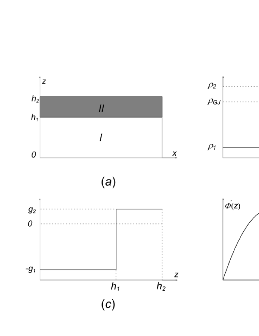
Figure 1: Schematic view of the gap structure. (a)The structure of the outer gap with two-layer. The regions $I$ and $II$ are the primary region and the screening region respectively. (b)The distribution of the charge density in the trans-field ($z$) direction in the gap. (c)The distribution of the $g(z)$ in $z$-direction in the gap. (d)The distribution of the $\Phi^{\prime}{}(z)$, and the accelerating electric field $E^{\prime}_{||}(z)\propto\Phi^{\prime}{}(z)$.

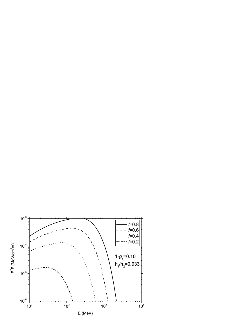
Figure 2: The effects of $f$ on the shape of the spectrum of the curvature radiation. The results are for $1-g_{1}=0.1$ and $h_{1}/h_{2}=0.933$. The parameters of Geminga are used.

Figure 3: The effect of the charge density of the main acceleration region, $1-g_{1}$, on the shape of the spectrum, where $h_{1}/h_{2}=0.933$ and $f=0.76$ are used. The parameters of Geminga are used.

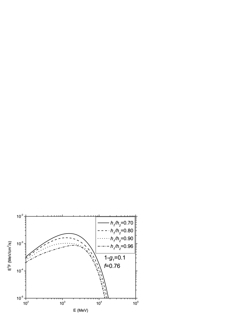
Figure 4: The effect of $h_{1}/h_{2}$ on the shape of the spectrum with the $1-g_{1}=0.1$ and $f=0.76$. The parameters of Geminga are used.

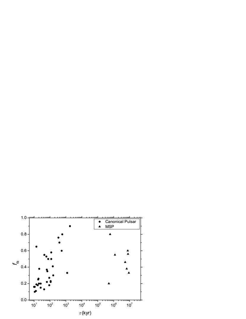
Figure 8: The fitting fractional gap thickness as a function of the spin down age. The circle and triangle represent for the canonical and millisecond pulsars, respectively.

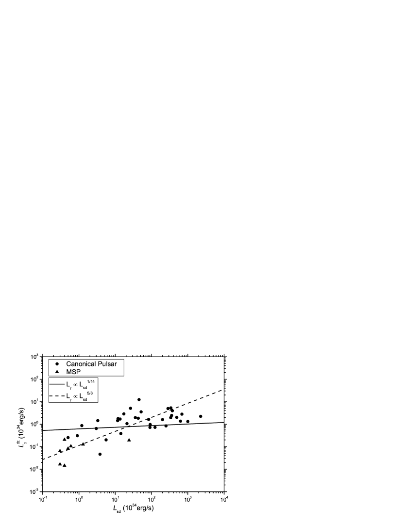
Figure 9: The predicted $\gamma$-ray luminosity as a function of the spin down power. The circle and triangle represent for the canonical and millisecond pulsars, respectively. The solid and dashed lines represent the models by Zhang & Cheng (1997) and Takata et al. (2010), respectively.

Table 1: Parameters

	Observed Parameters				Fitting Parameters				Deduced Parameters
Name	$P$ (ms)	$B_{12}$	$d^{obs}$ (kpc)	$F_{100}^{obs}$(10-8ph cm-2s-1)	$f_{fit}$	$1-g_{1}$	$h_{1}/h_{2}$	$\Delta{\Omega}d^{2}$ (kpc2)	$\eta_{gap}$	$L_{\gamma}^{fit}$ (1033erg/s)	$\Delta{\Omega}_{fit}$	$d(\Delta{\Omega}=1)$
J0007+7303∗	316	10.6	$1.4\pm 0.3$	$30.7\pm 1.3$	0.65	0.06	0.967	4.508	0.538	124.1	$2.3^{+1.42}_{-0.74}$	2.12
J0248+602	217	3.44	2-9	$3.7\pm 1.8$	0.37	0.10	0.953	6.875	0.561	10.63	0.08-1.72	2.62
J0357+32∗	444	1.9	$\cdots$	$10.4\pm 1.2$	0.80	0.12	0.927	0.72	0.577	2.56	$\cdots$	0.85
J0631+1036	288	5.44	0.75-3.62	$2.8\pm 1.2$	0.55	0.10	0.953	18	0.561	28.78	1.37-32	4.24
J0633+0632∗	297	4.84	$\cdots$	$8.4\pm 1.4$	0.53	0.10	0.947	4.81	0.562	17.72	$\cdots$	2.19
J0633+1746	237	1.59	$0.250^{+0.120}_{-0.062}$	$305.3\pm 3.5$	0.76	0.15	0.933	0.125	0.590	14.49	$2^{+1.54}_{-1.09}$	0.35
J0659+1414	385	4.34	$0.288^{+0.033}_{-0.027}$	$10\pm 1.4$	0.23	0.05	0.920	0.12442	0.545	0.4624	$1.5^{+0.32}_{-0.29}$	0.35
J0742-2822	167	1.67	$2.07^{+1.38}_{-1.07}$	$3.18\pm 1.2$	0.30	0.08	0.920	4.2849	0.559	3.861	$1^{+3.28}_{-0.64}$	2.07
J0835-4510	89.3	3.40	$0.287^{+0.019}_{-0.017}$	$1061\pm 7.0$	0.16	0.08	0.927	0.08237	0.557	28.18	$1^{+0.13}_{-0.12}$	0.29
J1028-5819	91.4	1.21	$2.33\pm 0.70$	$19.6\pm 3.1$	0.27	0.09	0.947	1.9544	0.557	16.38	$0.36^{+0.38}_{-0.15}$	1.40
J1048-5832	124	3.48	$2.71\pm 0.81$	$19.7\pm 3.0$	0.20	0.10	0.947	1.98291	0.562	16.08	$0.27^{+0.28}_{-0.11}$	1.41
J1057-5226	197	1.08	$0.72\pm 0.2$	$30.45\pm 1.7$	0.60	0.15	0.933	0.72576	0.590	6.48	$1.4^{+1.28}_{-0.54}$	0.85
J1418-6058∗	111	4.37	2-5	$27.7\pm 8.3$	0.16	0.10	0.940	2.2	0.564	20.27	0.09-0.55	1.48
J1420-6048	68.2	2.38	$5.6\pm 1.7$	$24.2\pm 7.9$	0.11	0.06	0.947	1.2544	0.543	13.31	$0.04^{+0.04}_{-0.02}$	1.12
J1459-60∗	103	1.6	$\cdots$	$17.8\pm 3.4$	0.22	0.05	0.927	1.45	0.543	9.786	$\cdots$	1.20
J1509-5850	88.9	0.90	$2.6\pm 0.8$	$8.7\pm 1.4$	0.41	0.09	0.960	7.098	0.554	35.49	$1.05^{+1.14}_{-0.44}$	2.66
J1709-4429	102	3.04	1.4-3.6	$149.8\pm 4.1$	0.25	0.05	0.947	0.63	0.538	53.28	0.05-0.32	0.79
J1718-3825	74.7	0.99	$3.82\pm 1.15$	$9.1\pm 5.8$	0.18	0.11	0.947	2.48071	0.567	7.29	$0.17^{+0.18}_{-0.07}$	1.58
J1732-31∗	197	2.24	$\cdots$	$25.3\pm 3.0$	0.50	0.11	0.933	1.62	0.570	17	$\cdots$	1.27
J1741-2054∗	414	2.31	$0.38\pm 0.11$	$20.3\pm 2.0$	0.70	0.10	0.960	0.361	0.559	3.087	$2.5^{+2.45}_{-1.00}$	0.60
J1747-2958	98.8	2.46	2-5	$18.2\pm 4.2$	0.15	0.10	0.953	1.2	0.561	8.471	0.05-0.30	1.10
J1809-2332∗	147	2.24	$1.7\pm 1.0$	$49.5\pm 3.0$	0.35	0.07	0.947	0.7225	0.548	18.44	$0.25^{+1.22}_{-0.15}$	0.85
J1813-1246∗	48.1	0.92	$\cdots$	$28.1\pm 3.5$	0.13	0.05	0.927	1.25	0.543	13.75	$\cdots$	1.12
J1826-1256∗	110	3.64	$\cdots$	$41.8\pm 4.1$	0.19	0.07	0.947	1.28	0.548	24.56	$\cdots$	1.13
		Observed Parameters				Fitting Parameters				Deduced Parameters
Name	$P$ (ms)	$B_{12}$	$d^{obs}$ (kpc)	$F_{100}^{obs}$(10-8ph cm-2s-1)	$f_{fit}$	$1-g_{1}$	$h_{1}/h_{2}$	$\Delta{\Omega}d^{2}$ (kpc2)	$\eta_{gap}$	$L_{\gamma}^{fit}$ (1033erg/s)	$\Delta{\Omega}_{fit}$	$d(\Delta{\Omega}=1)$
J1836+5925∗	173	0.51	$<0.8$	$65.6\pm 1.8$	0.90	0.10	0.940	0.32	0.564	8.748	$>0.5$	0.56
J1907+06∗	107	3.09	$\cdots$	$40.25\pm 3.8$	0.26	0.05	0.920	3.81	0.545	49.92	$\cdots$	1.95
J1952+3252	39.5	0.48	$2.0\pm 0.5$	$17.6\pm 1.9$	0.22	0.08	0.927	6.6	0.558	39.82	$1.65^{+1.28}_{-0.59}$	2.57
J1958+2846∗	290	7.95	$\cdots$	$7.65\pm 1.6$	0.38	0.20	0.967	8	0.607	19.64	$\cdots$	2.83
J2021+3651	104	3.18	$2.1^{+2.1}_{-1.0}$	$67.35\pm 4.4$	0.18	0.07	0.927	0.7938	0.553	19.71	$0.18^{+0.48}_{-0.14}$	0.89
J2021+4026∗	265	3.84	$1.5\pm 0.45$	$152.6\pm 4.9$	0.50	0.06	0.927	0.28125	0.548	14.5	$0.125^{+0.13}_{-0.05}$	0.53
J2032+4127∗	143	1.68	1.6-3.6	$6\pm 2.3$	0.58	0.30	0.953	25.2	0.658	51.31	1.94-9.84	5.02
J2043+2740	96.1	0.35	$1.80\pm 0.54$	$2.41\pm 0.90$	0.33	0.12	0.933	2.961	0.575	2.012	$0.9^{+0.94}_{-0.37}$	1.71
J2229+6114	51.6	2.00	0.8-6.5	$32.6\pm 2.2$	0.10	0.07	0.940	2	0.549	22.5	0.05-3.125	1.41
J2238+59∗	163	4.04	$\cdots$	$6.8\pm 1.8$	0.20	0.15	0.967	3.64	0.582	7.224	$\cdots$	1.91
Millisecond pulsars
	Observed Parameters				Fitting Parameters				Deduced Parameters
Name	$P$ (ms)	$B_{8}$	$d^{obs}$ (kpc)	$F_{100}^{obs}$(10-8ph cm-2s-1)	$f_{fit}$	$1-g_{1}$	$h_{1}/h_{2}$	$\Delta{\Omega}d^{2}$ (kpc2)	$\eta_{gap}$	$L_{\gamma}^{fit}$ (1033erg/s)	$\Delta{\Omega}_{fit}$	$d(\Delta{\Omega}=1)$
J0030+0451	4.9	2.27	$0.3\pm{}0.09$	$5.83\pm{}0.78$	0.60	0.12	0.947	0.36	0.572	0.648	$4^{+4.16}_{-1.63}$	0.6
J0218+4232	2.3	4.14	2.5-4	$6.2\pm 1.7$	0.20	0.05	0.920	1.17	0.545	1.92	0.07312-0.1872	1.08
J0437-4715	5.8	2.9	$0.1563\pm{}0.0013$	$3.65\pm{}0.84$	0.38	0.05	0.927	0.12215	0.543	0.165	$5^{+0.08}_{-0.08}$	0.35
J0613-0200	3.1	1.76	$0.48^{+0.19}_{-0.11}$	$3.38\pm 0.85$	0.46	0.08	0.947	0.8064	0.553	1.265	$3.5^{+2.39}_{-1.70}$	0.898
J0751+1807	3.5	1.5	$0.6^{+0.6}_{-0.2}$	$1.35\pm 0.66$	0.56	0.07	0.947	1.62	0.548	1.054	$4.5^{+5.63}_{-3.38}$	1.272
J1614-2230	3.2	1.2	$1.27\pm{}0.39$	$2.89\pm 1.2$	0.55	0.10	0.933	0.80645	0.566	0.832	$0.5^{+0.54}_{-0.21}$	0.898
J1744-1134	4.1	1.8	$0.357^{+0.043}_{-0.035}$	$4.3\pm 1.6$	0.33	0.15	0.953	0.15294	0.585	0.1438	$1.2^{+0.28}_{-0.24}$	0.391
J2124-3358	4.9	2.4	$0.25^{+0.25}_{-0.08}$	$1.95\pm 0.49$	0.80	0.15	0.953	2	0.585	2.048	$32^{+37.2}_{-24}$	1.414

Note. — The first column is the name of the pulsar, the pulsar with ”^∗” means it is a $\gamma$-ray selected pulsar, which was detected by $Fermi$ blind search. The second to fifth column are observed parameters: periods, surface magnetic fields in units of $10^{12}$G, observed distances and the photon flux respectively. The data of these four columns are from the pulsar catalogue of the $Fermi$ LAT(Abdo et al. 2010a). $g_{1}$, $h_{1}/h2$, $f_{fit}(R_{lc})$ and $\Delta{\Omega}d^{2}$ are fitting parameters. $\eta_{gap}\equiv\frac{\rho}{\rho_{GJ}}=\frac{(1-g_{1})h_{1}+(1+g_{2})(h_{2}-h_{1})}{h_{2}}$ is the average gap current in units of Goldreich-Julian current. $L_{\gamma}^{fit}=f_{fit}^{3}L_{sd}$ is the $\gamma$-ray luminosity of the model result. $\Delta{\Omega}_{fit}\equiv\Delta{\Omega}d^{2}/d_{obs}^{2}$, the errors are due to the errors of the distances. The $d(\Delta{\Omega=1})$ is the predicted distance in units of kpc, it is obtained from the fitting parameter $\Delta{\Omega}d^{2}$, when $\Delta{\Omega}=1$.

References

- Abdo (2010a) Abdo A.A. et al., 2010a, ApJS, 187, 460
- Abdo (2010b) Abdo A.A. et al., 2010b, ApJ, 713, 154
- Abdo (2009) Abdo A.A. et al., 2009a, Sci., 325, 848
- Abdo (2009) Abdo A.A. et al., 2009b, Sci., 325, 840
- Abdo (2009) Abdo A.A. et al., 2009c, ApJ, 696, 1084
- Aliu (2009) Aliu E. et al., 2008, Sci, 322, 1221
- Arons (1993) Arons J., 1993, ApJ, 408, 160
- Arons (1983) Arons J., 1983, ApJ, 266, 215
- Camilo (2009) Camilo F. et al., 2009 ApJ, 705, 1
- Cheng (1986a) Cheng K.S., Ho C. & Ruderman M. 1986a, ApJ, 300, 500
- Cheng (1986b) Cheng K.S., Ho C. & Ruderman M. 1986b, ApJ, 300, 522
- Cheng (2000) Cheng K.S., Ruderman, M & Zhang L., 2000, ApJ, 537, 964
- Cheng (1999) Cheng K.S. & Zhang L., 1999, ApJ, 515, 337
- Daugherty (1982) Daugherty J.K. & Harding A.K., 1982, ApJ, 252, 337
- Daugherty (1996) Daugherty J.K. & Harding A.K., 1996, ApJ, 458, 278
- Fierro (1995) Fierro J.M., 1995, PhD thesis, Stanford Univ
- Goldreich (1969) Goldreich P. & Julian W.H., 1969, ApJ, 157, 869
- Harding (2008) Harding A.K., Sterm J.V., Dyks J. & Frackowiak M., 2008, ApJ, 608, 1378
- Hirotani (2008) Hirotani K., 2008, ApJ, 688L, 25
- Hirotani (2006) Hirotani K., 2006, ApJ, 652, 1475
- Romani (2010) Romani R.W. & Watters, K.P., 2010, ApJ, 714, 810
- Muslimov (2003) Muslimov A.G. & Harding A.K., 2003, ApJ, 588, 430
- Ruderman (1991) Ruderman M.A., 1991, ApJ, 366, 261
- Ruderman (1975) Ruderman M.A. & Sutherland P.G., 1975, ApJ, 196, 51
- Takata (2006) Takata J., Shibata S., Hirotani K. & Chang H.-K., 2006, MNRAS, 366, 1310
- Takata (2007) Takata J. & Chang H.-K., 2007, ApJ, 670, 677
- Takata (2010) Takata J, Wang Y & Cheng K.S., 2010, ApJ, 715, 1318
- Thompson (2004) Thompson D.J., 2004, in Cheng K.S., Romero G.E., eds, Cosmic Gamma Ray Sources. Dordrecht, Kluwer, p. 149
- Trep (2010) Trep L., Hui C.Y., Cheng K.S., Takata J., Wang Y., Liu Z.Y. & Wang N., 2010, MNRAS, in press
- Venter (2009) Venter C., Harding A.K. & Guillemot L., 2009, ApJ, 707, 800
- Zhang (1997) Zhang L. & Cheng K.S., ApJ, 1997, 487, 370