Entanglement renormalization of anisotropic XY model

Abstract

The renormalization group flows of the one-dimensional anisotropic XY model and quantum Ising model under a transverse field are obtained by different multiscale entanglement renormalization ansatz schemes. It is shown that the optimized disentangler removes the short-range entanglement by rotating the system in the parameter space spanned by the anisotropy and the magnetic field. It is understood from the study that the disentangler reduces the entanglement by mapping the system to another one in the same universality class but with smaller short range entanglement. The phase boundary and corresponding critical exponents are calculated using different schemes with different block sizes, look-ahead steps and truncation dimensions. It is shown that larger truncation dimension leads to more accurate results and that using larger block size or look-ahead step improve the overall calculation consistency.

The real-space renormalization-group (RSRG),Wilson (1971); *PhysRevB.4.3184; *RevModPhys.47.773 revolving around the coarse-graining and rescaling transformation, has been proven to be a very useful tool in the understanding of the critical phenomenons and the quantum many-body system, whose difficulty lies in the exponential growing of the Hilbert space with the system size. The original RSRG, introduced by Wilson based on the block spin idea,Kadanoff (1966); *RevModPhys.39.395 addresses the problem by dividing the system into blocks and truncating the block Hilbert space to a subspace spanned by a few eigenstates of the lowest energies.Wilson (1971); *PhysRevB.4.3184; *RevModPhys.47.773 Later, White suggested that one should consider the interplay between the block and its environment in the truncating and promoted the density matrix renormalization group (DMRG).White (1992); *PhysRevB.48.10345 In DMRG algorithm, the states to be retained are the eigenstates with the largest eigenvalues of the reduced density matrix of the ground state of the block and its environment.White (1992); *PhysRevB.48.10345 Since the reduced density matrix measures the entanglement between the block and its environment, it is later understood that the performance of DMRG depends on the entanglement in the ground state.Vidal et al. (2003); *PhysRevLett.91.147902; *PhysRevLett.92.087201; *PhysRevLett.93.227205 Unfortunately, near the quantum critical point, the ground state has large entanglement and hence one needs large truncated dimension to get accurate result. To solve this problem, Vidal proposed a new entanglement renormalization method, multiscale entanglement renormalization ansatz (MERA),Vidal (2007); *PhysRevLett.101.110501; *PhysRevA.79.040301; Evenbly and Vidal (2009) by introducing an additional unitary transformation $U$, the disentangler, which acts on the boundary of the adjacent blocks to remove the short-range entanglement (SRE) before performing the coarse-graining. MERA has been shown to be a successful numerical scheme in a lot of different physics systems, such as one-dimensionalEvenbly and Vidal (2009) and two-dimensional quantum spin system,Evenbly and Vidal (2009); *PhysRevLett.104.187203 interacting Fermions,Corboz et al. (2010) boundary critical phenomena.Silvi et al. (2010); *arXiv:0912.1642 However, there are still some very important problems about MERA that need to be answered, such as how exactly does the disentangler remove SRE, what is the difference among the different MERA scheme? In this paper, we try to understand these problem by applying MERA to study the anisotropic XY model (AXY)under a transverse field.

The Hamiltonian of AXY is defined as $H=\sum_{i}H_{i,i+1}$, withLieb et al. (1961); *PhysRev.127.1508

$$H_{i,i+1}=-{J\over 2}[(1+\gamma)S^{x}_{i}S^{x}_{i+1}+(1-\gamma)S^{y}_{i}S^{y}_{i+1}]-{h\over 2}(S^{z}_{i}+S^{z}_{i+1})\,,$$ (1)

where $i$ is the site index, $S^{\alpha}=\sigma^{\alpha}/2\ (\alpha=x,y,z)$ are the spin components represented by the Pauli matrix $\sigma^{\alpha}$. $J$, $\gamma$ and $h$ stand for the interaction strength, anisotropy of the interaction and transverse field respectively. In the limits of $\gamma=0$ and $1$, the model becomes the XY model and the Ising model in a transverse field (ITF) respectively. The model is exact soluble by using the Jordan-Wigner and Fourier transformations.Barouch et al. (1970); *PhysRevA.3.786 The ground state of AXY in the regime $0<\gamma\leq 1$ belongs to the quantum Ising model universality class.Barouch et al. (1970); *PhysRevA.3.786 The system exhibits three critical lines at $x_{c}(\gamma)=h_{c}(\gamma)/J=\pm 1$ and $\gamma_{c}=0$. Under weak magnetic field ($|x|=|h/J|<1$), the system is in the ferromagnetic phase. When the field increases to the critical value $x=x_{c}(\gamma)=1$, the system undergoes a quantum phase transition (QPT) then turns into the paramagnetic phase when the field further increases above the critical value. Due to the exact solubility and rich physics, AXY and its special case ITF have been extensively studied to understand the nature of QPT, especially the role of the entanglement in QPT.Osborne and Nielsen (2002); Patané et al. (2007); Zhou et al. (2008) It also provides a test field for new numerical schemes.Drzewiński and van Leeuwen (1994); Drzewiński and Dekeyser (1995) The phase diagrams and the critical exponents of AXY and ITF have been obtained using various RSRG and DMRG schemes. In this paper, we study these models by using different MERA schemes.

MERA can be understood as a quantum circuit or renormalization group (RG) transformation.Vidal (2007); *PhysRevLett.101.110501; *PhysRevA.79.040301; Evenbly and Vidal (2009); Verstraete et al. (2009) Here we focus on the RG point of view. As demonstrated in Fig. 1, the system is divided into blocks of $n$ sites, the RG transformations are performed by applying a serial of disentanglers $U$ and isometries $W$ on these blocks. The coarse-graining is implemented by the isometry $W$, which maps the Hilbert space on a $n$-site block into a new space on a coarse-grained site. The new Hilbert space is truncated to a subspace of dimension $\chi$ small enough for one to carry out the calculation, but large enough to represent the system faithfully. The purpose of the disentangler is to remove SRE so that one can use small $\chi$ to get accurate result even in the critical regime. The applying of the disentangler $U$ and the isometry $W$ lifts the system on the original sites to a new system on the coarse-grained sites. By comparing the properties of the Hamiltonian or the ground state of the original system and the corresponding coarse-grained version, one can get the renormalized parameters that define the coarse-grained system. Repeating the process one then gets a well defined RG flow. The RG flow of the entanglement was obtained for the ground state of QIT and AXY models using a special MERA scheme targeting at the max entangled states by removing the unentangled modes.Vidal (2007) It was shown that the disentangler indeed reduces the inter-block entanglement. However, this special MERA scheme is designed to obtain max entangled states but not suitable for the general purpose. Moreover, the RG flow in the traditional sense, i.e. the change of the physics parameters that define the system Hamiltonian under the RG transformation, and how the disentangler affects the flow remain to be further studied.

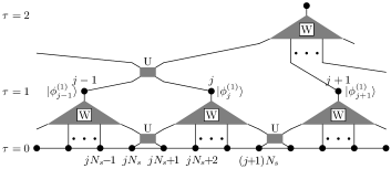
Figure 1: MERA scheme

In order to target the ground state, we assume that the ground state takes the form of the block mean field stateQuinn and Weinstein (1982) after $\tau$-layer coarse-graining,

$$|\Phi^{(\tau)}\rangle=\Pi_{j}|\phi^{(\tau)}_{j}\rangle$$ (2)

where $|\phi^{(\tau)}_{j}\rangle$, whose form does not depend on $j$, is a wave-function defined on the $j$-th block at the $\tau$-th coarse-grained layer. In MERA’s language, we use translational invariant MERA, but set the truncation dimension of the top ($\tau+1$-th) layer isometry to be $1$. The disentanglers and isometries corresponding to this block mean field state are optimized by the algorithm for the translational invariant MERA presented in Ref. Evenbly and Vidal, 2009. For the coarse-grained Hamiltonian to have same symmetries as the original one, the disentanglers and the isometries are chosen to preserve the spatial reflection symmetry and global parity symmetry.Sukhwinder Singh (2009) It should be noted that even though we might use more than one layer of coarse-graining to obtain the ground state in the form of Eq. (2), the RG flow is solely determined by the disentangler $U$ and $W$ at the first layer. Our RG scheme is similar to the Born-Oppenheimer RG scheme used in Ref. Quinn and Weinstein, 1982 with multiple look-ahead steps. However, we do not need to introduce some artificial parameters to describe the slow mode, which is nothing but the effect of the inter-block interaction and is naturally and self-consistently taken into account in MERA scheme. Like the original Born-Oppenheimer RG scheme, $\tau$ can be viewed as look-ahead step. The scale invariant MERAVidal (2007); *PhysRevLett.101.110501; *PhysRevA.79.040301; Evenbly and Vidal (2009) used to study the critical system can be seen as an approximation of infinite look-ahead steps. In the following we will discuss the results for different MERA schemes, such as with/without disentangler, different block size $n$, look-ahead step $\tau$. For simplicity, the schemes are denoted by a string ‘$n\tau xZ$’, where $n$ is the block size, $\tau$ is the look-ahead step, $x$ can be 1 for the simple block mean field state or $\infty$ for the scale invariant scheme. $Z$ is ‘D’ for schemes with or ‘I’ for without disentangler respectively.

We first focus on the simplest case when only two states, one with even parity and the other with odd parity, are retained so that we can track the RG flow analytically. Under the restriction of symmetry requirement, the disentangler takes the form of $U=U_{\text{E}}+U_{\text{O}}$ with $U_{\text{E}}$ and $U_{\text{O}}$ apply on the even and odd parity subspace respectively. For the disentangler acts on sites 0 and 1, $U_{\text{E}}$ and $U_{\text{O}}$ take the following two possible forms

$$U_{\text{E}} = \left\{\begin{array}[]{l}{\cos\theta\over 2}(1+\sigma_{0}^{z}\sigma_{1}^{z})+i{\sin\theta\over 2}(\sigma_{0}^{x}\sigma_{1}^{y}+\sigma_{0}^{y}\sigma_{1}^{x})\\ {\cos\theta\over 2}(\sigma_{0}^{z}+\sigma_{1}^{z})+{\sin\theta\over 2}(\sigma_{0}^{x}\sigma_{1}^{x}-\sigma_{0}^{y}\sigma_{1}^{y})\\ \end{array}\right.$$ (5)

$$U_{\text{O}} = (1-\sigma_{0}^{z}\sigma_{1}^{z})/2\text{\ \ or \ \ }(\sigma_{0}^{x}\sigma_{1}^{x}+\sigma_{0}^{y}\sigma_{1}^{y})/2\,.$$ (6)

The disentangler keeps the form of the AXY Hamiltonian $H_{i,i+1}$ on the boundary sites unchanged, but maps the anisotropy $\gamma$ and magnetic field $x=h/J$ to $\gamma^{\prime}$ and $x^{\prime}$, with

$$\gamma^{\prime} = \gamma\cos 2\theta+x\sin 2\theta,$$ (7)

$$x^{\prime} = -\gamma\sin 2\theta+x\cos 2\theta.$$ (8)

That is, it rotates the vector $(\gamma,x)$ in the parameter space by $2\theta$. Since SRE depends on these parameters,Lagmago Kamta and Starace (2002); Osborne and Nielsen (2002) it is possible for the disentangler to remove the inter-block entanglement by suitable rotation. It is noted that even if one starts from ITF model in which $\gamma=1$, applying of disentangler renders it to general AXY model with $\gamma\not=1$ unless one is limited to $\theta=0$, which is equivalent to without applying disentangler. This is quite different from the previous RSRG schemes for ITF where the RG transformations do not change the form of ITF Hamiltonian. The change from ITF to AXY should not affect the calculation of the critical properties since the anisotropy is irrelevant term and AXY belongs to same universality class for for all regime $0<\gamma\leq 1$. From this aspect, MERA actually provides a possible way for one to identify the universality class.

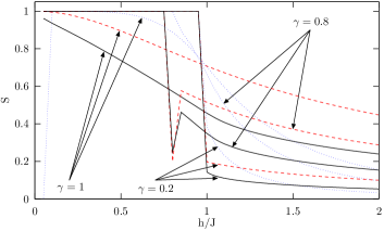
Figure 2: (Color online) Concurrence of ground state of the two qubit AXY system at different RG stages as functions of magnetic field under different anisotropies: Dashed (red) curves: Original system; Solid (black) curves: After applying the optimal disentangler; Dotted (blue) curves: After one RG transformation.

To see the effect of the disentangler on SRE, we use the concurrence of the ground state of the two qubit systemLagmago Kamta and Starace (2002) composed of the spins on the two adjacent sites. It is known that the concurrence of the two qubit system stays at 1 for $\eta=\sqrt{\gamma^{2}+x^{2}}<1$ and decreases as $\gamma/\eta$ when $\eta$ is larger than one. At exactly $\eta=1$, the concurrence is $1-\gamma/2$ which is a local minimal when $x<\gamma^{3}(4-\gamma)/(2-\gamma)^{2}$.Lagmago Kamta and Starace (2002) Strictly speaking, this concurrence can only measure the entanglement of the isolated two qubit system and should not be regarded as the exact SRE between the two boundary spins. Nevertheless, it provides some qualitative information of SRE and the simple form enables one to understand the role of disentangler analytically. In Fig. 2, we plot the concurrence of the ground state of the two qubit system after the applying of the disentangler for different magnetic fields and anisotropies. For comparison, we also plot the concurrence of the original and coarse-grained two-qubit system. The figure clear shows that the disentangler indeed reduces SRE. Analytically, the optimized $\theta$ is larger than zero when $\eta<1$ and continually approaches to negative values when $\eta$ becomes larger than 1. When $\eta=1$, the optimized $\theta$ is about $0$. One can see from these results that, the optimized disentangler reduces SRE by mapping the system to a new one of the same universality class but with smaller entanglement.

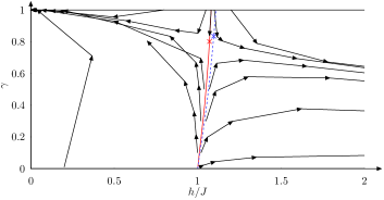
Figure 3: (Color online) RG flows and phase boundaries obtained from different MERA schemes: Solid black lines with arrow, RG flows from 321D scheme; Solid red curve, phase boundary with 321D scheme; Dashed blue curve, phase boundary with 521D scheme. The critical fixed points are marked by cross.

In Fig. 3, we present the flows in the parameter space under RG transformation and the phase boundary defined by the flows. It is seen that the system has three critical lines at $\gamma=0,x\leq 1$, and $0<\gamma\leq 1,x=x_{c}(\gamma)$ that divide the parameter space $-1\leq\gamma\leq 1$ and $-\infty<x<\infty$ into four parts (since the diagram is symmetrical under $x\rightarrow-x$ and $\gamma\rightarrow-\gamma$, only one part is shown in the figure). Starting from $\gamma>0,x<x_{c}(\gamma)$, RG transformations eventually bring the system to the attractive point $\gamma=1,x=0$ which represents the ferromagnetic phase. While staring from $\gamma>0,x>x_{c}(\gamma)$, it is brought to another fixed point at $\gamma=0,x=\infty$, corresponding to the paramagnetic phase. On the critical line $x=x_{c}(\gamma)$, there is another critical fixed point $0<\gamma=\gamma_{c}\leq 1$. In Table. 1, we list the critical field for $\gamma\simeq 0$ and 1, critical fixed point and some of the critical exponents obtained from 321D scheme. To show the effect of the disentangler, we also list the corresponding results from 321I scheme, which is identical to 321D except that it does not have disentangler, for comparison. One can easy see that adding the disentangler greatly improves the accuracy of the phase boundary and the critical exponents. For example, without the disentangler, the critical field for Ising model is $x_{c}(1)=1.291$ from 321I scheme while with disentangler it is $1.081$. Moreover, these two schemes give different critical fixed points. For 321I schemes, it is $\gamma_{c}=1,x_{c}=1.291$ which is in consistence with the results from standard RSRG and DMRG schemes. However, with disentangler the critical fixed point becomes $\gamma_{c}=0.801,x_{c}=1.071$ for 321D scheme, clearly deviates from that of 321I scheme. The difference in the positions of critical fixed point is a result purely from the disentangler. It also reveals the role of the disentangler in MERA scheme. Namely, the disentangler changes the position the critical fixed point so that the critical system has smaller SRE and can be better represented by small truncation dimension.

The number of the look-ahead step also affects the accuracy. Generally speaking, larger $\tau$ leads to more accurate results but also larger calculation cost. The optimal choice of $\tau$ can be understood from RG and MERA point of view. The wave-function obtained here is a variational one in the product state form. For system that is not close to the critical regime, a few RG transformations should bring the system to the attractive fixed points such as the paramagnetic or ferromagnetic states, whose ground states are the simple product states. Therefore for system away from critical regime, one can use the wave-function in the form of Eq. (2) with small $\tau$ to represent the ground state accurately. Further increasing $\tau$ should only have small effect since the disentanglers and isometries on the top layers would be identical to each other as the system flows to the trivial fixed points. As the system approaching the critical regime, more RG transformations, hence larger $\tau$, are need to bring the system to the product state. Exactly at the critical points, one needs infinite $\tau$ to represent the ground state faithfully using the product state form. In this case, the disentanglers and isometries on the lowest layers are different from each other since the irrelevant terms are different at different RG stages. As one goes up to the higher layer, these irrelevant terms eventually vanish and the system is brought to the critical fixed point. After that, the disentanglers and isometries will be the same for different layers due to the scale invariance. In practice, one can choose a few “free” layers with different disentanglers and isometries then put scale invariant layers on top of the “free” layers. This scale invariant MERA scheme was used to study the properties of various critical systems.Evenbly and Vidal (2009) It was believed that the scale invariant MERA can only be applied to the critical system. However, we argue that since it can be seen as an approximation of MERA with infinite look-ahead steps, one can expect that the scale invariant MERA can represent the system faithfully in the vicinity of the fixed points not matter they are critical or noncritical.

The results with different look-ahead steps are listed in Table 1. At first glance, it seems that different look-ahead steps do not lead to any significant differences in phase boundary and critical exponents. Product state MERA and scale invariant MERA also only give slightly difference in the phase diagram and critical exponents. However, further studies show that larger look-ahead steps and scale invariant scheme improve the accuracy on the other physics quantities, such as the susceptibility, and the consistency of these quantities. For example, the susceptibility, proportional to $-\partial^{2}E_{g}(h)/\partial h^{2}$, should diverge at the phase transition point. However, with $321$D scheme, the susceptibility of ITF merely has a smooth peak at $x=0.95$, which is far away from the critical field determined by the RG flow. As one increases the look-ahead step, the peak sharpens and moves towards the critical field. Using scale invariant MERA further improves the consistency. Using $33\infty$D scheme, the position of the peak already consists with the critical field. Further increasing of “free” layer number further sharpens the peak but has little effect on the position.

We now turn to the accuracy of RG for different block size. In Table. 1 we list the critical fields and critical exponents obtained from different block sizes. It is known that the accuracy of the traditional RSRG can be improved by increasing the block size.Jullien et al. (1978); Quinn and Weinstein (1982); Iglói (1993); Drzewiński and van Leeuwen (1994); Drzewiński and Dekeyser (1995) This fact is justified by the results without disentangler. As shown in the table, $x_{c}(1)$ is improved from 1.291 of the 3-site block scheme to 1.233 of the 5-site block scheme. However with the disentangler, increasing the block size leads to slightly worse results, at least when the block size is small. Both the phase boundary and the critical exponents are getting a bit worse off when the block site increases from 3 to 5 and further to 7. However, like increasing the look-ahead step, increasing the block size also improves the consistency of the overall calculations. The $51\infty$D and $52\infty$D schemes product the susceptibility peaks similar to that from $32\infty$D and $33\infty$D schemes respectively. From this aspect, the increasing of block size does improve the overall accuracy in some sense. Following the logics of Ref. Iglói, 1993, without the disentangler, the accuracies of the critical field and the critical exponents increase asymptotically as inverse of the block size or logarithm of the block size. Since the results obtained from MERA with disentangler are always better than that without, it is expected that the accuracy on the phase boundary and critical exponents can be improved by increasing the block size when the block is large enough. However, increasing block size to improve the accuracy of the phase boundary and critical exponents is not a good strategy due to the following two reasons. One is the non-monotonic dependence of the accuracy on the block size and the formidable calculation cost of MERA scheme with larger block size. The other reason is that, as the block size increases, the disentangler becomes close to identity and the difference between the results with and without disentangler gradually diminishes. This trend can be seen by comparing the results from $321$D, $321$I, $521$D and $521$I schemes listed in Table. 1. In practice, use small block size but larger truncation dimension is a more feasible approach for one dimensional system with short range interactions. The optimal scheme for this kind of system is ternary MERA, but the other block sizes are also acceptable when desired.

	Exact	$321$D	$321$I	$32\infty$D	$521$D	$521$I	$32\infty$D(4)
$x_{c}(0)$	1	1	1	1	1	1	1
$x_{c}(1)$	1	1.081	1.291	1.092	1.110	1.233	1.001
$\gamma_{c}$		0.801	1	0.803	0.835	1
$x_{c}(\gamma_{c})$	1	1.071	1.291	1.081	1.097	1.233
$\nu$	1	0.977	0.864	0.976	0.936	0.878	1.112
$z$	1	1.037	1.288	1.036	1.039	1.239	1.003
$\beta$	0.125	0.194	0.261	0.194	0.211		0.131

Table 1: Phase boundary and critical exponents under different MERA schemes. The scheme is denoted by $n\tau xZ$, where $n$ is the block size, $\tau$ is the look-ahead step, $x$ can be 1 for the simple product state or $\infty$ for scale invariant scheme, and $Z$ is ‘D’ for schemes with or ‘I’ for without disentangler respectively. The additional ’(4)’ in the last column means that the results are obtained with 4 states retained.

We now turn to RG with more than 2 states retained on each coarse-grained sites. Theoretically, when one keeps $2^{l}$ states, one can treat the coarse-grained site as a multi-site composed of $l$ sites and write down the corresponding renormalized Hamiltonian.Jullien et al. (1977); Drzewiński and Dekeyser (1995) However, the MERA RG transformation make the renormalized Hamiltonian very complicated even with only 4 states retained. Besides the next nearest neighbor two-body interaction resulted from the normal RSRG process, MERA also introduces additional irrelevant two-body terms $(S^{z}_{i}-S_{i+1}^{z})$ and $S_{i}^{z}S^{z}_{i+1}$, three-body terms like $S^{z}_{i}S^{x}_{i+1}S^{x}_{i+2}$ and four-body terms such as $S^{z}_{i}S^{x}_{i+1}S^{x}_{i+2}S^{z}_{i+3}$. Tracking the RG flow for AXY is a tedious task even for the 4-state case. A simpler way to draw the phase boundary is to look at the susceptibility, whose peak position consists with the phase boundary when the look-ahead step is large enough. The critical field for $\gamma=1$ and the corresponding critical exponents are calculated and listed in Table. 1 for $\chi=4$. One can see that using larger truncate dimension indeed greatly increases the accuracy of phase boundary and the critical exponents as it should have been. One can obtain very accurate critical exponents by using even larger truncation dimension.Evenbly and Vidal (2009)

In conclusion, we study the RG flow of one-dimensional AXY model and obtain the phase boundary and the corresponding critical exponents using different MERA schemes with the different block size, look-ahead step, and truncation dimension. It is understood that the disentangler reduces the short range entanglement by changing the system to a new system of the same universality class but with smaller short range entanglement. Especially for AXY model, it is shown analytically that the optimized disentangler reduces the entanglement by rotating the system in the parameter space spanned by the anisotropy and the magnetic field field. We further study how the block size, look-ahead step and truncation dimension affect the accuracy. It is shown that increasing the block size and look-ahead step improve the overall calculation consistency. Larger truncation dimension leads to much more accurate results in the phase diagram and critical exponents.