Transport Properties in Ferromagnetic Josephson Junction between Triplet Superconductors

Abstract

Charge and spin Josephson currents in a ballistic superconductor-ferromagnet-superconductor junction with spin-triplet pairing symmetry are studied using the quasiclassical Eilenberger equation. The gap vector of superconductors has an arbitrary relative angle with respect to magnetization of the ferromagnetic layer. We clarify the effects of the thickness of ferromagnetic layer and magnitude of the magnetization on the Josephson charge and spin currents. We find that 0-$\pi$ transition can occur except for the case that the exchange field and d-vector are in nearly perpendicular configuration. We also show how spin current flows due to misorientation between the exchange field and d-vector.

I Introduction

Since both of superconductivity and ferromagnetism are antagonistic ordered phases of matter, for a few decades after discovery of superconductivity, the interplay between superconductivity and ferromagnetism had not been a subject of intensive research interest. However, recently the study of interplay between superconductor and ferromagnet has been revived and, in particular, proximity effect and Andreev reflection in superconductor-ferromagnet junctions has attracted much attention.buzdinrmp ; Bergeret1 ; Volkov ; Zareyan1 ; Braude

When a singlet superconductor has placed in proximity to a ferromagnetic layer, one can find triplet pairing correlations in the ferromagnetic layer and this component of pairing provides interesting effects.Efetov2 ; Kadigro ; EschrigLTP ; eschrig ; Yokoyama2 ; Linder ; Alidoust On the other hand, spin-triplet superconductor have been extensively investigated due to its anomalous features.Maeno ; Ishida ; Luke ; Mackenzie ; Nelson ; Asano1 ; Tou ; Muller ; Qian ; Abrikosov ; Fukuyama ; Lebed ; Saxena ; Pfleiderer ; Aoki ; Bolech ; Gronsleth ; Yasuhiro ; Rashedi1 ; Rashedi2 ; Rahnavard ; Mahmoodi ; Kolesnichenko1 Proximity of spin-triplet superconductor and ferromagnet is more interesting than the singlet one in the sense that both of spin-triplet superconductor and ferromagnet have a magnetic nature.

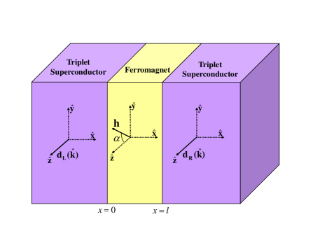
Figure 1: (Color online) Scheme of triplet SFS junction. Here, L,R label the left and right half-spaces. Two superconducting bulks are separated by a ferromagnetic layer with the exchange field $\mathbf{h}$.

In Refs.Kastening ; Brydon1 ; Brydon2 the authors demonstrated presence of both charge and spin currents in the systems consisting of a thin barrier of ferromagnet sandwiched between two triplet superconductors. They obtained a spin current due to the coupling of the ferromagnetic moment to the spin of triplet Cooper pairs. Also, they found a 0-$\pi$ transition in the triplet superconductor-ferromagnet-superconductor (SFS) Josephson junction generated by the misalignment of the $d$-vectors of the triplet superconductors with respect to the magnetic moment of the ferromagnet. In contrast to Refs.Kastening ; Brydon1 ; Brydon2 where the ferromagnet is modeled as $\delta$ function potential, in this paper we allow for arbitrary length of the ferromagnet, which is a more realistic modeling, based on the quasiclassical Eilenberger equation.

In this paper, we investigate a triplet SFS structure with arbitrary misalignment between magnetization of the ferromagnet and gap vector of superconductors (Fig.1), by changing the exchange field and thickness of ferromagnetic layer. We find that charge and spin currents show 0-$\pi$ transition except for the case that the two vectors are in nearly perpendicular configuration

The organization of this paper is as follows. In Sec.II the quasiclassical equations for Green functions are presented. In Sec.III, we calculate Green functions of the system analytically, presenting the formulas for the Green functions to calculate the charge and spin current densities. In Sec.IV, we show the results of spin and charge currents. The paper will be finished with the conclusions in Sec.V.

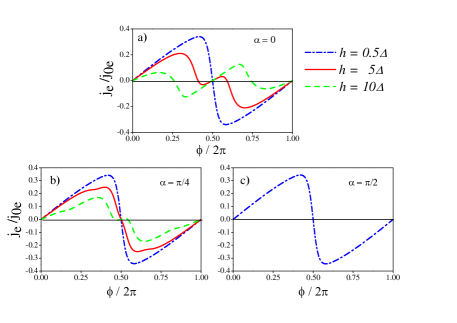
Figure 2: (Color online)The $x$ component of the charge current versus the phase difference $\phi$ for $l=\xi/2$, $T=0.05T_{C}$, and different $h$ and $\alpha$. Currents are given in units of $j_{0,e}=\frac{\pi}{2}eN(0)v_{F}\Delta(0)$.

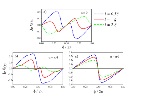
Figure 3: (Color online) The $x$ component of the charge current versus the phase difference $\phi$ for $h=5\Delta$, $T=0.05T_{C}$, and different $l$ and $\alpha$.

II Formalism and Basic equations

We consider a clean SFS structure with a homogenous ferromagnet of thickness $l$ and bulk triplet superconductors(see Fig.1). The ferromagnetic layer is characterized by an exchange field $\mathbf{h}$. There is a misorientation angle $\alpha$ between the exchange field of ferromagnet and order parameters of superconductors ($\mathbf{d}$-vectors). Interfaces are fully transparent and magnetically inactive. The thickness $l$ is larger than the Fermi wave length and smaller than the elastic mean free path. Then, we can use a quasiclassical description in the clean limit, and apply the Eilenberger equation in this limitEilenberger ; Kulik ; Kupriyanov :

$$\mathbf{v}_{F}\nabla\breve{g}+\left[\varepsilon_{m}\breve{\sigma}_{3}+i(\breve{\Delta}+\breve{\mathbf{h}}),\breve{g}\right]=0,$$ (1)

with the normalization condition $\breve{g}\breve{g}=\breve{I}$. Here, $\varepsilon_{m}=\pi T(2m+1)$ are discrete Matsubara energies, $T$ is the temperature, $\mathbf{v}_{F}$ is the Fermi velocity and $\breve{\sigma}_{3}=\hat{\tau}_{3}\otimes\hat{I}$ in which $\hat{\tau}_{3}$ is the third Pauli matrix in particle-hole space. $\hat{\sigma}_{j}\left(j=1,2,3\right)$ denote Pauli matrices in spin space in the following. The Matsubara propagator $\breve{g}$ can be written in the standard form:

$$\breve{g}=\left(\begin{array}[]{cc}g_{1}+\mathbf{g}_{1}\cdot\hat{\bm{\sigma}}&\left(g_{2}+\mathbf{g}_{2}\cdot\hat{\bm{\sigma}}\right)i\hat{\sigma}_{2}\\ i\hat{\sigma}_{2}\left(g_{3}+\mathbf{g}_{3}\cdot\hat{\bm{\sigma}}\right)&g_{4}-\hat{\sigma}_{2}(\mathbf{g}_{4}\cdot\hat{\bm{\sigma}})\hat{\sigma}_{2}\end{array}\right)$$ (2)

where $\hat{\bm{\sigma}}=(\hat{\sigma}_{1},\hat{\sigma}_{2},\hat{\sigma}_{3})$ is the vector of Pauli matrices in spin space. Also, we can write $\breve{\mathbf{h}}$ as follows:

$$\breve{\mathbf{h}}=\left(\begin{array}[]{cc}\mathbf{h}\cdot\hat{\bm{\sigma}}&0\\ 0&(\mathbf{h}\cdot\hat{\bm{\sigma}})^{*}\end{array}\right).$$ (3)

We use Eilenberger equation for both ferromagnetic and superconducting materials. For superconductors we set $\mathbf{h}=0$. The matrix structure of the off-diagonal self energy $\breve{\Delta}$ in the Nambu space is

$$\breve{\Delta}=\left(\begin{array}[]{cc}0&(\mathbf{d}\cdot\hat{\bm{\sigma}})i\hat{\sigma}_{2}\\ i\hat{\sigma}_{2}(\mathbf{{d^{\ast}}\cdot\hat{\bm{\sigma}})}&0\end{array}\right).$$ (4)

In the ferromagnet we set $\breve{\Delta}=0$ and $\mathbf{h}=(0,h\sin\alpha,h\cos\alpha)$. In this paper, the unitary state, $\mathbf{d\times d}^{\ast}=0,$ is investigated.

Solutions of Eq. (1) have to satisfy the conditions for Green functions in the bulks of the superconductors:

$$\breve{g}\left(\pm\infty\right)=\frac{\varepsilon_{m}\breve{\sigma}_{3}+i\breve{\Delta}_{1,2}}{\sqrt{\varepsilon_{m}^{2}+\left|\mathbf{d}_{1,2}\right|^{2}}},$$ (5)

$$\mathbf{d}_{1,2}=\mathbf{d}_{L,R}\left(\mathbf{\hat{v}}_{F}\right)\exp\left(\pm\frac{i\phi}{2}\right),$$ (6)

where $\phi$ is the external phase difference between the order parameters of the bulks of superconductors. Eq. (1) have to be supplemented by the continuity conditions at the interfaces between ferromagnet and superconductors. For all quasiparticle trajectories, the Green functions satisfy the boundary conditions both in the right and left bulks as well as at the interfaces.

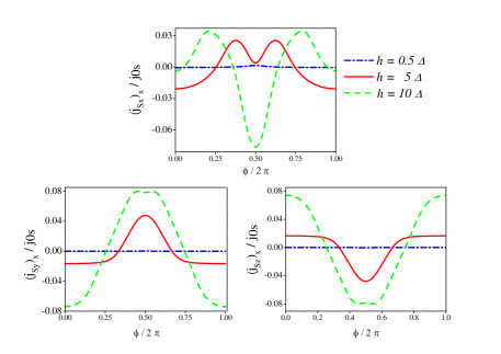
Figure 4: (Color online) The normal component ($x$ component) of the spin current at the left interface, versus the phase difference $\phi$, for $l=\xi/2$, $T=0.05T_{C}$, different $h$ and $\alpha=\pi/4$. Currents are calculated in units of $j_{0,s}=\frac{\pi}{2}\hbar N(0)v_{F}\Delta(0)$.

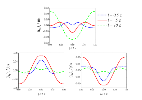
Figure 5: (Color online) The $x$ component of the spin current at the left interface, versus the phase difference $\phi$ for $h=5\Delta$, $T=0.05T_{C}$, $\alpha=\pi/4$ and different $l$.

III analytical Results of Green functions

In principle, Eilenberger equations (1) should be supplemented with a self-consistent equation for gap vector. While these numerical self-consistent calculations can be used to investigate the spatial variation of gap vector in the superconductors and also the dependence of gap vector on temperature, in this paper we do not apply them. In our analytical calculations, we consider a step-like function of gap vector which is zero in the ferromagnet and finite value in the superconducting part. It has been shown that the absolute value of a self-consistently detemined order parameter decreases near the interface between superconductor and normal metal, while its dependence on the direction of Fermi velocity remains unalteredBarash . In Refs.Coury ; Barash ; Thuneberg ; Viljas a qualitative agreement between self-consistent and non-self-consistent calculations for unconventional Josephson junctions is found. Also, it is observed that the results of non-self-consistent calculation in Ref.Faraii are coincident with the experimental data in Ref.Freamat . Also, the results by non-self-consistent treatment in Ref.Yip are similar to the experimental results in Ref. Backhaus . Consequently, we believe that non-self-consistent approximation doesn’t change results qualitatively. Therefore, in our calculations, a simple model of the constant order parameter up to the interface is considered to obtain qualitative results. Using such a model, the analytical expressions for the charge and spin currents in the ferromagnet and superconductors can be obtained for a specified form of the order parameter. The expressions for the charge and spin currents are the followings:Serene ; Viljas

$$\mathbf{j}_{e}\left(\mathbf{r}\right)=2i\pi eTN\left(0\right)\sum_{m}\left\langle\mathbf{v}_{F}g_{1}\left(\mathbf{\hat{v}}_{F},\mathbf{r},\varepsilon_{m}\right)\right\rangle,$$ (7)

$$\mathbf{j}_{s_{i}}\left(\mathbf{r}\right)=\pi\hbar TN\left(0\right)\sum_{m}\left\langle\mathbf{v}_{F}\left(\mathbf{{\hat{e}}}_{i}\cdot\mathbf{g}_{1}\left(\mathbf{\hat{v}}_{F},\mathbf{r},\varepsilon_{m}\right)\right)\right\rangle$$ (8)

where $\mathbf{{\hat{e}}}_{i}\mathbf{=}\left(\hat{\mathbf{x}},\hat{\mathbf{y}},\hat{\mathbf{z}}\right)$ and $N(0)$ is the density of states in the normal state at the Fermi energy. We consider the order parameter as follows:

$$\mathbf{d}_{n}(T,\mathbf{\hat{v}}_{F},\mathbf{r})=d_{n}(T,\mathbf{\hat{v}}_{F},\mathbf{r})\hat{\mathbf{z}}.$$ (9)

Solving Eilenberger equation in ferromagnet region and superconductors under the continuity of solutions across the interfaces, $x=0,l$ and the boundary conditions at the bulks, we obtain the Green’s functions in the ferromagnet region. The Green’s functions are given by

$$g_{1F}=\frac{\eta(p^{2}-1)\left(p^{2}+2p[\beta+\sin^{2}\alpha(2\beta^{2}-\beta-1)]+1\right)}{D},$$ (10)

and

$$\mathbf{g}_{1F}=\frac{\eta p}{D}\left(\begin{array}[]{cc}A\cos(\frac{2hx}{v_{x}})+B\sin(\frac{2hx}{v_{x}})\\ \cos\alpha[A\sin(\frac{2hx}{v_{x}})-B\cos(\frac{2hx}{v_{x}})]+C\sin\alpha\\ \sin\alpha[B\cos(\frac{2hx}{v_{x}})-A\sin(\frac{2hx}{v_{x}})]+C\cos\alpha\end{array}\right)$$ (14)

where

$$A = \sin 2\alpha[\beta-1][p^{2}(2\beta+1)+2p(\beta\sin^{2}\alpha+\cos^{2}\alpha)-1],$$

$$B = \sin 2\alpha\sin(2hl/v_{x})[p^{2}(2\beta-1)+2p(\beta\sin^{2}\alpha+\cos^{2}\alpha)+1],$$

$$C = 2\cos^{2}\alpha\sin(2hl/v_{x})[p^{2}+2p\left(\sin^{2}\alpha(\beta-1)+\beta\right)+1],$$

$$D = p^{4}+2p^{2}[2(\beta\sin^{2}\alpha+\cos^{2}\alpha)^{2}+2\beta^{2}-1]+4p\beta(p^{2}+1)(\beta\sin^{2}\alpha+\cos^{2}\alpha)+1,$$

$$\beta = \cos(2hl/v_{x})$$

$$\eta = sgn\left(v_{x}\right)$$

$$p = \frac{d_{1}d_{2}^{*}\exp(-2\varepsilon_{m}l/v_{x})}{(\varepsilon_{m}+\eta\Omega_{1})(\varepsilon_{m}+\eta\Omega_{2})}$$

$$\Omega_{1,2} = \sqrt{\varepsilon_{m}^{2}+\left|\mathbf{d}_{1,2}\right|^{2}}.$$

For parallel alignment of gap vector and exchange field, $\alpha=0$, Green’s functions reduce to

$$g_{1F} = \frac{\eta(p^{2}-1)}{p^{2}+2p\beta+1},$$

$$\mathbf{g}_{1F} = \frac{2\eta p\sin(2hl/v_{x})}{p^{2}+2p\beta+1}\mathbf{\hat{z}}.$$ (15)

It is seen from this expression that Green’s functions and hence charge and spin currents depend on the exchange field through $\beta$. Also, for the perpendicular configuration $\alpha=\frac{\pi}{2}$, we obtain

$$g_{1F} = \frac{\eta(p-1)}{p+1},$$

$$\mathbf{g}_{1F} = 0$$ (16)

where the Green’s function are independent of the exchange field. As a result, we do not see any $0-\pi$ transition in this casePowell .

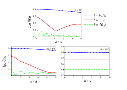
Figure 6: (Color online) The $x$ component of the critical charge current versus $h$ for $T=0.05T_{C}$ and different $l$ and different $\alpha$

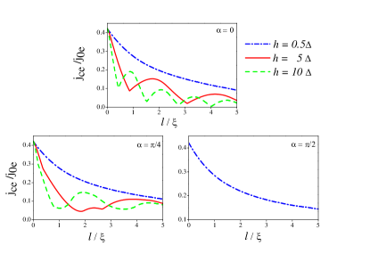
Figure 7: (Color online) The $x$ component of the critical charge current versus the thickness of the ferromagnetic layer at $T=0.05T_{C}$ for different $h$ and different $\alpha$

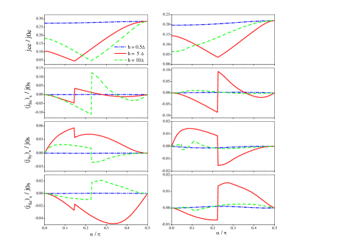
Figure 8: (Color online) The $x$ component of the critical charge and spin currents versus $\alpha$ for $T=0.05T_{C}$. Left panels are for $l=\xi$ and right panels are for $l=2\xi$.

IV Numerical Results of Charge and Spin Currents

Here, we have considered $p-$wave superconductors with the model of order parameter as

$$d(T,\mathbf{\hat{v}}_{F},\mathbf{r})=\Delta(T)\left(k_{x}+ik_{y}\right)$$ (17)

which would be realized in Sr₂RuO₄Mackenzie . The function $\Delta\left(T\right)$ describes the dependence of the order parameter $\mathbf{d}$ on the temperature $T$. We have used Green functions in Eqs.(10) and (14) and calculated charge and spin currents for our specified model of the order parameter. For representative values of $h$, $l$ and $\alpha$, we have shown charge and spin currents in Figs. 2-5 as a function of phase difference between superconductors. In the figures, $\xi(T)=\frac{\hbar v_{F}}{\pi\Delta(T)}$ denotes a superconductor coherence length at the bulk of superconductor. By changing the parameters, we find a tendency towards the 0-$\pi$ transition. In particular, we see a stronger tendency towards the 0-$\pi$ transition at $\alpha=0$.

In our formalism, there are in general three components ($s_{x}$, $s_{y}$ and $s_{z}$) of spin current due to the presence of the ferromagnetic layer with finite thickness. While charge current is independent of position in ferromagnet, spin current is dependent on position and is not conserved. In fact, spin current at the left and right interfaces have opposite sign and in the middle of ferromagnetic layer, the spin current vanishes. We have plotted spin current at the left interface between superconductor and ferromagnetic layer in Figs. 4,5 and Fig.8. At this point, there are three components of spin current.

For charge current, we see that by increasing the thickness of ferromagnetic layer the current decreases with oscillation because of decreasing of quantum coherency, but for the spin current the situation is quite different. As a result of the exchange field, the thicker layer has a greater effect on spin of quasiparticles and thus a larger spin current. As seen in Fig.2 for $\alpha=\pi/2$, the results are independent of the exchange field. Thus, charge current in this case is only dependent on thickness of the ferromagnetic layer and spin current is absent. Regarding spin currents, all components of spin current vanish at $\alpha=0$ and $\alpha=\pi/2$. As shown in Fig.4, spin current is strongly dependent on the exchange field, so for a weak ferromagnet (for example $h=0.5\Delta$), spin current is negligibly small. For some values of the phase difference, spin current exists in the absence of charge current as seen from Figs. 4 and 5. Also, there is local maximum or minimum in spin current in $\phi=0$ or $\phi=\pi$. This can be explained as follows. Charge currents are generally odd function but spin currents are even function of the phase difference, because of the symmetry under the time reversal. Therefore, the slope of the spin current becomes zero at $\phi=0$ and $\phi=\pi$.

The critical currents as a function of $h$ and $l$ are shown in Fig.6 and Fig.7 for different misorientations $\alpha=0$, $\pi/4$ and $\pi/2$. Also, critical charge and spin currents as the function of $\alpha$ have been plotted in Fig.8. Here, the critical charge and spin currents are defined as $j_{ce}=Max_{\phi}j_{e}(\phi)=j_{e}(\phi^{\ast})$ and $j_{s}=j_{s}(\phi^{\ast})$, respectively. The 0-$\pi$ transition as a function of $h$ for large $l$ and small $\alpha$ are shown in Fig.6. In Ref.Brydon2 , it is shown that 0-$\pi$ transition cannot occur at $\alpha=\pi/2$ for a $\delta$ function type ferromagnetic barrier. We find that this is the case even in the presence of a ferromagnetic layer with finite thickness instead of a $\delta$ function type barrier. This is also seen from the dependence of the Josephson current on $l$ which shows the 0-$\pi$ transition for large $h$ and small $\alpha$ as seen in Fig.7. As shown in Fig.8, for finite thickness of ferromagnetic layer, 0-$\pi$ transition can be found with changing the misorinetation angle. The 0-$\pi$ transition is accompanied by the jump of the spin current due to the phase jump at the 0-$\pi$ transition.Alidoust Even when charge current shows a monotonous dependence on $\alpha$, spin current can show non-monotonous $\alpha$ dependence.

V Conclusions

In this paper, we have investigated transport properties in triplet SFS Josephson junction and clarified the effects of the thickness of ferromagnet, the exchange field, and misorientation angle between exchange field of ferromagnet and $d$-vector of superconductors on the Josephson charge and spin currents. We found that 0-$\pi$ transition can occur except for the case that the exchange field and d-vector are in nearly perpendicular configuration. Also, we showed how spin current flows due to misorientation between the exchange field and $d$-vector and found that it is absent when two vectors are parallel or perpendicular to each other.

VI Acknowledgement

We would like to thank J. Linder and P. M. R. Brydon for their helpful discussions and their comments on draft of our paper.

References

- (1) A. I. Buzdin, Rev. Mod. Phys. 77, 935 (2005).
- (2) F. S. Bergeret, A. F. Volkov, and K. B. Efetov, Rev. Mod. Phys. 77, 1321 (2005).
- (3) A. F. Volkov, and K. B. Efetov, Phys. Rev. B. 78, 024519 (2008).
- (4) M. Zareyan, W. Belzig, and Yu. V. Nazarov, Phys. Rev. B. 65, 184505 (2002).
- (5) V. Braude and Ya. M. Blanter, Phys. Rev. Lett. 100, 207001 (2008).
- (6) F. S. Bergeret, A. F. Volkov, and K. B. Efetov, Phys. Rev. Lett. 86, 4096 (2001); A. F. Volkov, F. S. Bergeret, and K. B. Efetov, Phys. Rev. Lett. 90, 117006 (2003).
- (7) A. Kadigrobov, R. I. Shekter and M. Jonson, Europhys. Lett. 90, 394 (2001).
- (8) M. Eschrig, T. Löfwander, Th. Champel, J. C. Cuevas, and G. Scḧon, J. Low Temp. Phys. 147 457 (2007).
- (9) M. Eschrig and T. Löfwander, Nature Physics 4, 138 (2008).
- (10) T. Yokoyama, Y. Tanaka, and A. A. Golubov, Phys. Rev. B 75, 134510 (2007);T. Yokoyama and Y. Tserkovnyak, Phys. Rev. B 80, 104416 (2009).
- (11) J. Linder, T. Yokoyama, A. Sudbø, and M. Eschrig, Phys. Rev. Lett. 102, 107008 (2009); J. Linder, T. Yokoyama, and A. Sudbø, Phys. Rev. B 79, 054523 (2009);J. Linder, A. Sudbo, T. Yokoyama, R. Grein and M. Eschrig, Phys. Rev. B 81, 214504 (2010).
- (12) M. Alidoust, J. Linder, G. Rashedi, T. Yokoyama, and A. Sudbo Phys. Rev. B. 81, 014512 (2010).
- (13) Y. Maeno, H. Hashimoto, K. Yoshida, S. Nishizaki, T. Fujita, J. G. Bednorz, and F. Lichtenberg, Nature (London) 372, 532 (1994).
- (14) K. Ishida, H. Mukuda, Y. Kitaoka, K. Asayama, Z. Q. Mao, Y. Mori, and Y. Maeno, Nature (London) 396, 658 (1998).
- (15) G. M. Luke, Y. Fudamoto, K. M. Kojima, M. I. Larkin, J. Merrin, B. Nachumi, Y. J. Uemura, Y. Maeno, Z. Q. Mao, Y. Mori, H. Nakamura, and M. Sigrist, Nature (London) 394, 558 (1998).
- (16) A. P. Mackenzie and Y. Maeno, Rev. Mod. Phys. 75, 657 (2003).
- (17) K. D. Nelson, Z. Q. Mao, Y. Maeno and Y. Liu, Science 306, 1151 (2004).
- (18) Y. Asano, Y. Tanaka, M. Sigrist and S. Kashiwaya, Phys. Rev. B 67, 184505 (2003); Phys. Rev. B 71, 214501 (2005).
- (19) H. Tou, Y. Kitaoka, K. Ishida, K. Asayama, N. Kimura, Y. Onuki, E. Yamamoto, Y. Haga and K. Maezawa, Phys. Rev. Lett. 80, 3129 (1998).
- (20) V. Muller, Ch. Roth, D. Maurer, E. W. Scheidt, K. Lers, E. Bucher and H. E. Bmel, Phys. Rev. Lett. 58, 1224 (1987).
- (21) Y. J. Qian, M. F. Xu, A. Schenstrom, H. P. Baum, J. B. Ketterson, D. Hinks, M. Levy and B. K. Sarma, Solid State Commun., 63, 599 (1987).
- (22) A. A. Abrikosov, J. of Low Temp. Phys. 53, 359 (1983).
- (23) H. Fukuyama and Y. Hasegawa, J. Phys. Soc. Jpn 56, 877 (1987).
- (24) A. G. Lebed, K. Machida and M. Ozaki, Phys. Rev. B 62, 795 (2000).
- (25) S. S. Saxena, P. Agarwal, K. Ahilan, F. M. Grosche, R. K. W. Haselwimmer, M. J. Steiner, E. Pugh, I. R. Walker, S. R. Julian, P. Monthoux, G. G. Lonzarich, A. Huxley, I. Shelkin, D. Braithwaite, and J. Flouquet, Nature (London) 406, 587 (2000).
- (26) C. Pfleiderer, M. Uhlarz, S. M. Hayden, R. Vollmer, H. v. Lohneysen, N. R. Bernhoeft, and G. G. Lonzarich, Nature (London) 412, 58 (2001).
- (27) D. Aoki, A. Huxley, E. Ressouche, D. Braithwaite, J. Flouquet, J. Brison, E. Lhotel, and C. Paulsen, Nature (London) 413, 613 (2001).
- (28) C. J. Bolech and T. Giamarchi, Phys. Rev. Lett. 92, 127001 (2004); Phys. Rev. B 71, 024517 (2005).
- (29) M. S. Grønsleth, J. Linder, J.-M. Børven, and A. Sudbø, Phys. Rev. Lett. 97, 147002 (2006); Phys. Rev. B 75, 054518 (2007).
- (30) Y. Asano, Phys. Rev. B 72, 092508 (2005); Phys. Rev. B 74, 220501(R) (2006).
- (31) R. Mahmoodi, Yu. A. Kolesnichenko and S. N. Shevchenko, Fiz. Nizk. Temp. 28 262 (2002) [Low Temp. Phys. 28 184 (2002)].
- (32) G. Rashedi and Yu A. Kolesnichenko, Physica C, 451 31 (2007); G. Rashedi and Yu A. Kolesnichenko, Supercond. Sci. Technol. 18, 482 (2005).
- (33) G. Rashedi, Y. Rahnavard, Yu. A. Kolesnichenko, Fiz. Nizk. Temp. 36 262 (2010) [Low Temp. Phys. 36, 205 (2010)].
- (34) G. Rashedi and Yu. A. Kolesnichenko, Fiz. Nizk. Temp. 31 634 (2005) [Low Temp. Phys. 31, 481 (2005)]
- (35) Y. Rahnavard, G. Rashedi and T. Yokoyama, J. Phys. Condens. Matter 22, 415701(2010) .
- (36) B. Kastening, D. K. Morr, D. Manske, and K. Bennemann, Phys. Rev. Lett. 96, 047009 (2006).
- (37) P. M. R. Brydon, B. Kastening, D. K. Morr, and D. Manske, Phys. Rev. B. 77, 104504 (2008).
- (38) P. M. R. Brydon and D. Manske, Phys. Rev. Lett. 103, 147001 (2009); P. M. R. Brydon, C Iniotakis, and Dirk Manske, New Journal of Physics 11, 055055 (2009).
- (39) G. Eilenberger, Z. Phys. 214, 195 (1968).
- (40) I. O. Kulik, and A. N. Omelyanchuk,, Fiz. Nizk. Temp. 4, 296 (1978)[Sov. J. Low Temp. Phys. 4, 142 (1978)].
- (41) M. Yu. Kupriyanov, Fiz. Nizk. Temp. 7, 700 (1981)[Sov. J. Low. Temp. Phys. 7, 342 (1981)].
- (42) Yu. S. Barash, A.M. Bobkov, and M. Fogelström, Phys. Rev. B 64, 214503 (2001).
- (43) M.H.S. Amin, M.Coury, S.N. Rashkeev, A.N. Omelyanchouk, and A.M. Zagoskin, Physica B, 318, 162 (2002).
- (44) J.K. Viljas, E.V. Thuneberg, Phys. Rev. B 65, 64530 (2002).
- (45) J. Viljas, cond-mat/0004246.
- (46) Z. Faraii and M. Zareyan, Phys. Rev. B 69, 014508(2004).
- (47) M. Freamat, K.-W. Ng, Phys. Rev. B 68, 060507 (2003).
- (48) S.-K. Yip, Phys. Rev. Lett. 83, 3864 (1999).
- (49) S. Backhaus, S. Pereverzev, R.W. Simmonds, A. Loshak, J.C. Davis, and R.E. Packard, Nature 392, 687 (1998).
- (50) J. Serene and D. Rainer, Phys. Reports 101, 221 (1983).
- (51) B. J. Powell, J. F. Annett and B. L. Györffy, J. Phys. A: Math. Gen. 36 9289 (2003).