Binary Independent Component Analysis with OR Mixtures

Abstract

Independent component analysis (ICA) is a computational method for separating a multivariate signal into subcomponents assuming the mutual statistical independence of the non-Gaussian source signals. The classical Independent Components Analysis (ICA) framework usually assumes linear combinations of independent sources over the field of real-valued numbers $\mathcal{R}$. In this paper, we investigate binary ICA for OR mixtures (bICA), which can find applications in many domains including medical diagnosis, multi-cluster assignment, Internet tomography and network resource management. We prove that bICA is uniquely identifiable under the disjunctive generation model, and propose a deterministic iterative algorithm to determine the distribution of the latent random variables and the mixing matrix. The inverse problem concerning inferring the values of latent variables are also considered along with noisy measurements. We conduct an extensive simulation study to verify the effectiveness of the propose algorithm and present examples of real-world applications where bICA can be applied.

I Introduction

Independent component analysis (ICA) is a computational method for separating a multivariate signal into additive subcomponents supposing the mutual statistical independence of the non-Gaussian source signals. The classical Independent Components Analysis (ICA) framework usually assumes linear combinations of independent sources over the field of real-valued numbers $\mathcal{R}$. Consider the following generative data model where the observations are disjunctive mixtures of binary independent sources. Let $\mbox{$\mathbf{x}$}=[x_{1},x_{2},\ldots,x_{n}]^{T}$ be a $m$-dimension binary random vector with joint distribution $\mathcal{P}(\mbox{$\mathbf{x}$})$, which are observable. $\mathbf{x}$ is generated from a set of $n$ independent binary random variables $\mbox{$\mathbf{y}$}=[y_{1},y_{2},\ldots,y_{n}]^{T}$ as follows,

$$x_{i}=\bigvee_{j=1}^{n}{(g_{ij}\wedge y_{j})},\mbox{ $i=1,\ldots,m$},$$ (1)

where $\wedge$ is Boolean AND, $\vee$ is Boolean OR, and $g_{ij}$ is the entry in the $i$’th row and $j$’th column of an unknown binary mixing matrix $G$. Throughout this paper, we denote by $\mbox{\boldmath$G$}_{i,:}$ and $\mbox{\boldmath$G$}_{:,j}$ the $i$’th row and $j$’th column of matrix $G$ respectively. For the ease of presentation, we introduce a short-hand notation for the above disjunctive model as,

$$\mbox{$\mathbf{x}$}=\mbox{\boldmath$G$}\otimes\mbox{$\mathbf{y}$}.$$

The relationship between observable variables in $\mathbf{x}$ and latent binary variables in $\mathbf{y}$ can also be represented by an undirected bi-partite graph $G=(U,V,E)$, where $U=\{x_{1},x_{2},\ldots,x_{m}\}$ and $V=\{y_{1},y_{2},\ldots,y_{n}\}$ (Figure 1). An edge $e=(x_{i},y_{j})$ exists if $g_{ij}=1$. We will refer to $G$ as the binary adjacency matrix of graph $G$. The key notations used in this paper are listed in Table I.

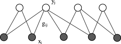
Figure 1: Illustration of the OR mixture model

Consider an $m\times T$ matrix $X$ and an $n\times T$ matrix $Y$, which are the collection of $T$ realizations of random vector $\mathbf{x}$ and $\mathbf{y}$ respectively. The goal of binary independent component analysis with OR mixtures (bICA) is to estimate the distribution of the latency random variables $\mathbf{y}$ and the binary mixing matrix $G$ from $X$ such that $X$ can be decomposed into OR mixtures of columns of $Y$.

In this paper, we make the following contributions. First, we investigate the identifiability of bICA and prove that under the disjunctive generation model, the OR mixing is identifiable up to permutation. Second, we develop an iterative algorithm for bICA that does not make assumptions on the noise model or prior distributions of the mixing matrix. Interestingly, the approach is shown to be robust under moderate to medium XOR noises and insufficient samples. We furthermore consider the inverse problem of inferring the values of $\mathbf{y}$ given noisy observations $X$ and the inferred model. Finally, we present two case studies to illustrate how bICA can be used to model and solve real-world problems. .

TABLE I: Notations

	the number of observable variables,
$m,n,T$	hidden variables and observations
	the bi-partite graph representing the
$G$	observable-hidden variable relationship
	the vector of $m$ binary observations
$\mbox{$\mathbf{x}$}_{m\times 1}$	from $m$ observable variables
	the vector of $n$ binary activities
$\mbox{$\mathbf{y}$}_{n\times 1}$	from $n$ hidden variables
	the collection of $T$ realizations of $\mathbf{x}$
$\mbox{\boldmath$X$}_{m\times T}$	(observation matrix)
	the collection of $T$ realizations of $\mathbf{y}$
$\mbox{\boldmath$Y$}_{n\times T}$	(activity matrix)
$\mbox{\boldmath$G$}_{m\times n}$	the binary adjacency matrix of graph $G$
	the probability vector associated with
$p_{1\times n}$	$n$ (Bernoulli) hidden variables

The rest of the paper is organized as follows. In Section II, we give a brief overview of related work. In Section III, several important properties of bICA are proved. In Section IV, we elaborate on an iterative procedure to infer bICA and several complexity reduction techniques. Formulation and solution to the inverse problem with noisy measurements are presented in Section V. Effectiveness of the proposed method is evaluated through simulation results in Section VI. Real-world problem domains where bICA can be applied are discussed in Section VII and followed by conclusion and future work in Section VIII.

II Related work

Most ICA methods assume linear mixing of continuous signals [1]. A special variant of ICA, called binary ICA (BICA), considers boolean mixing (e.g., OR, XOR etc.) of binary signals. Existing solutions to BICA mainly differ in their assumptions of the binary operator (e.g., OR or XOR), the prior distribution of the mixing matrix, noise model, and/or hidden causes.

In [2], Yeredor considers BICA in XOR mixtures and investigates the identifiability problem. A deflation algorithm is proposed for source separation based on entropy minimization. Since XOR is addition in GF(2), BICA in XOR mixtures can be viewed as the binary counterpart of classical linear ICA problems. In [2], the number of independent random sources $K$ is assumed to be known. Furthermore, the mixing matrix is a $K$-by-$K$ invertible matrix. Under these constraints, it has been proved that the XOR model is invertible and there exist a unique transformation matrix to recover the independent components up to permutation ambiguity. Though our proof of identifiability in this paper is inspired by the approach in [2], due to the “non-linearity” of OR operations, the notion of invertible matrices no longer apply. New proofs and algorithms are warranted to unravel the properties of binary OR mixtures.

In [3], the problem of factorization and de-noise of binary data due to independent continuous sources is considered. The sources are assumed to be continuous following beta distribution in [0, 1]. Conditional on the latent variables, the observations follow the independent Bernoulli likelihood model with mean vectors taking the form of a linear mixture of the latent variables. The mixing coefficients are assumed to non-negative and sum to one. A variational EM solution is devised to infer the mixing coefficients. A post-process step is applied to quantize the recovered “gray-scale” sources into binary ones. While the mixing model in [3] can find many real world applications, it is not suitable in the case of OR mixtures.

In [4], a noise-OR model is introduced to model dependency among observable random variables using $K$ (known) latent factors. A variational inference algorithm is developed. In the noise-OR model, the probabilistic dependency between observable vectors and latent vectors is modeled via the noise-OR conditional distribution. The dimension of the latent vector is assumed to be known and less than that of the observable.

In [5], Wood et al. consider the problem of inferring infinite number of hidden causes following the same Bernoulli distribution. Observations are generated from a noise-OR distribution. Prior of the infinite mixing matrix is modeled as the Indian buffet process [6]. Reversible jump Markov chain Monte Carlo and Gibbs sampler techniques are applied to determine the mixing matrix based on observations. In our model, the hidden causes are finite in size, and may follow different distribution. Streith et al. [7] study the problem of multi-assignment clustering for boolean data, where the observations are either drawn from a signal following OR mixtures or from a noise component. The key assumption made in the work is that the elements of matrix $X$ are conditionally independent given the model parameters (as opposed to the latent variables). This greatly reduces the computational complexity and makes the scheme amenable to a gradient descent-based optimization solution. However, this assumption is in general invalid.

There exists a large body of work on blind deconvolution with binary sources in the context of wireless communication [8, 9]. In time-invariant linear channels, the output signal $x(k)$ is a convolution of the channel realizations $a(k)$ and the input signal $s(k)$, $k=1,2,\ldots,K$ as follows:

$$x(k)=\sum_{l=0}^{L}{a(l)s(k-l)},k=1,\ldots,K.$$ (2)

The objective is to recover the input signal $s$. Both stochastic and deterministic approaches have been devised for blind deconvolution. As evident from (2), the output signals are linear mixtures of the input sources in time, and additionally the mixture model follows a specific structure.

Algorithm	Sources	Generative model	Under/Over determined	Dimension of latent variables
[2]	Binary	Binary XOR	–	Known
[3]	Continuous	Linear	Over	Known
[4]	Binary	Noise-OR	Over	Known
[5]	Binary	Noise-OR	Under	Infinite
[7]	Binary	Binary OR	Over	Known
[10, 11]	Binary	Binary OR	Over	Unknown, try to minimize
[8, 9]	Binary	Linear	–	Known
bICA	Binary	Binary OR	Under	Unknown but finite

TABLE II: Related work comparison chart

Literature on boolean/binary factor analysis (BFA) is also related to our work. The goal of BFA is to decompose a binary matrix $\mbox{\boldmath$X$}_{m\times T}$ into $\mbox{\boldmath$A$}_{m\times n}\otimes\mbox{\boldmath$B$}_{n\times T}$ with $\otimes$ being the OR mixture relationship as defined in (1). $X$ in BFA is often called an attribute-object matrix providing $m$-dimension attributes of $T$ objects. $A$ and $B$ are the attribute-factor and factor-object matrices. All the elements in $X$, $A$, and $B$ are either 0 or 1. $n$ is defined to be the number of underlying factors and is assumed to be considerably smaller than the number of objects $T$. BFA methods aim to find a feasible decomposition minimizing $n$. Frolov et al. study the problem of factoring a binary matrix using Hopfield neural networks [12, 10, 13]. This approach is based on heuristic and do not provide much theoretical insight regarding the properties of the resulting decomposition. More recently, Belohlavek et al. propose a matrix decomposition method utilizing formal concept analysis [11]. The paper claims that optimal decomposition with the minimum number of factors are those where factors are formal concepts. It is important to note that even though BFA assumes the same disjunctive mixture model as in our work, the objective is different. While BFA tries to find a matrix factorization so that the number of factors are minimized, bICA tries to identify independent components. One can easily come up an example, where the number of independent components (factors) is larger than the number of attributes. Since BFA always finds factors no larger than the number of attributes, the resulting factors are clearly dependent in this case.

Finally, [5] consider the under-presented case of less observations than latent sources with continuous noise, while [3, 7, 10, 11] deal with the over-determined case, where the number of observation variables are much larger. In this work, we consider primarily the under-presented cases that we typically encounter in data networks where the number of sensors are much smaller and the number of signal sources (i.e. users).

We summarize the aforementioned related work in Table II.

III Properties of bICA

In this section, we investigate the fundamental properties of bICA. In particular, we are interested in the following questions:

• Expressiveness: can any set of binary random variables be decomposed into binary independent components using OR mixtures?

• Independence of OR mixtures: for mixtures of independent sources, what is the condition that they are independent?

• Identifiability: given a set of binary random variables following the bICA data model, is the decomposition unique?

Expressiveness

Expressiveness of OR mixtures is limited. This can be shown through an example. Let $y_{1}$ and $y_{2}$ be two independent binary random variables with $P(y_{1}=1)=p\neq 0.5$ and $P(y_{2}=1)=q\neq 0.5$. Let $x_{1}=y_{1}$ and $x_{2}=y_{1}+y_{2}$, where ‘+’ is addition in the finite field GF(2). It is easy to see that $x_{1}$ and $x_{2}$ are correlated since $P(x_{2}=1)=P(y_{1}=1)P(y_{2}=0)+P(y_{1}=0)P(y_{2}=1)=q(1-p)+p(1-q)$, $P(x_{1}=1)=p$, while $P(x_{1}=1,x_{2}=1)=P(y_{2}=0)=1-q$. On the other hand, $x_{2}$ can not be decomposed into an OR mixture of $y_{1}$ and $y_{2}$. This essentially shows that OR mixtures of binary random variables only span a subset of multi-variate binary distributions. There exist correlated binary random variables ($x_{1},x_{2}$ in this example) that cannot be modeled as OR mixtures of independent binary components.

Independence of mixtures

Now we turn to the second question, namely, under what condition are binary random variables that follow the OR mixture model independent. In general, pairwise independent random variables are not jointly independent. Interestingly, we show that pairwise independence implies joint independence for OR mixtures.

Theorem 1

Let $\mbox{$\mathbf{y}$}=[y_{1},y_{2},\ldots,y_{n}]^{T}$ denote $n$ statistically independent sources in $GF(2)$, the $i$-th source having 1-probability $p_{i}$ . Let $\mbox{$\mathbf{x}$}=\mbox{\boldmath$D$}\otimes\mbox{$\mathbf{y}$}$, where $D$ is a $m\times n$ matrix (with elements in GF(2)). Let $\eta(\mbox{$\mathbf{x}$})$ and $\mbox{\boldmath$C$}(\mbox{$\mathbf{x}$})$ denote the mean and covariance (resp.) of $\mathbf{x}$. If:

1. All elements of $\eta(\mbox{$\mathbf{x}$})$ are nonzero and not 1’s (called non-degenerate),

2. $\mbox{\boldmath$C$}(\mbox{$\mathbf{x}$})$ is diagonal,

Then i) $m=n$, and ii) $D$ is a permutation matrix.

Let us first establish the following lemmas.

Lemma 1

Let $u$ and $v$ be two RVs in GF(2) with 1-probabilities $p_{u}$ and $p_{v}$ (resp.), and let $w\stackrel{{\scriptstyle\Delta}}{{=}}u\vee v$ If $u$ and $v$ are independent, non-degenerate ($0<p,q<1$) then $w$ is also non-degenerate.

Proof:

Clearly, $p_{w}=P(w=1)=1-(1-p_{u})(1-p_{v})$. Since $0<p_{u},p_{v}<1$, we have $0<p_{w}<1$. ∎

Lemma 2

Consider non-degenerate independent binary random variables $y_{1},y_{2},y_{3}$. Then, $x_{1}=y_{1}\vee y_{2}$ and $x_{2}=y_{3}$ are independent.

Proof:

To prove independence of two binary random variables $x_{1}$ and $x_{2}$, it is sufficient to show $P(x_{1}=1,x_{2}=1)=P(x_{1}=1)P(x_{2}=1)$.

$$\begin{array}[]{lll}P(x_{1}=1,x_{2}=1)&=&P(y_{1}=1,y_{2}=1,y_{3}=1)\\ &+&P(y_{1}=1,y_{2}=0,y_{3}=1)\\ &+&P(y_{1}=0,y_{2}=1,y_{3}=1)\\ &=&P(y_{1}=1)P(y_{2}=1)P(y_{3}=1)\\ &+&P(y_{1}=1)P(y_{2}=0)P(y_{3}=1)\\ &+&P(y_{1}=0)P(y_{2}=1)P(y_{3}=1)\\ &=&P(x_{1}=1)P(x_{2}=1)\end{array}$$ (3)

∎

Similar, we can show the following result.

Lemma 3

Consider non-degenerate independent binary random variables $y_{1},y_{2},y_{3}$. Then, $x_{1}=y_{1}\vee y_{2}$ and $x_{2}=y_{1}\vee y_{3}$ are correlated.

Now we are in the position to prove Theorem 1.

Proof:

We prove by contradiction. The essence of the proof is similar to that in [2]. Let us assume now that $D$ is a general matrix, and consider any pair $x_{k}$ and $x_{l}$ ($k\neq l$) in $\mathbf{x}$. $x_{k}$ and $x_{l}$ are OR mixtures of respective subgroups of the sources, indexed by the 1-s in $\mbox{\boldmath$D$}_{k,:}$, and $\mbox{\boldmath$D$}_{l,:}$, the $k$-th and $l$-th rows (respectively) of $D$. These two subgroups consist of, in turn, three other subgroups (some of which may be empty):

1. Sub-group 1: Sources common to $\mbox{\boldmath$D$}_{k,:}$ and $\mbox{\boldmath$D$}_{l,:}$ . Denote the OR mixing of these sources as $u$;

2. Sub-group 2: Sources included in $\mbox{\boldmath$D$}_{k,:}$ but excluded from $\mbox{\boldmath$D$}_{l,:}$. Denote the OR mixing of these sources as $v_{1}$;

3. Sub-group 3: Sources included in $\mbox{\boldmath$D$}_{l,:}$ but excluded from $\mbox{\boldmath$D$}_{k,:}$. Denote the OR mixing of these sources as $v_{2}$.

In other words, $x_{k}=u\vee v_{1}$ and $x_{l}=u\vee v_{2}$. By applying Lemma 2 iteratively, we can show that $v_{1}$ and $v_{2}$ are independent and non-degenerate. Furthermore, if $u\neq 0$, then $u$ is independent of $v_{1}$ and $v_{2}$. From Lemma 3, we show that $x_{k}$ and $x_{l}$ are correlated. This contradicts with the condition that $\mbox{\boldmath$C$}(\mbox{$\mathbf{x}$})$ is diagonal. This implies that $u=0$. Therefore, the two rows $\mbox{\boldmath$D$}_{k,:}$ and $\mbox{\boldmath$D$}_{l,:}$ do not share common sources, or, in other words, there is no column $j$ in $D$ such that both $\mbox{\boldmath$D$}_{k,j}$ and $\mbox{\boldmath$D$}_{l,j}$ are both 1. There are only $m$ such columns. Thus, $m=n$. Furthermore, $D$ is a permutation matrix. ∎

Theorem 1 necessarily implies the following result:

Corollary 1

Let $\mbox{$\mathbf{x}$}=\mbox{\boldmath$G$}\otimes\mbox{$\mathbf{y}$}$ for some $G$ and independent non-degenerate sources $\mathbf{y}$. Then, if elements of $\mathbf{x}$ is non-degenerate and pair-wise independent, the elements in $\mathbf{x}$ are jointly independent.

Identifiability

Let $\mbox{$\mathbf{x}$}=[x_{1},\ldots,x_{m}]^{T}$. Define the set

$$Y(\mbox{$\mathbf{x}$})=\{\mbox{$\mathbf{y}$}\mid\bigvee_{j=1}^{n}{(g_{ij}\wedge y_{j})}=x_{i},\forall i=1,\ldots,m\}.$$

Therefore,

$$\begin{array}[]{lll}\mathcal{P}(\mbox{$\mathbf{x}$})&=&\mathcal{P}(\mbox{$\mathbf{y}$}\in Y(\mbox{$\mathbf{x}$}))=\sum_{\mbox{$\mathbf{y}$}\in Y(\mbox{$\mathbf{x}$})}\mathcal{P}(\mbox{$\mathbf{y}$})\\ &=&\sum_{\mbox{$\mathbf{y}$}\in Y(\mbox{$\mathbf{x}$})}{\prod_{i=1}^{n}{p_{i}^{y_{i}}(1-p_{i})^{1-y_{i}}}}\end{array}$$ (4)

where $\mathcal{P}(\mbox{$\mathbf{y}$})$ is the joint probability of $\mathbf{y}$, and $p_{i}\stackrel{{\scriptstyle\Delta}}{{=}}\mathcal{P}(y_{i}=1)$. The last equality is due to the independence among $y_{i}$’s.

To see whether $\mathbf{y}$ is uniquely identifiable from $\mathbf{x}$, we first restrict $G$ such that it has no identical columns, namely, each $y_{j}$ contributes to a unique set of $x_{i}$’s. Otherwise, if $\mbox{\boldmath$G$}_{:,i}$ and $\mbox{\boldmath$G$}_{:,j}$ are identical, we can merge $y_{i}$ and $y_{j}$ by a new component corresponding to $y_{i}\vee y_{j}$. Under the restriction, we can initialize $n=2^{m}-1$ and $G$ of dimension $m\times 2^{m}-1$ with rows being all possible $n$ binary values. The $G$ matrix corresponds to a complete bipartite graph, where an edge exists between any two vertices in $U$ and $V$, respectively. For a random variable $y_{j}\in V$, its neighbors in $U$ is given by the non-zero entries in $\mbox{\boldmath$G$}_{:,j}$. Thus, at most $2^{m}-1$ independent components can be identified. Given the distribution of random variables $\mbox{$\mathbf{x}$}\in\{0,1\}^{m}$, $2^{m}-1$ equations can be obtained from (4). As there are at most $2^{m}-1$ unknowns (i.e., $p_{i},i=1,\ldots,n$), the probability of $y_{j}$ can be determined if a solution exists. To see the solution uniquely exists, we present a constructive proof as follows.

Let $\mbox{\boldmath$g$}_{k}$, $k=1,\ldots,2^{m}-1$ be a $m$-dimension binary column vector, and the degree of $\mbox{\boldmath$g$}_{k}$, $d(\mbox{\boldmath$g$}_{k})$ is the number of ones in $\mbox{\boldmath$g$}_{k}$. Define the frequency function $\mathcal{F}_{k}=\mathcal{P}(\mbox{$\mathbf{x}$}=\mbox{\boldmath$g$}_{k})=\mathcal{P}(x_{i}=g_{ik},i=1,\ldots m)$. For each $\mbox{\boldmath$g$}_{k}$, we associate it with an independent component $y_{k}$. The goal is to show that $p_{k}\stackrel{{\scriptstyle\Delta}}{{=}}\mathcal{P}(y_{k}=1)$ can be uniquely decided. Starting from $\mbox{\boldmath$g$}_{k}$ with the lowest degree, the derivation proceeds to determine $p_{k}$ with increasing degree in $\mbox{\boldmath$g$}_{k}$.

Basis: It is easy to show that $\mathcal{F}_{0}=\prod_{j=1}^{2^{m}-1}{(1-p_{j})}$. Since $p_{k}$’s are non-degenerate, $\mathcal{F}_{0}>0$. For $k$, s.t., $d(\mbox{\boldmath$g$}_{k})=1$, we have

$$\mathcal{F}_{k}=p_{k}\prod_{j=1,j\neq k}^{2^{m}-1}{(1-p_{j})}$$

Therefore,

$$p_{k}=\frac{\mathcal{F}_{k}}{\mathcal{F}_{k}+\mathcal{F}_{0}}\mathcal{F}_{0}$$ (5)

Induction: Define $\mbox{\boldmath$g$}_{i}\prec\mbox{\boldmath$g$}_{j}$ if $\mbox{\boldmath$g$}_{i}\neq\mbox{\boldmath$g$}_{j}$, and $\forall l$, s.t., $g_{li}=1$, $g_{lj}=1$. Let $S_{k}$ be the set of indices $i$’s, s.t., $\mathcal{F}_{i}\neq 0$ and $\mbox{\boldmath$g$}_{i}\prec\mbox{\boldmath$g$}_{k}$, $\forall i\in S$. If $S_{k}=\emptyset$, then (5) applies. Otherwise, we have

$$\begin{array}[]{lll}\displaystyle&\mathcal{F}_{k}\\ =&\prod_{j\not\in S_{k},j\neq k}{(1-p_{j})}\times(p_{k}+\\ &(1-p_{k})\sum_{B\subset S_{k},\bigvee_{i\in B}{\mbox{\boldmath$g$}_{i}}=\mbox{\boldmath$g$}_{k}}{\prod_{i\in B}{p_{i}}\prod_{i\in B-S_{k}}{(1-p_{i})}})\\ =&\frac{\mathcal{F}_{0}}{(1-p_{k})\prod_{j\in S_{k}}{(1-p_{j})}}\times(p_{k}+\\ &(1-p_{k})\sum_{B\subset S_{k},\bigvee_{i\in B}{\mbox{\boldmath$g$}_{i}}=\mbox{\boldmath$g$}_{k}}{\prod_{i\in B}{p_{i}}\prod_{i\in B-S_{k}}{(1-p_{i})}})\\ =&\frac{\mathcal{F}_{0}}{\prod_{j\in S_{k}}{(1-p_{j})}}\times(\frac{p_{k}}{1-p_{k}}+\\ &\sum_{B\subset S_{k},\bigvee_{i\in B}{\mbox{\boldmath$g$}_{i}}=\mbox{\boldmath$g$}_{k}}{\prod_{i\in B}{p_{i}}\prod_{i\in B-S_{k}}{(1-p_{i})}})\end{array}$$

where $\bigvee_{i\in B}{\mbox{\boldmath$g$}_{i}}$ indicates the entry-wise OR of $\mbox{\boldmath$g$}_{i}$’s for $i\in B$. Let us define $L_{k}\stackrel{{\scriptstyle\Delta}}{{=}}\sum_{B\subset S,\bigvee_{i\in B}{\mbox{\boldmath$g$}_{i}}=\mbox{\boldmath$g$}_{k}}{\prod_{i\in B}{p_{i}}\prod_{i\in B-S}{(1-p_{i})}})$. Then,

$$p_{k}=\frac{\mathcal{F}_{k}\prod_{i\in S_{k}}{(1-p_{i})}-{\mathcal{F}_{0}}L_{k}}{\mathcal{F}_{0}+\mathcal{F}_{k}\prod_{i\in S_{k}}{(1-p_{i})}-\mathcal{F}_{0}L_{k}}.$$ (6)

It is easy to verify that when the $y_{i}$’s are non-degenerate, all the denominators are positive. This proves that a solution to (4) exists and is unique. However, direct application of the construction suffers from several problems. First, all $\mathcal{F}_{k}$’s need to be computed from the data, which requires a large amount of observations. Second, the property that $\mathcal{F}_{0}\neq 0$ is very critical in estimating $p_{k}$’s. When $\mathcal{F}_{0}$ is small, it cannot be estimated reliably. Third, enumerating $S_{k}$ for each $k$ is computationally prohibitive.

IV Inference of binary independent components

In this section, we first present a motivating example which provide the intuition for our inference scheme, and then devise an efficient iterative procedure to estimate $p_{i}$’s. The key challenge lies in that both $G$ and $\mathcal{P}(\mbox{$\mathbf{y}$})$ are unknown. If $G$ is given, the problem becomes trivial and can be easily solved by directly applying Maximum-likelihood type of methods.

A motivating example

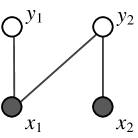
$$\mbox{\boldmath$G$}=\begin{bmatrix}1&1\\ 0&1\\ \end{bmatrix}$$

Figure 2: A simple mixture model. Hidden components are shown in white disks and observable components are shown in black disks.

Consider a simple mixture model with 2 hidden sources and 2 observables as depicted in Figure 2. The probability vector of the sources is $p=[\mbox{0.2 0.5}]$ with component $y_{1}$ having the lower probability being one. The marginal probabilities of $x_{1}=1$ and $x_{2}=1$ can be easily computed as 0.6 and 0.5, respectively. Let the realizations of $y_{1}$ and $y_{2}$ over ten trials be:

$$\mbox{\boldmath$Y$}=\begin{bmatrix}0&0&1&0&0&0&0&0&1&0\\ 0&1&1&0&0&1&1&1&0&0\end{bmatrix},$$

where $y_{it}=1$ indicates that source $y_{i}=1$ at the time slot $j$. $Y$ is hidden and unknown. Since $\mbox{\boldmath$G$}=\begin{bmatrix}1&1\\ 0&1\end{bmatrix}$, we have the observation matrix:

$$\mbox{\boldmath$X$}=\begin{bmatrix}0&1&1&0&0&1&1&1&1&0\\ 0&1&1&0&0&1&1&1&0&0\end{bmatrix}$$

The objective of bICA is to infer $G$ and $p$ from $X$. Since the number of observables $m=2$, we may identify at most $2^{m}-1=3$ unique sources, say, $\hat{y}_{1},\hat{y}_{2},\hat{y}_{3}$. Denote the inferred $G$ and $p$ as

$$\hat{\mbox{\boldmath$G$}}=\begin{bmatrix}1&0&1\\ 0&1&1\end{bmatrix},\hat{p}=\begin{bmatrix}\hat{p}_{1}&\hat{p}_{2}&\hat{p}_{3}\end{bmatrix},$$

In another word, component $\hat{y}_{1}$ only manifests through $x_{1}$, $\hat{y}_{2}$ through $x_{2}$, and $\hat{y}_{3}$ through both $x_{1}$ and $x_{2}$. Clearly, realizations in $X$ where $x_{2}=0$ correspond to time slots when sources $\hat{y}_{2}$ and $\hat{y}_{3}$ are both zero. In other words, we have

$$\mathcal{P}(x_{1}=1,x_{2}=0)=\hat{p}_{1}(1-\hat{p}_{2})(1-\hat{p}_{3}).$$

Note that $\mathcal{P}(x_{2}=0)=(1-\hat{p}_{2})(1-\hat{p}_{3})$. Therefore, we have $\hat{p}_{1}=\mathcal{P}(x_{1}=1|x_{2}=0)\approx 0.2$. The last term is estimated from the realization of $X$ where $x_{2}=0$. Since $x_{1}=1$ if $\hat{y}_{1}=1$ or $\hat{y}_{3}=1$, $\hat{p}_{3}$ can be calculated from

$$1-\mathcal{P}(x_{1}=1)=(1-\hat{p}_{1})(1-\hat{p}_{3})\Rightarrow\hat{p}_{3}=0.5.$$

Similarity, $\hat{p}_{2}$ can be calculated from

$$1-\mathcal{P}(x_{2}=1)=(1-\hat{p}_{2})(1-\hat{p}_{3})\Rightarrow\hat{p}_{2}=0.$$

$\hat{p}_{2}=0$ implies that $\hat{y}_{2}$ never activates, and thus its associated column can be removed from $\hat{\mbox{\boldmath$G$}}$.

The basic intuition of the above procedure is by limiting our considerations to realizations where some observables are zero, we “null” out the effects of components that contribute to these observations. This reduces the size of the inference problem to be considered.

The basic algorithm

Motivated by the above example, we will consider $G$ to be a $m\times 2^{m}$ adjacent matrix for the complete bipartite graph. Furthermore, the columns of $G$ are ordered such that $g_{kl}=1$ if $l\wedge 2^{k}=1$, for $k=1,\ldots,m$, where $\wedge$ is the bit-wise AND operator. As an example, when $m=3$ we have:

$$\mbox{\boldmath$G$}=\begin{bmatrix}0&1&0&1&0&1&0&1\\ 0&0&1&1&0&0&1&1\\ 0&0&0&0&1&1&1&1\end{bmatrix}$$

If the active probability of the $l$’th component $p_{l}=0$, this implies the corresponding column $\mbox{\boldmath$G$}_{:,l}$ can be removed from $G$. Before proceeding to the details of the algorithm, we first present a technical lemma.

Lemma 4

Consider a set $\mbox{$\mathbf{x}$}=[x_{1},x_{2},\ldots,x_{h-1},x_{h}]^{T}$ generated by the data model in (1), i.e., $\exists$ binary independent sources $\mathbf{y}$, s.t., $\mbox{$\mathbf{x}$}=\mbox{\boldmath$G$}\otimes\mbox{$\mathbf{y}$}$. The conditional random vector $\mbox{$\mathbf{x}$}_{x_{h}=0}=[x_{1},x_{2},\ldots,x_{h-1}|x_{h}=0]^{T}$ corresponds to the vector of the first $h-1$ elements of $\mathbf{x}$ when $x_{h}=0$. Then, $\mbox{$\mathbf{x}$}_{x_{h}=0}=\mbox{\boldmath$G$}^{\prime}\otimes\mbox{$\mathbf{y}$}^{\prime}$, where $\mbox{\boldmath$G$}^{\prime}=\mbox{\boldmath$G$}_{:,1\ldots 2^{h-1}}$ (i.e. the first $2^{h-1}$ columns of $G$) and $\mathcal{P}(y^{\prime}_{l}=1)=\mathcal{P}(y_{l}=1)$ for $l=1,\ldots,2^{h-1}$.

Proof:

We first derive the conditional probability distribution of the first $h-1$ observation variables given $x_{h}=0$,

$$\begin{array}[]{ll}&\mathcal{P}(x_{1},x_{2},\ldots,x_{h-1}\mid x_{h}=0)\\ =&\mathcal{P}(x_{1},x_{2},\ldots,x_{h-1}\mid x_{h}=0)\mathcal{P}(x_{h}=0)\\ \stackrel{{\scriptstyle(a)}}{{=}}&\displaystyle\sum_{\mbox{$\mathbf{y}$}\in Y(\mbox{$\mathbf{x}$})}{\prod_{l=1}^{2^{h}-1}{p_{l}^{y_{l}}(1-p_{l})^{1-y_{l}}}}\\ =&\displaystyle\sum_{\begin{array}[]{l}\mbox{$\mathbf{y}$}_{1..2^{h-1}}\in Y(\mbox{$\mathbf{x}$}_{1..h-1})\\ y_{l}=0,\forall g_{hl}=1\end{array}}{\prod_{g_{hl}=0}{p_{l}^{y_{l}}(1-p_{l})^{1-y_{l}}}\prod_{g_{hl}=1}{(1-p_{l})}}\end{array}$$ (7)

(a) is due to (4). Since $\mathcal{P}(x_{h}=0)=\displaystyle\prod_{g_{hl}=1}{(1-p_{l})}$, we have

$$\begin{array}[]{ll}&\mathcal{P}(x_{1},x_{2},\ldots,x_{h-1}\mid x_{h}=0)\\ =&\displaystyle\sum_{\mbox{$\mathbf{y}$}^{\prime}\in Y(\mbox{$\mathbf{x}$}_{1:h-1})}{\prod_{l=1}^{2^{h}-1}{(p^{\prime}_{l})^{y^{\prime}_{l}}(1-p^{\prime}_{l})^{1-y^{\prime}_{l}}}}\\ =&\displaystyle\sum_{\begin{array}[]{l}\mbox{$\mathbf{y}$}_{1,\ldots,2^{h-1}}\in Y(\mbox{$\mathbf{x}$}_{1,\ldots,h-1})\\ y_{l}=0,\forall g_{hl}=1\end{array}}{\prod_{g_{hl}=0}{p_{l}^{y_{l}}(1-p_{l})^{1-y_{l}}}.}\end{array}$$ (8)

Clearly, by setting $\mathcal{P}(y^{\prime}_{l}=1)=\mathcal{P}(y_{l}=1)$ for $l=1,\ldots,2^{h-1}$, the above equality holds. In the other word, the conditional random vector $\mbox{$\mathbf{x}$}_{x_{h}=0}=\mbox{\boldmath$G$}^{\prime}\otimes\mbox{$\mathbf{y}$}^{\prime}$ for $\mbox{\boldmath$G$}^{\prime}=\mbox{\boldmath$G$}_{:,1\ldots 2^{h-1}}$. ∎

The above lemma establishes that the conditional random vector $\mbox{$\mathbf{x}$}_{x_{h}=0}$ can be represented as an OR mixing of $2^{h-1}$ independent components. Furthermore, the set of the independent components is the same as the first $2^{h-1}$ independent components of $\mathbf{x}$ (under proper ordering).

Consider a sub-matrix of data matrix $X$, $\mbox{\boldmath$X$}_{(h-1)\times T}^{0}$, where the rows correspond to observations of $x_{1},x_{2},\ldots,x_{h-1}$ for $t=1,2,\ldots,T$ such that $x_{ht}=0$. Define $\mbox{\boldmath$X$}_{(h-1)\times T}$, which consists of the first $h-1$ rows of $X$. Suppose that we have computed the bICA for data matrices $\mbox{\boldmath$X$}_{(h-1)\times T}^{0}$ and $\mbox{\boldmath$X$}_{(h-1)\times T}$. From Lemma 4, we know that $\mbox{\boldmath$X$}_{(h-1)\times T}^{0}$ is realization of OR mixtures of independent components, denoted by $\mbox{$\mathbf{y}$}_{2^{h-1}}^{0}$. Furthermore, $\mathcal{P}[\mbox{$\mathbf{y}$}_{2^{h-1}}^{0}(l)=1]=\mathcal{P}(y_{l}=1)$ for $l=1,\ldots,2^{h-1}$. Clearly, $\mbox{\boldmath$X$}_{(h-1)\times T}$ is realization of OR mixtures of $2^{h-1}$ independent components, denoted by $\mbox{$\mathbf{y}$}_{2^{h-1}}$. Additionally, it is easy to see that the following holds:

$$\begin{array}[]{ll}&\mathcal{P}[\mbox{$\mathbf{y}$}_{2^{h-1}}(l)=1]\\ &=1-[1-\mathcal{P}(\mbox{$\mathbf{y}$}_{2^{h-1}}^{0}(l)=1)][1-\mathcal{P}(y_{l+2^{h-1}}=1)]\\ &=1-(1-p_{l})(1-p_{l+2^{h-1}}),\end{array}$$ (9)

where $l=1,\ldots,2^{h-1}$. Therefore,

$$\begin{array}[]{llll}p_{l}&=&\mathcal{P}(\mbox{$\mathbf{y}$}^{0}_{2^{h-1}}(l)=1),&l=1,\ldots,2^{h-1},\\ p_{l+2^{h-1}}&=&1-\frac{1-\mathcal{P}(\mbox{$\mathbf{y}$}_{2^{h-1}}(l)=1)}{1-\mathcal{P}(\mbox{$\mathbf{y}$}_{2^{h-1}}^{0}(l)=1)},&l=2,\ldots,2^{h-1},\\ p_{2^{h-1}+1}&=&\frac{\mathcal{F}{(x_{h}=1\wedge x_{i}=0,\forall i\in[1\ldots h-1])}}{\prod_{l=1\ldots 2^{h},l\neq 2^{h-1}-1}{(1-p_{l})}}.\end{array}$$ (10)

The last equation above holds because realizations of $\mathbf{x}$ where ($x_{k}=1$ while $x_{i}=0;\forall i\in\left\{0,\ldots,k-1\right\}$) are generated from OR mixtures of $\mbox{$\mathbf{y}$}_{2^{k-1}}$’s only.

Let $\mathcal{F}(A)$ be the frequency of event $A$, we have the iterative inference algorithm as illustrated in Algorithm 1.

FindBICA ($X$)

input : Data matrix $\mbox{\boldmath$X$}_{m\times T}$

init : $n=2^{m}-1$;

$p_{h}=0,h=1,\ldots,n$;

$G$ = $m\times(2^{m}-1)$ matrix with rows corresponding all possible binary vectors of length $m$;

$\varepsilon$ = the minimum threshold for $p_{h}$ to be considered a real component;

1if $m=1$ then

      2 $p_{1}=\mathcal{F}(x_{1}=0)$;

      3 $p_{2}=\mathcal{F}(x_{1}=1)$;

      

else

      4 if $\mbox{\boldmath$X$}^{0}_{(m-1)\times T}=\emptyset$ then

            5 $p_{1\ldots 2^{m-1}}$ = FindBICA ($\mbox{\boldmath$X$}_{(m-1)\times T}$);

            6 $p_{2^{m-1}+1}=1$;

            7 $p_{2^{m-1}+2\ldots 2^{m}}=0$;

            

      else

            8 $p_{1\ldots 2^{m-1}}$ = FindBICA ($\mbox{\boldmath$X$}^{0}_{(m-1)\times T}$);

            9 $p^{\prime}_{1\ldots 2^{m-1}}$ = FindBICA ($\mbox{\boldmath$X$}_{(m-1)\times T}$);

            10 for $l=2,\ldots,2^{m-1}$ do

                  11 $p_{l+2^{m-1}}=1-\frac{1-p^{\prime}_{l}}{1-p_{l}}$;

                  

            12 $p_{2^{m-1}+1}=\frac{\mathcal{F}{(x_{m}=1\wedge x_{i}=0,\forall i\in[1\ldots m-1])}}{\prod_{l=1\ldots 2^{m}-1,l\neq 2^{m-1}+1}{(1-p_{l})}}$;

            

      

13 for $h=1,\ldots,2^{m}$ do

      14 if $(p_{h}<\varepsilon)\vee(p_{h}=0)$ then

            15 prune $p_{h}$ and corresponding columns $g_{h}$;

            

      

16 output : $p$ and $G$

Algorithm 1 Incremental binary ICA inference algorithm

When the number of observation variables $m=1$, there are only two possible unique sources, one that can be detected by the monitor $x_{1}$, denoted by [1]; and one that cannot, denoted by [0]. Their active probabilities can easily be calculated by counting the frequency of $(x_{1}=1)$ and $(x_{1}=0)$ (lines 1 – 1). If $m\geq 2$, we apply Lemma 4 and (10) to estimate $p$ and $G$ through a recursive process. $\mbox{\boldmath$X$}^{0}_{(m-1)\times T}$ is sampled from columns of $X$ that have $x_{m}=0$. If $\mbox{\boldmath$X$}^{0}_{(m-1)\times T}$ is an empty set (which means $x_{mt}=1,\forall t$) then we can associate $x_{m}$ with a constantly active component and set the other components’ probability accordingly (lines 1 – 1). If $\mbox{\boldmath$X$}^{0}_{(m-1)\times T}$ is non-empty, we invoke FindBICA on two sub-matrices $\mbox{\boldmath$X$}^{0}_{(m-1)\times T}$ and $\mbox{\boldmath$X$}_{(m-1)\times T}$ to determine $p_{1\ldots 2^{m-1}}$ and $p^{\prime}_{1\ldots 2^{m-1}}$, then infer $p_{2^{m-1}+1\ldots 2^{m}}$ as in (10) (lines 1 – 1). Finally, $p_{h}$ and its corresponding column $g_{h}$ in $G$ are pruned in the final result if $p_{h}<\varepsilon$ (lines 1 – 1).

Reducing computation complexity

Let $S(m)$ be the computation time for finding bICA given $\mbox{\boldmath$X$}_{m\times T}$. From Algorithm 1, we have,

$$S(m)=2S(m-1)+c2^{m},$$

where $c$ is a constant. It is easy to verify that $S(m)=cm2^{m}$. Therefore, Algorithm 1 has an exponential computation complexity with respect to $m$. This is clearly undesirable for large $m$’s. However, we notice that in practice, correlations among $x_{i}$’s exhibit locality, and the $G$ matrix tends to be sparse. Instead of using a complete bipartite graph to represent $G$, the degree of vertices in $V$ (or the number of non-zero elements in $\mbox{\boldmath$G$}_{:,k}$) tend to be much less than $m$. In what follows, we discuss a few techniques to reduce the computation complexity by discovering and taking advantage of the sparsity of $G$. We first establish a few technical lemmas.

Lemma 5

If $x_{i}$ and $x_{k}$ are uncorrelated, then $\mathcal{P}(y_{l}=1)=0$, $\forall l$ s.t., $g_{il}=1$ and $g_{kl}=1$.

Proof:

We prove by contradiction. Suppose $\exists l$, s.t., $g_{il}=1$, $g_{kl}=1$, and $\mathcal{P}(y_{l}=1)=0$. Denote the $l$’s by a set $L$. Let $u=\wedge_{l\in L}y_{l}$. From the assumption, $u$ is non-degenerate. Without loss of generality, we can represent $x_{i}$ and $x_{k}$ as

$$x_{i}=u\vee v_{1}$$

$$x_{k}=u\vee v_{2}$$

where $v_{1}$ and $v_{2}$ are disjunctions of remaining non-overlapping components in $x_{i}$ and $x_{k}$, respectively From Lemma 3, we know that $x_{i}$ and $x_{k}$ are correlated. This contradicts the condition. ∎

Lemma 6

Consider the conditional random vector $\mbox{$\mathbf{x}$}_{x_{k}=0}=[x_{1},x_{2},\ldots,x_{k-1}|x_{k}=0]^{T}$ from a set $\mbox{$\mathbf{x}$}=[x_{1},x_{2},\ldots,x_{k-1},x_{k}]^{T}$ generated by the data model in (1). If $x_{i}$ and $x_{k}$ are uncorrelated, $\mbox{$\mathbf{x}$}_{x_{k}=0}(i)$ and $\mbox{$\mathbf{x}$}_{x_{k}=0}(k)$ are uncorrelated.

Proof:

This lemma is a direct consequence of Lemma 4 and Lemma 5. ∎

Lemma 5 implies that pair-wise independence can be used to eliminate edges/columns in $G$. Lemma 6 states that the pair-wise independence remains true for conditional vectors. Therefore, we can treat the conditional vectors similarly as the original ones.

We also observe that for $\mbox{$\mathbf{x}$}=[x_{1},x_{2},\ldots,x_{k-1},x_{k}]^{T}$ if (11) holds then there does not exist an independent component that generates $x_{k}$ and some of $x_{j}$, $j=1,2,\ldots k-1$. In other words, $x_{k}$ is generated by a “separate” independent component.

$$\mathcal{P}(x_{1},x_{2},\ldots,x_{k-1},x_{k})=\mathcal{P}(x_{1},x_{2},\ldots,x_{k-1})P(x_{k})$$ (11)

Finally from (9), we see that $\mathcal{P}(y_{k-1}(l)=1)\geq\max(p_{l},p_{l+2^{k-1}})$. Note that $\mathcal{P}(y_{k-1}(l)=1)$ is inferred from $\mbox{\boldmath$X$}_{(k-1)\times T}$, while the latter two are for $\mbox{\boldmath$X$}_{k\times T}$. This property allows us to prune the $G$ matrix along with the iterative procedure (as opposed to at the very end).

Now we are in the position to outline our complexity reduction techniques.

• For every pair $i$ and $k$, compute

  $$Cov(i,k)=\frac{\sum_{t}^{T}{\mbox{\boldmath$X$}_{it}\mbox{\boldmath$X$}_{kt}}}{T}-\frac{\sum_{t}^{T}{\mbox{\boldmath$X$}_{it}}}{T}\frac{\sum_{t}^{T}{\mbox{\boldmath$X$}_{kt}}}{T}.$$

  Let the associated $p$-value be $p(i,k)$. The basic idea of $p$-value is to use the original paired data $(\mbox{\boldmath$X$}_{i},\mbox{\boldmath$Y$}_{i})$, randomly redefining the pairs to create a new data set and compute the associated $r$-values. The p-value for the permutation is proportion of the $r$-values generated that are larger than that from the original data. If $p(i,k)>\epsilon$, where $\epsilon$ is a small value (e.g., 0.05), we can remove the corresponding columns in $G$ and elements in $\mathbf{y}$.

• We can determine the bICA for each sub-vector separately if the following holds,

  $$\mathcal{P}(x_{1},\ldots,x_{k})=\mathcal{P}(x_{1},\ldots,x_{l})\mathcal{P}(x_{1+1},\ldots,x_{k}).$$

• If the probability of the $i$’th component of $\mbox{\boldmath$X$}_{k\times T}$ $p_{i}<\epsilon$, then $\forall j$, s.t., $\mbox{\boldmath$G$}_{:,i}\prec\mbox{\boldmath$G$}_{:,j}$, the probability of the $j$’th component of $\mbox{\boldmath$X$}_{k^{\prime}\times T}$ $p_{j}<\epsilon$ for $k^{\prime}>k$. In another word, these columns and corresponding components can be eliminated.

From our evaluation study, we find the computation time is on the order of seconds for a problem size $m=20$ on a regular desktop PC.

V The Inverse Problem

Now we have the mixing matrix $\mbox{\boldmath$G$}_{m\times n}$ and the active probabilities $\mathcal{P}(\mbox{$\mathbf{y}$})$, given observation $\mbox{\boldmath$X$}_{m\times T}$, the inverse problem concerns inferring the realizations of the latent variables $\mbox{\boldmath$Y$}_{n\times T}$. Recall that $n$ is the number of latent variables. Denote $y_{i}$ to be the binary variable for the $i$’th latent variable. Let $\mbox{$\mathbf{x}$}=\mbox{\boldmath$G$}\otimes\mbox{$\mathbf{y}$}$. We assume that the probability of observing $X$ given $\mathbf{x}$ depends on their Hamming distance $d(\mbox{$\mathbf{x}$},\mbox{\boldmath$X$})=\sum_{i}{|\mbox{\boldmath$X$}_{i}-x_{i}|}$, and $\mathcal{P}(\mbox{$\mathbf{x}$}|\mbox{\boldmath$X$})=p_{e}^{d(\mbox{$\mathbf{x}$},\mbox{\boldmath$X$})}(1-p_{e})^{m-d(\mbox{$\mathbf{x}$},\mbox{\boldmath$X$})}$, where $p_{e}$ is the error probability of the binary symmetric channel. To determine $\mathbf{y}$, we can maximize the posterior probability of $\mathbf{y}$ given $X$ derived as follows,

$$\begin{array}[]{lll}\mathcal{P}\{\mbox{$\mathbf{y}$}|\mbox{\boldmath$X$}\}&=&\frac{\mathcal{P}\{\mbox{\boldmath$X$}|\mbox{$\mathbf{y}$}\}\mathcal{P}\{\mbox{$\mathbf{y}$}\}}{\mathcal{P}\{\mbox{\boldmath$X$}\}}\\ &=&\frac{\mathcal{P}\{\mbox{\boldmath$X$}|\mbox{$\mathbf{y}$}\}\mathcal{P}\{\mbox{$\mathbf{y}$}\}}{\mathcal{P}\{\mbox{\boldmath$X$}\}}\\ &\stackrel{{\scriptstyle(a)}}{{=}}&\frac{\mathcal{P}\{\mbox{\boldmath$X$},\mbox{$\mathbf{x}$}|\mbox{$\mathbf{y}$}\}\mathcal{P}\{\mbox{$\mathbf{y}$}\}}{\mathcal{P}\{\mbox{\boldmath$X$}\}}\\ &\stackrel{{\scriptstyle(b)}}{{=}}&\frac{\mathcal{P}\{\mbox{\boldmath$X$}|\mbox{$\mathbf{x}$}\}\mathcal{P}\{\mbox{$\mathbf{y}$}\}}{\mathcal{P}\{\mbox{\boldmath$X$}\}}\\ &=&\frac{\prod_{i=1}^{m}{\mathcal{P}\{\mbox{\boldmath$X$}_{i}|x_{i}\}}\prod_{j=1}^{n}{\mathcal{P}\{y_{i}\}}}{\mathcal{P}\{\mbox{\boldmath$X$}\}}\\ &=&\frac{\prod_{i=1}^{m}{p_{e}^{|x_{i}-\mbox{\boldmath$X$}|}(1-p_{e})^{1-|x_{i}-\mbox{\boldmath$X$}|}}\prod_{j=1}^{n}{p_{i}^{y_{i}}(1-p_{i})^{1-y_{i}}}}{\mathcal{P}\{\mbox{\boldmath$X$}\}}\end{array}$$

where $\mbox{$\mathbf{x}$}=\mbox{\boldmath$G$}\otimes\mbox{$\mathbf{y}$}$. $(a)$ and $(b)$ are due to the deterministic relationship between $\mathbf{x}$ and $\mathbf{y}$. Recall that $x_{i}=\bigvee_{j=1}^{n}{(g_{ij}\wedge y_{j})},i=1,\ldots,m$. With $M$ is a “large enough” constant, we can use big-$M$ formulation [14] to relax the disjunctive set and convert the above relationship between $\mathbf{x}$ and $\mathbf{y}$ into the following two sets of conditions:

$$\begin{array}[]{llll}\displaystyle x_{i}&\leq&\sum_{j=1}^{n}{g_{ij}y_{j}},\mbox{ }\forall i=1,\ldots,m.\\ \displaystyle M\cdot x_{i}&\geq&\sum_{j=1}^{n}{g_{ij}y_{j}},\mbox{ }\forall i=1,\ldots,m.\\ \end{array}$$ (12)

Here, since $\sum_{j=1}^{n}{g_{ij}y_{j}}\leq n$, we can set $M=n$. Finally, taking $\log$ on both sides and introducing additional auxiliary variable $\alpha_{i}=|\mbox{\boldmath$X$}_{i}-x_{i}|$, we have the the following integer programming problem:

$$\begin{array}[]{lll}\underset{\alpha,y}{\max.}&\displaystyle\sum_{i=1}^{m}{\left[\alpha_{i}\log{p_{e}}+(1-\alpha_{i})\log(1-p_{e})\right]}\\ &+\sum_{j=1}^{n}{\left[(1-y_{j})\log{(1-p_{j})}+y_{j}\log{p_{j}}\right]}\\ \mbox{s.t.}&\displaystyle x_{i}\leq\sum_{j=1}^{n}{g_{ij}y_{j}},\hskip 28.45274pt\forall i=1,\ldots,m,\\ &\displaystyle n\cdot x_{i}\geq\sum_{j=1}^{n}{g_{ij}y_{j}},\hskip 15.649pt\forall i=1,\ldots,m,\\ &\alpha_{i}\geq\mbox{\boldmath$X$}_{i}-x_{i},\hskip 31.29802pt\forall i=1,\ldots,m,\\ &\alpha_{i}\geq x_{i}-\mbox{\boldmath$X$}_{i},\hskip 31.29802pt\forall i=1,\ldots,m,\\ &\alpha_{i},x_{i},y_{j}=\left\{0,1\right\},\hskip 12.80373pt\forall i=1,\ldots,m,j=1,\ldots,n.\\ \end{array}$$ (13)

This optimization function can be solved using ILP solvers. Note that $p_{e}$ can be thought of the penalty for mismatches between $x_{i}$ and $\mbox{\boldmath$X$}_{i}$.

Zero Error Case

If $X$ is perfectly observed, containing no noise, we have $p_{e}=0$ and $\alpha_{i}=\mbox{$\mathbf{x}$}_{i}-\mbox{\boldmath$X$}_{i}=0$, or equivalently, $\mbox{$\mathbf{x}$}_{i}=\mbox{\boldmath$X$}_{i}$. The integer programming problem in (13) can now be simplified as:

$$\begin{array}[]{lll}\underset{y}{\max.}&\displaystyle\sum_{j=1}^{n}{\left[(1-y_{j})\log{(1-p_{j})}+y_{j}\log{p_{j}}\right]}\\ \mbox{s.t.}&\displaystyle\mbox{\boldmath$X$}_{i}\leq\sum_{j=1}^{n}{g_{ij}y_{j}},\hskip 28.45274pt\forall i=1,\ldots,m,\\ &\displaystyle n\cdot\mbox{\boldmath$X$}_{i}\geq\sum_{j=1}^{n}{g_{ij}y_{j}},\hskip 14.22636pt\forall i=1,\ldots,m,\\ &y_{j}=\left\{0,1\right\},\hskip 42.67912pt\forall j=1,\ldots,n.\\ \end{array}$$ (14)

Clearly, the computation complexity of the zero error case is lower compared to (13). It can also be used in the case where prior knowledge regarding the noise level is not available.

VI Evaluation

In this section, we first introduce performance metrics used for the evaluation of the proposed method, and then present its performance under different network topologies with different level of observation noises. In evaluating the structural errors of bICA, we also make an independent contribution by devising a matching algorithm for two bipartite graphs.

We compare the proposed algorithm with the Multi-Assignment Clustering (MAC) algorithm [7]. The source code of MAC was obtained from the authors’ web site. As shown in Table II, none of existing algorithms follows exactly the same model and/or constraints as bICA. For instance, MAC assumes the knowledge of the dimension of latent variables. Therefore, the comparisons bias against our proposed algorithm.

VI-A Evaluation metrics

We denote by $\hat{p}$ and $\hat{\mbox{\boldmath$G$}}$ the inferred active probability of latent variables and the inferred mixing matrix, respectively.

VI-A1 In Degree Error & Structure Error

Let $\|\cdot\|_{1}$ be the 1-norm defined by $\|x\|_{1}=\sum_{i=1}^{n}\sum_{j=1}^{m}{|x_{ij}|}$. $diag(\cdot)$ and $triu(\cdot)$ denote the main diagonal and the upper triangular portion of a matrix, respectively. Two metrics are introduced in [5] to evaluate the dissimilarity of $G$ and $\hat{\mbox{\boldmath$G$}}$. In degree error $E_{d}$ is the difference between the true in-degree of $G$ and the expected in-degree $\hat{\mbox{\boldmath$G$}}$. It is computed by taking the sum absolute difference between $diag(\mbox{\boldmath$G$}\mbox{\boldmath$G$}^{T})$ and $diag(\hat{\mbox{\boldmath$G$}}\hat{\mbox{\boldmath$G$}}^{T})$ as the following:

$$\begin{array}[]{lll}E_{d}&\stackrel{{\scriptstyle\Delta}}{{=}}&\|diag(\mbox{\boldmath$G$}\mbox{\boldmath$G$}^{T})-diag(\hat{\mbox{\boldmath$G$}}\hat{\mbox{\boldmath$G$}}^{T})\|_{1}\end{array}$$ (15)

The second metric, structure error $E_{s}$ is the sum of absolute difference between the upper triangular portion of $\mbox{\boldmath$G$}\mbox{\boldmath$G$}^{T}$ and $\hat{\mbox{\boldmath$G$}}\hat{\mbox{\boldmath$G$}}^{T}$, defined as:

$$\begin{array}[]{lll}E_{s}&\stackrel{{\scriptstyle\Delta}}{{=}}&\|triu(\mbox{\boldmath$G$}\mbox{\boldmath$G$}^{T})-triu(\hat{\mbox{\boldmath$G$}}\hat{\mbox{\boldmath$G$}}^{T})\|_{1}\end{array}$$ (16)

Since each element of the upper triangular portion of $\mbox{\boldmath$G$}\mbox{\boldmath$G$}^{T}$ is a count of the number of hidden causes shared by a pair of observable variables, the sum difference is a general measure of graph dissimilarity.

VI-A2 Normalized Hamming Distance

This metric indicates how accurate the mixing matrix is estimated. It is defined by the Hamming distance between $G$ and $\hat{\mbox{\boldmath$G$}}$ divided by its size.

$$\begin{array}[]{lll}\bar{H}_{g}&\stackrel{{\scriptstyle\Delta}}{{=}}&\frac{1}{mn}\sum_{i=1}^{n}d^{H}(\mbox{\boldmath$G$}_{:,i},\hat{\mbox{\boldmath$G$}}_{:,i}).\end{array}$$ (17)

To estimate $\bar{H}_{g}$ however, two challenges remain: First, the number of inferred independent components may not be identical as the ground truth. Second, the order of independent components in $G$ and $\hat{\mbox{\boldmath$G$}}$ may be different.

To solve the first problem, we can either prune $\hat{\mbox{\boldmath$G$}}$ or introduce columns into $G$ to equalize the number of components ($n=\hat{n}$, where $\hat{n}$ is the number of columns in $\hat{\mbox{\boldmath$G$}}$). For the second problem, we propose a matching algorithm that minimizes the Hamming distance between $G$ and $\hat{\mbox{\boldmath$G$}}$ by permuting the corresponding columns in $\hat{\mbox{\boldmath$G$}}$.

Structure Matching Problem

A naive matching algorithm needs to consider all $\hat{n}!$ column permutations of $\hat{\mbox{\boldmath$G$}}$, and chooses the one that has the minimal Hamming distance to $G$. This approach incurs an exponential computation complexity. Next, we first formulate the best match as an Integer Linear Programming problem. Denote the Hamming distance between column $\hat{\mbox{\boldmath$G$}}_{:,i}$ and $\mbox{\boldmath$G$}_{:,j}$ as $c_{ij}\geq 0$. Define a permutation matrix $\mbox{\boldmath$A$}_{n\times n}$ with $a_{ij}=1$ indicating that the $i$’th column in $\hat{\mbox{\boldmath$G$}}$ is matched with the $j$’th column in $G$. The problem now is to find a permutation matrix such that the total Hamming distance between $G$ and $\hat{\mbox{\boldmath$G$}}$ (denoted by $d^{H}(\mbox{\boldmath$G$},\hat{\mbox{\boldmath$G$}})$) is minimized. We can formulate this problem as an ILP as follows:

$$\begin{array}[]{ll}\underset{a}{\min.}&\displaystyle\sum_{i=1}^{n}{\sum_{j=1}^{n}{c_{ij}a_{ij}}}\\ \mbox{s.t.}&\displaystyle\sum_{i=1}^{n}{a_{ij}}=1,\\ &\displaystyle\sum_{j=1}^{n}{a_{ij}}=1,\\ &a_{ij}=\left\{0,1\right\},\hskip 14.22636pt\forall i,j=1,\ldots,n.\end{array}$$ (18)

MatchPG ($G$, $\hat{\mbox{\boldmath$G$}}$, $\hat{p}$)

input : $\mbox{\boldmath$G$}_{m\times n}$, $\hat{\mbox{\boldmath$G$}}_{m\times\hat{n}}$, $\hat{p}_{1\times\hat{n}}$; ($n\leq\hat{n}\leq 2^{m}$)

init : $\hat{\mbox{\boldmath$G$}}^{\prime}_{m\times\hat{n}}=0$; $\hat{p}^{\prime}_{1\times\hat{n}}=0$; $\mbox{\boldmath$C$}_{\hat{n}\times\hat{n}}=0$;

1 for $i=1,\ldots,\hat{n}$ do

      2 for $j=1,\ldots,\hat{n}$ do

            3 if $g_{i}=0$ then

                  4 $c_{ij}=d^{H}(\mbox{\boldmath$G$}_{:,i},\hat{\mbox{\boldmath$G$}}_{:,j})\times m$;

                  

            else

                  5 $c_{ij}=d^{H}(\mbox{\boldmath$G$}_{:,i},\hat{\mbox{\boldmath$G$}}_{:,j})$;

                  

            

      

6 $A$ = BipartiteMatching ($C$);

7 for $i=1,\ldots,\hat{n}$ do

      8 find $j$ such that $a_{ij}=1$;

      9 $\hat{\mbox{\boldmath$G$}}^{\prime}_{:,i}=\hat{\mbox{\boldmath$G$}}_{:,j}$;

      10 $\hat{p}^{\prime}_{i}=\hat{p}_{j}$;

11 Prune $\hat{\mbox{\boldmath$G$}}^{\prime}$: $\hat{\mbox{\boldmath$G$}}^{\prime}=\hat{\mbox{\boldmath$G$}}^{\prime}_{:,1\ldots n}$;

12 Prune $\hat{p}^{\prime}$: $\hat{p}^{\prime}=\hat{p}^{\prime}_{1\ldots n}$;

13 output : $\hat{\mbox{\boldmath$G$}}^{\prime}$ and $\hat{p}^{\prime}$

Algorithm 2 Bipartite graph matching algorithm

The constraints ensure the resulting $A$ is a permutation matrix. This problem can be solved using ILP solvers. However, we observe that the ILP is equivalent to a maximum-weight bipartite matching problem. In the bipartite graph, the vertices are positions of the columns, and the edge weights are the Hamming distance of the respective columns. If we consider $d^{H}(\mbox{\boldmath$G$}_{:,i},\hat{\mbox{\boldmath$G$}}_{:,i})$, the Hamming distance between column $\mbox{\boldmath$G$}_{:,i}$ and $\hat{\mbox{\boldmath$G$}}_{:,i}$, to be the “cost” of matching $\hat{\mbox{\boldmath$G$}}_{:,i}$ to $\mbox{\boldmath$G$}_{:,i}$, then the maximum-weight bipartite matching problem can be solved in $O(n^{3})$ running time [15], where $n$ is the number of vertices. The algorithm requires $G$ and $\hat{\mbox{\boldmath$G$}}$ to have the same number of columns.

One greedy solution is to prune $\hat{\mbox{\boldmath$G$}}$ by selecting the top $n$ components from $\hat{\mbox{\boldmath$G$}}$, which have the highest associated probabilities $\hat{p}_{i}$ since they are the most likely true components. However, when $T$ is small and/or under large noise, we may not have sufficient observations to correctly identify components in $G$ with high confidence. As a result, true components might have lower active probabilities comparing to the noise components. To address the problem, we instead keep a larger $\hat{n}$ and introduce $\hat{n}-n$ artificial components into $G$. These components will be represented by zero columns in $G$. While matching the inferred columns in $\hat{\mbox{\boldmath$G$}}$ to the columns in $G$, clearly an undesirable scenario occurs when we accidently match a column in $\hat{\mbox{\boldmath$G$}}$ to an additive zero column in $G$. This happens when an inferred column $\hat{\mbox{\boldmath$G$}}_{:,i}$ is sparse (i.e. having a very small Hamming distance to the zero column). To avoid the incident, we multiply the cost of matching any column in $\hat{\mbox{\boldmath$G$}}$ to a zero column in $G$ by $m$. This eliminates the case in which a column $\hat{\mbox{\boldmath$G$}}_{:,i}$ is matched with a zero column in $G$, since it is more expensive than matching with another non-zero column $\mbox{\boldmath$G$}_{:,i}$. We can now select the best $n$ candidates in $\hat{\mbox{\boldmath$G$}}$, which yields a reduced mixing matrix $\hat{\mbox{\boldmath$G$}}^{\prime}$ of size $m\times n$, and elements in active probability vector $\hat{p}^{\prime}$ will also be selected accordingly. The solution to the structure matching problem is detailed in Algorithm 2.

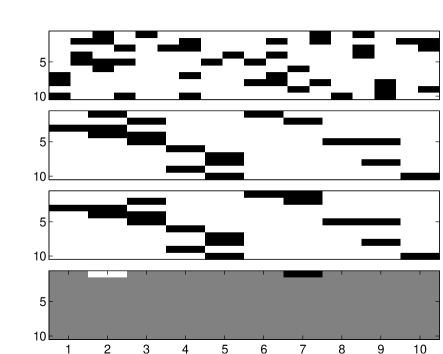
Figure 3: From top to bottom: inferred matrix $\hat{\mbox{\boldmath$G$}}$ with 18 inferred components, transformed matrix $\hat{\mbox{\boldmath$G$}}^{\prime}$ with only 10 components remaining (8 noisy ones were removed), original $G$ and difference matrix between $G$ and $\hat{\mbox{\boldmath$G$}}^{\prime}$. Black dot = 1 and white dot = 0.

In the algorithm, lines 2 – 2 build the input weight matrix $\mbox{\boldmath$C$}_{\hat{n}\times\hat{n}}$ for the bipartite matching algorithm. If $\mbox{\boldmath$G$}_{:,i}$ is a zero column, $c_{ij}$ will be scaled by $m$ to avoid the matching between column $\mbox{\boldmath$G$}_{:,i}$ and $\hat{\mbox{\boldmath$G$}}_{:,j}$ (line 2). The bipartite matching algorithm finds the optimal permutation matrix $A$ to transform $\hat{\mbox{\boldmath$G$}}$ into $\hat{\mbox{\boldmath$G$}}^{\prime}$ that is “closest” to $G$ (lines 2 – 2). We are only interested in the first $n$ columns of $\hat{\mbox{\boldmath$G$}}^{\prime}$ and $\hat{p}^{\prime}$ (as they most likely represent the true PUs). Therefore, $\hat{\mbox{\boldmath$G$}}^{\prime}$ and $\hat{p}^{\prime}$ are pruned in lines 2 – 2.

As an example, the inferred result of a random network with $n=m=10$ is given in Figure 3. Non-zero entries and zero entries of $G$, $\hat{\mbox{\boldmath$G$}}$, and $\hat{\mbox{\boldmath$G$}}^{\prime}$ are shown as black and white dots, respectively. The entry-wise difference matrix $|\mbox{\boldmath$G$}-\hat{\mbox{\boldmath$G$}}^{\prime}|$ is given in the bottom graph. Gray dots in the difference matrix indicate identical entries in the inferred $\hat{\mbox{\boldmath$G$}}$ and the original $G$; and black dots indicate different entries (and thus errors in the inferred matrix). In this case, only the first row (corresponding to the first monitor $x_{1}$) contains some errors.

VI-A3 Transmission Probability Error

The prediction error in the inferred transmission probability of independent users is measured by the Kullback-Leibler divergence between two probability distributions $p$ and $\hat{p}$. Let $p^{\prime}$ and $\hat{p}^{\prime}$ denotes the “normalized” $p$ and $\hat{p}$ ($p^{\prime}_{i}=p_{i}\sum_{i=1}^{n}p_{i}$), Transmission Probability Error is defined as below (the K-L distance):

$$\begin{array}[]{lll}\bar{P}(p^{\prime},\hat{p}^{\prime})&\stackrel{{\scriptstyle\Delta}}{{=}}&\sum_{i=1}^{n}p_{i}\log(\frac{p_{i}^{\prime}}{\hat{p_{i}}^{\prime}}).\end{array}$$ (19)

Intuitively, Transmission Probability Error gets larger as the predicted probability distribution $\hat{p}$ deviates more from the real distribution $p$.

VI-A4 Activity Error Ratio

After applying FindBICA in Algorithm 1 on the measurement data of length $T$ to obtain $\hat{\mbox{\boldmath$G$}}$ and $\hat{p}$, realizations of the hidden variables can be computed by solving the maximum likelihood estimation problem in (13). We define

$$\begin{array}[]{lll}\bar{H}_{y}&\stackrel{{\scriptstyle\Delta}}{{=}}&\frac{1}{nT}\sum_{i=1}^{T}d^{H}(\mbox{\boldmath$Y$}_{:,i},\hat{\mbox{\boldmath$Y$}}_{:,i}),\end{array}$$ (20)

where $\mbox{\boldmath$Y$}_{:,i}$ is the $i$’th column of $Y$. Similar to $\bar{H}_{g}$, this metric measures how accurately the activity matrix is inferred by calculating the ratio between the size of $\mathbf{y}$ and the absolute difference between $\mathbf{y}$ and $\hat{\mbox{$\mathbf{y}$}}$.

VI-B Experiment Results

(a)
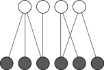
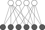
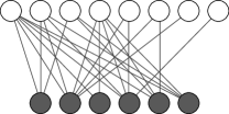
(b)
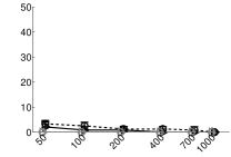
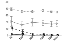
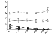
(c)
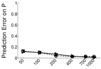
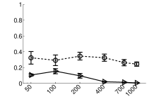
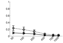
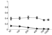
(d)
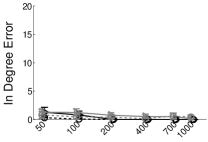
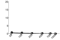
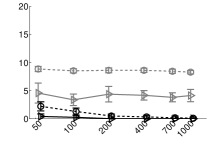
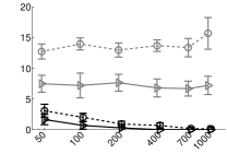
(e)
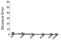
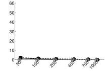
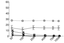
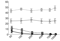
(f)
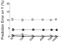
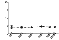
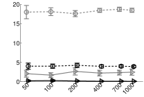
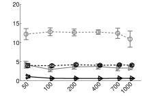
(g)

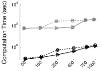
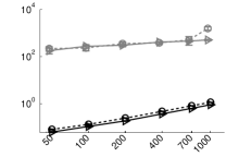
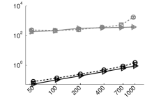
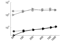
(i)

(ii)

(iii)

(iv)

Figure 4: Experiment result for bICA and MAC with fixed network topologies. Black lines are bICA performance while gray lines are MAC performance. The top row shows the four network topologies. The second to fifth rows show the mean Normalized Hamming Distance, Transmission Probability Error, In Degree Error, Structure Error and Activity Error Ratio of four topologies as $T$ increases from 50 to 1,000. On the last row is mean CPU runtime measured in seconds. Each graph shows experiment results at 2 different levels of noise: 0% and 10%. Error bars are symmetric, and indicate standard deviation over 50 runs with different initialized seeds.

We have implemented the proposed algorithm in Matlab. Four network topologies are manually created (Fig. 4(a)) representing different scenarios: connected vs. disconnected network, under-determined ($m>n$) vs. over-determined network ($m<n$). All experiments are conducted on a workstation with an Intel Core 2 Duo T5750@2.00GHz processor and 2GB RAM. For each scenario, 50 runs are executed; the results presented are the average value and 99% confidence interval. To evaluate the robustness of the interference algorithm, two different levels of noise are introduced, i.e. $p_{e}$ = 0% and 10%. In our experiment, noise is generated by randomly flipping an entry of the observation matrix $X$ with probability $p_{e}$.

Evaluation results for bICA and MAC at the two noise levels are presented in Fig. 4(b), (d), (e), and (f). We do not include the results of MAC in Fig. 4(c) since it does not infer the active probability for hidden components. From Fig. 4(b), we observe at zero noise, bICA converges quickly to the ground truth, and $G$ matrix has been accurately estimated with only 100 observations. bICA is comparable to or slightly outperforms MAC in the first two topologies, and significantly outperform MAC on the later two. It appears the MAC is quite sensitive to noise even in small structures. In contrast, the accuracy of bICA under 10% noise degrades when the number of the observations is small but improves significantly as more observations are available. Thus, bICA is more resilient to noise than MAC. As shown in Fig. 4(d) and (e), inference errors tend to increase with the same number of observations for both schemes as the structure become more complex for both schemes. However, bICA only degrades gracefully.

Fig. 4(f) shows the accuracy of the solution to the inverse problem. In this set of experiments, we first determine $\hat{\mbox{\boldmath$G$}}$ and $\hat{p}$ from the measurement data of length $T$. Then realizations of the hidden sources are estimated by solving the MLE problem in (13). The predication error is measured by the Activity Error Ratio. We see that at the 0% noise level, both methods perform quite well. Since the inference of each realization of $\mathbf{y}$ is independent from the others, increasing $T$ does not help improving the accuracy of the inverse problem (though higher T gives a better estimation of $G$ and $p$. Performance of both methods degrades as the noise level increases. Noise has two effects on the solution to inverse problem. First, the inferred mixing matrix and the active probability can be erroneous. Second, no maximum likelihood estimator guarantees to give the exact result when the problem is under or close to under-determined with noisy measurements. To verify the second argument, we provide the exact $G$ and $p$ to the MLE formulation, and observe comparable errors in the inferred $\mathbf{y}$ as the case where $G$ and $p$ are both inferred by bICA. This implies that the main source of errors in the inverse problem comes from the under-determined or close to under-determined name of the problem.

TABLE III: Average computation time (in seconds) of bICA and MAC over the 4 network topologies, 2 noise levels, and all sample sizes.

	Topology 1	Topology 2	Topology 3	Topology 4
bICA	0.49	0.38	0.38	0.64
MAC	166.5	289.21	302.35	538.47

Finally, from Fig. 4(g), the computation time of bICA is negligible (under 0.5 second in most cases and under 1.5 seconds in the worst case). For the ease of comparison, we list the numerical values in Table III. MAC uses a gradient descent optimization scheme, it is much more time-consuming. As mentioned earlier, the complexity of bICA is a function of $m$ and the sparsity of $G$. In practice, computation time of bICA is also a monotonic function of the number of observations $T$ and noise levels. As $T$ is getting larger, the storage and computation complexity tends to grow. When $T$ is small or the noise level is high, the structure inferred may error on the higher complexity side, resulting longer computation time.

VII Applications

In this section, we present some case studies on real-world application of bICA. In general, bICA can be applied to any problem that need identifying hidden source signals from binary observations. The proposed method therefore can find applications in many domains. In multi-assignment clustering [7], where boolean vectorial data can simultaneously belong to multiple clusters, the binary data can be modeled as the disjunction of the prototypes of all clusters the data item belongs to. In medical diagnosis, the symptoms of patients are explained as the result of diseases that are not themselves directly observable [5]. Multiple diseases can exhibit similar symptoms. In the Internet tomography [16], losses on end-to-end paths can be attributed to losses on different segments (e.g., edges) of the paths. In all above generic applications, the underlying data models can be viewed as disjunctions of binary independent components (e.g., membership of a cluster, presence of a disease, packet losses on a network edge, etc). Now we will introduce in detail two specific network applications in which bICA has been effectively applied.

VII-A Optimal monitoring for multi-channel wireless networks

Passive monitoring is a technique where a dedicated set of hardware devices called sniffers, or monitors, are used to monitor activities in wireless networks. These devices capture transmissions of wireless devices or activities of interference sources in their vicinity, and store the information in trace files, which can be analyzed distributively or at a central location. Most operational networks operate over multiple channels, while a single radio interface of a sniffer can only monitor one channel at a time. Thus, the important question is to decide the sniffer-channel assignment to maximize the total information (user transmitted packets) collected.

Network model and optimal monitoring

Consider a system of $m$ sniffers, and $n$ users, where each user $u$ operates on one of $K$ channels, $c(u)\in\mathcal{K}=\left\{1,\ldots,K\right\}$. The users can be wireless (mesh) routers, access points or mobile users. At any point in time, a sniffer can only monitor packet transmissions over a single channel. We represent the relationship between users and sniffers using an undirected bi-partite graph $G=(S,U,E)$, where $S$ is the set of sniffer nodes and $U$ is the set of users. An edge $e=(s,u)$ exists between sniffer $s\in S$ and user $u\in U$ if $s$ can capture the transmission from $u$. If transmissions from a user cannot be captured by any sniffer, the user is excluded from $G$. For every vertex $v\in U\cup S$, we let $N(v)$ denote vertex $v$’s neighbors in $G$. For users, their neighbors are sniffers, and vice versa. We will also refer to $G$ as the binary $m\times n$ adjacency matrix of graph $G$. An example network with sniffers and users, the corresponding bipartite graph $G$, and its matrix representation $G$ are given in Figure 5.

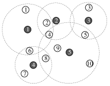
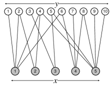
$$\mbox{\boldmath$G$}=\begin{bmatrix}1&\hskip 4.2679pt1&\hskip 4.2679pt0&\hskip 4.2679pt1&\hskip 4.2679pt0&\hskip 4.2679pt1&\hskip 4.2679pt0&\hskip 4.2679pt0&\hskip 4.2679pt0&\hskip 4.2679pt0\\ 0&\hskip 4.2679pt1&\hskip 4.2679pt0&\hskip 4.2679pt1&\hskip 4.2679pt0&\hskip 4.2679pt0&\hskip 4.2679pt0&\hskip 4.2679pt0&\hskip 4.2679pt0&\hskip 4.2679pt0\\ 0&\hskip 4.2679pt0&\hskip 4.2679pt1&\hskip 4.2679pt0&\hskip 4.2679pt1&\hskip 4.2679pt0&\hskip 4.2679pt0&\hskip 4.2679pt0&\hskip 4.2679pt0&\hskip 4.2679pt0\\ 0&\hskip 4.2679pt0&\hskip 4.2679pt0&\hskip 4.2679pt0&\hskip 4.2679pt0&\hskip 4.2679pt1&\hskip 4.2679pt1&\hskip 4.2679pt1&\hskip 4.2679pt0&\hskip 4.2679pt0\\ 0&\hskip 4.2679pt0&\hskip 4.2679pt0&\hskip 4.2679pt1&\hskip 4.2679pt1&\hskip 4.2679pt0&\hskip 4.2679pt0&\hskip 4.2679pt1&\hskip 4.2679pt1&\hskip 4.2679pt1\end{bmatrix}\begin{matrix}x_{1}\\ x_{2}\\ x_{3}\\ x_{4}\\ x_{5}\end{matrix}\vspace{-2mm}$$

$$\hskip 14.22636pt\begin{matrix}y_{1}&y_{2}&y_{3}&y_{4}&y_{5}&y_{6}&y_{7}&y_{8}&y_{9}&y_{10}\end{matrix}$$

Figure 5: A sample network scenario with number of sniffers $m=5$, number of users $n=10$, its bipartite graph transformation and its matrix representation. White circles represent independent users, black circles represent sniffers and dashed lines illustrate sniffers’ coverage range.

If we assume that $G$ is known by inspecting packet headers information from each sniffers’ captured traces, then the transmission probability of the users $p=(p_{u})_{u\in U}$ are available and are assumed to be independent. As mentioned earlier, the more complete information can be collected, the easier it is for a network administrator to make decisions regarding network troubleshooting. We can therefore measure the quality of monitoring by the total expected number of active users monitored by the sniffers. Our problem now is to find a sniffer assignment of sniffers to channels so that the expected number of active users monitored is maximized. It can be casted as the following integer program:

$$\begin{array}[]{rll}\underset{y,z}{\max.}&\sum_{u\in U}p_{u}y_{u}\\[5.69046pt] \mbox{s.t.}&\sum_{k=1}^{K}z_{s,k}\leq 1,&\quad\forall s\in S,\\ &y_{u}\leq\sum_{s\in N(u)}z_{s,c(u)},&\quad\forall u\in U,\\ &y_{u}\leq 1,&\quad\forall u\in U,\\ &y_{u},z_{s,k}\in\left\{0,1\right\},&\quad\forall u,s,k,\end{array}$$ (21)

where the binary decision variable $z_{s,k}=1$ if the sniffer is assigned to channel $k$; 0 otherwise. $y_{u}$ is a binary variable indicating whether or not user $u$ is monitored, and $p_{u}$ is the active probability of user $u$.

Network topology inference with binary observations

From (21), it is clear that we need the network and user-level information in order to maximize the quality of monitoring. However, this information is not always available. We consider binary sniffers, or sniffers that can only capture binary information (on or off) regarding the channel activity. Examples of such kind of sniffers are energy detection sensors using for spectrum sensing. The problem now is to infer the user-sniffer relationship (i.e. $G$) and the active probability of users from the observation data (i.e. $X$). Let $\mbox{$\mathbf{x}$}=[x_{1},x_{2},\ldots,x_{m}]^{T}$ be a vector of $m$ binary random variables and $X$ be the collection of $T$ realizations of $\mathbf{x}$, where $x_{it}$ denotes whether or not sniffer $s_{i}$ captures communication activities in its associated channel at time slot $t$. Let $\mbox{$\mathbf{y}$}=[y1,y2,\ldots,y_{n}]^{T}$ be a vector of $n$ binary random variables, where $y_{j}=1$ if user $u_{j}$ transmits in its associated channel, and $y_{j}=0$ otherwise. Sniffer observations are thus disjunctive mixtures of user activities. In other words, relationship between $\mathbf{x}$ and $\mathbf{y}$ is $\mbox{$\mathbf{x}$}=\mbox{\boldmath$G$}\otimes\mbox{$\mathbf{y}$}$ and thus we can use bICA to infer $G$ and $p$.

WiFi trace collection and evaluation result

We evaluate our proposed scheme by data traces collected from the University of Houston campus wireless network using 21 WiFi sniffers deployed in the Philip G. Hall. Over a period of 6 hours, between 12 p.m. and 6 p.m., each sniffer captured approximately 300,000 MAC frames. Altogether, 655 unique users are observed operating over three channels. The number of users observed on channels 1, 6, 11 are 382, 118, and 155, respectively. Most users are active less than 1% of the time except for a few heavy hitters. User-level information is removed leaving only binary channel observation from each sniffer. $G$ and $p$ are then inferred using bICA and input to the integer program (21) to find the best sniffer channel assignment that maximize the expected number of active users monitored. Obviously, the more accurate the network model is inferred, the better the assignment is and the more users are monitored. We also vary the result by randomly select a subset of sniffers and observe the number of monitored users from this set of sniffers. Result is presented in Fig. 6

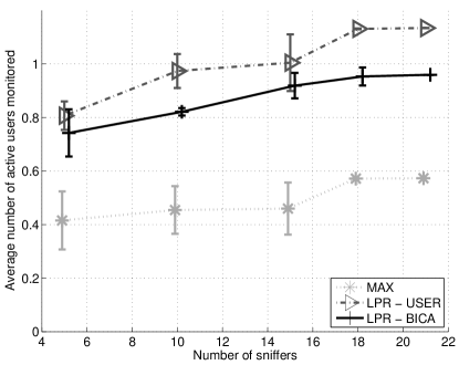
Figure 6: Expected number of active users monitored with the number of sniffers vary from 5 to 21.

In Fig. 6, we compare the average of number of active users monitored using the inferred $\hat{\mbox{\boldmath$G$}}$ and $\hat{p}$, and the ground truth. The integer programming problem (21) is solved using a random rounding procedure on its LP relaxation, which is shown to perform very close to the LP upper bound in our earlier work [17].

Note that most users are active less than 1% and the average active probability of users is 0.0014. The system consists of 655 unique users, therefore the average number of active users monitored is around 1. For comparison, we also include a naive scheme (Max) that puts each sniffer to its busiest channel. Therefore, Max does not infer or utilize any structure information. From Fig. 6, we observe that the sniffer-channel assignment scheme with bICA (LPR – BICA) performs close to the case when full information is available (LPR – USER), and much better than an agnostic scheme such as Max (MAX). This demonstrates that bICA can indeed recover useful structure information from the observations.

VII-B PU separation in cognitive radio networks

With tremendous growth in wireless services, the demand for radio spectrum has significantly increased. However, spectrum resources are scarce and most of them have been already licensed to existing operators. Recent studies have shown that despite claims of spectral scarcity, the actual licensed spectrum remains unoccupied for long periods of time [18]. Thus, cognitive radio (CR) systems have been proposed [19, 20, 21] in order to efficiently exploit these spectral holes, in which licensed primary users (PUs) are not present. CRs or secondary users (SUs) are wireless devices that can intelligently monitor and adapt to their environment, hence, they are able to share the spectrum with the licensed PUs, operating when the PUs are idle.

One key challenge in CR systems is spectrum sensing, i.e., SUs attempt to learn the environment and determine the presence and characteristics of PUs. Energy detection is one of the most commonly used method for spectrum sensing, where the detector computes the energy of the received signals and compares it to a certain threshold value to decide whether the PU signal is present or not. It has the advantage of short detection time but suffers from low accuracy compared to feature-based approaches such as cyclostationary detection [20, 21]. From the prospective of a CR system, it is often insufficient to detect PU activities in a single SU’s vicinity (“is there any PU near me?”). Rather, it is important to determine the identity of PUs (“who is there?”) as well as the distribution of PUs in the field (“where are they?”). We call these issues the PU separation problem. Clearly, PU separation is a more challenging problem compared to node-level PU detection.

Solving PU separation problem with bICA

Consider a slotted system in which the transmission activities of $n$ PUs are modeled as a set of independent binary variables $\mathbf{y}$ with active probabilities $\mathcal{P}(\mbox{$\mathbf{y}$})$. The binary observations due to energy detection at the $m$ monitor nodes are modeled as an $m$-dimension binary vector $\mbox{$\mathbf{x}$}=[x_{1},x_{2},\ldots,x_{m}]^{T}$ with joint distribution $\mathcal{P}(\mbox{$\mathbf{x}$})$. It is assumed that presence of any active PU surrounding of a monitor leads to positive detection. If we let a (unknown) binary mixing matrix $G$ represents the relationship between the observable variables in $\mathbf{x}$ and the latent binary variables in $\mbox{$\mathbf{y}$}=[y_{1},y_{2},\ldots,y_{n}]^{T}$, then we can write $\mbox{$\mathbf{x}$}=\mbox{\boldmath$G$}\otimes\mbox{$\mathbf{y}$}$. The PU separation is therefore amenable to bICA.

Inferring PU activities with the inverse problem

Extracting multiple PUs activities from the OR mixture observations is a challenging but important problem in cognitive radio networks. Interesting information, such as the PU channel usage pattern can be inferred once $Y$ is available. The SUs will then be able to adopt better spectrum sensing and access strategies to exploit the spectrum holes more effectively. Now suppose that we are given the observation matrix $X$ and already estimated the mixing matrix $G$ and the active probabilities $\mathcal{P}(\mbox{$\mathbf{y}$})$. Solving the inverse problem gives the PU activity matrix $Y$.

Simulation setup and result

In the simulation, 10 monitors and $n$ PUs are deployed in a 500x500 square meter area. We fix the sample size $T=10,000$ and vary the number of PUs from 5 to 20 to study its impact on the accuracy of our method. Locations of PUs are chosen arbitrarily on the field. The PUs transmit power levels are fixed at 20mW, the noise floor is -95dbm, and the propagation loss factor is 3. The SNR detection threshold for the monitors is set to be 5dB. PUs activities are modeled as a two-stage Markov chain with transition probabilities uniformly distributed over [0; 1]. A monitor reports the channel occupancy if any detectable PU is active. Noise is introduced by randomly flip a bit in the observation matrix $X$ from 1 to 0 (and vice versa) at probability $e$. $e$ is set at 0%, 2%, and 5%. Prediction error on $G$ and $Y$ over 50 runs for each PU setting are shown in Fig. 7.

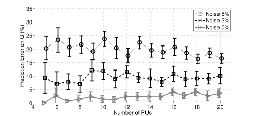
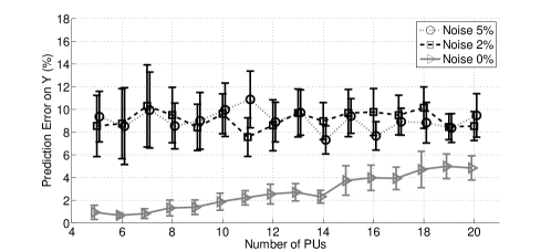
Figure 7: Inference error on $G$ and $Y$ at three noise levels.

As we can see, at noise level 0%, bICA can accurately estimate the underlying PU-SU relationship and the hidden PU activities for small number of PUs. However, introducing noise or having more PUs tend to degrade the performance of the inference scheme. The errors in the noisy cases can be attributed to the fact that the average PU active probability is around 2%, which is comparable to the noise level. More information on this application can be found in [22].

VIII Conclusion

In this paper, we provided a comprehensive study of the binary independent component analysis with OR mixtures. Key properties of bICA were established. A computational efficient inference algorithm have been devised along with the solution to the inverse problem. Compared to MAC, bICA is not only faster, but also more accurate and robust against noise. We have also demonstrated the use of bICA in two network applications, namely, optimal monitoring in multi-channel wireless networks and PU separation in cognitive radio networks. We believe the methodology devised can be useful in many other application domains.

As future work, we are interested in devising inference schemes that can easily incorporate priori knowledge of the structure or active probability of latent variables. Also on the agenda is to apply bICA to problems in application domains beyond wireless networks.

References

- [1] A. Hyvärinen and E. Oja, “Independent component analysis: algorithms and applications,” Neural Netw., vol. 13, no. 4-5, pp. 411–430, 2000.
- [2] A. Yeredor, “Ica in boolean xor mixtures,” in ICA, 2007, pp. 827–835.
- [3] A. Kabán and E. Bingham, “Factorisation and denoising of 0-1 data: a variational approach,” Neurocomputing, special, vol. 71, no. 10-12, 2009.
- [4] T. Šingliar and M. Hauskrecht, “Noisy-or component analysis and its application to link analysis,” J. Mach. Learn. Res., vol. 7, pp. 2189–2213, December 2006. [Online]. Available: http://portal.acm.org/citation.cfm?id=1248547.1248625
- [5] F. W. Computer and F. Wood, “A non-parametric bayesian method for inferring hidden causes,” in Proceedings of the Twenty-Second Conference on Uncertainty in Artificial Intelligence (UAI. AUAI Press, 2006, pp. 536–543.
- [6] T. L. Griffiths, T. L. Griffiths, Z. Ghahramani, and Z. Ghahramani, “Infinite latent feature models and the indian buffet process,” 2005.
- [7] A. P. Streich, M. Frank, D. Basin, and J. M. Buhmann, “Multi-assignment clustering for boolean data,” in ICML ’09: Proceedings of the 26th Annual International Conference on Machine Learning. New York, NY, USA: ACM, 2009, pp. 969–976.
- [8] K. Diamantaras and T. Papadimitriou, “Blind deconvolution of multi-input single-output systems with binary sources,” Signal Processing, IEEE Transactions on, vol. 54, no. 10, pp. 3720 –3731, October 2006.
- [9] Y. Li, A. Cichocki, and L. Zhang, “Blind separation and extraction of binary sources,” IEICE Trans. Fund. Electron. Commun. Comput. Sci., vol. E86-A, no. 3, p. 580–589, 2003.
- [10] A. A. Frolov, D. Húsek, I. P. Muraviev, and P. Y. Polyakov, “Boolean factor analysis by attractor neural network,” IEEE Transactions on Neural Networks, vol. 18, no. 3, pp. 698–707, 2007.
- [11] R. Belohlavek and V. Vychodil, “Discovery of optimal factors in binary data via a novel method of matrix decomposition,” J. Comput. Syst. Sci., vol. 76, pp. 3–20, February 2010. [Online]. Available: http://portal.acm.org/citation.cfm?id=1655426.1655707
- [12] D. Húsek, H. Rezanková, V. Snásel, A. A. Frolov, and P. Polyakov, “Neural network nonlinear factor analysis of high dimensional binary signals,” in SITIS, 2005, pp. 86–89.
- [13] D. Húsek, P. Moravec, V. Snásel, A. A. Frolov, H. Rezanková, and P. Polyakov, “Comparison of neural network boolean factor analysis method with some other dimension reduction methods on bars problem,” in PReMI, 2007, pp. 235–243.
- [14] I. Griva, S. G. Nash, and A. Sofer, Linear and Nonlinear Optimization, Second Edition, 2nd ed. Society for Industrial Mathematics, December 2008.
- [15] H. W. Kuhn, “The Hungarian method for the assignment problem,” Naval Research Logistic Quarterly, vol. 2, pp. 83–97, 1955.
- [16] R. Castro, M. Coates, G. Liang, R. Nowak, and B. Yu, “Network tomography: recent developments,” Statistical Science, vol. 19, pp. 499–517, 2004.
- [17] A. Chhetri, H. Nguyen, G. Scalosub, and R. Zheng, “On quality of monitoring for multi-channel wireless infrastructure networks,” in Proceedings of the eleventh ACM international symposium on Mobile ad hoc networking and computing, ser. MobiHoc ’10. New York, NY, USA: ACM, 2010, pp. 111–120.
- [18] Federal Communications Commission, “Spectrum policy task force report,” Report ET Docket no. 02-135, Nov. 2002.
- [19] J. Mitola and G. Q. Maguire, “Cognitive radio: Making software radios more personal,” IEEE Pers. Commun., vol. 6, pp. 13–18, Aug. 1999.
- [20] S. Haykin, “Cognitive radio: brain-empowered wireless communications,” IEEE JSAC, vol. 23, pp. 201–220, Feb. 2005.
- [21] D. Niyato, E. Hossein, and Z. Han, Dynamic spectrum access in cognitive radio networks. Cambridge, UK: Cambridge University Press, To appear 2009.
- [22] H. Nguyen, G. Zheng, Z. Han, and R. Zheng, “Binary inference for primary user separation in cognitive radio networks,” preprint (2010), available at http://arxiv.org/abs/1012.1095.