Interaction of a Nanomagnet with a Weak Superconducting Link

Abstract

We study electromagnetic interaction of a nanomagnet with a weak superconducting link. Equations that govern coupled dynamics of the two systems are derived and investigated numerically. We show that the presence of a small magnet in the proximity of a weak link may be detected through Shapiro-like steps caused by the precession of the magnetic moment. Despite very weak magnetic field generated by the weak link, a time-dependent bias voltage applied to the link can initiate a non-linear dynamics of the nanomagnet that leads to the reversal of its magnetic moment. We also consider quantum problem in which a nanomagnet interacting with a weak link is treated as a two-state spin system due to quantum tunneling between spin-up and spin-down states.

I Introduction

Josephson junctions and magnets in a close proximity of each other can be coupled through various mechanisms. Static properties of superconductor/ferromagnet/superconductor (S/F/S) Josephson junctions have been intensively studied in the past but not as much attention has been paid to the coupled dynamics of the magnetic moment and the tunneling current. The effect of superconductivity on ferromagnetic resonance in such junctions has been recently observed by Bell et al Bell-2008 who attributed their observation to the proximity effect Buzdin-review . Theory that may be relevant to this experiment has been worked out by Buzdin who computed the phase shift in the Josephson junction arising from the Rashba-type spin-orbit coupling Buzdin-2008 and studied the coupled dynamics of the magnetization and the Josephson current due to this mechanism Buzdin-2009 . Dynamical proximity effect generated by the precession of the magnetization in an S/F/S junction has been also investigated by Houzet Houzet-2008 Shapiro steps in the I-V curve of the S/F/S junction, related to the ferromagnetic resonance, have been reported by Petković et al Petkovic-2009 who also provided theoretical arguments favoring a purely electrodynamic nature of the effect in their experiment.

Coupling of Josephson junctions to individual spins inside the junction have been also intensively studied in the past. The theory traces back to the works of Kulik Kulik-1966 and Bulaevskii et al Bulaevskii-1977 who elucidated the effect of spin flips on the tunneling current. More recently, Nussinov et al Zhu-2004 ; Nussinov-2005 , using Keldysh formalism, demonstrated that superconducting correlations drastically change dynamics of a spin inside a Josephson junction. Josephson current through a multilevel quantum dot with spin-orbit coupling has been studied by Dell’Anna et al Anna-2007 . Deposition of a single magnetic molecule in a SQUID loop has been attempted Lam-2008 and theoretical treatments of the Josephson current through such a molecule have been proposed Benjamin-2007 ; Teber-2010 . Samokhvalov Samokhvalov-2009 considered formation of vortices in a Josephson junction by a magnetic dot. Spin-orbit coupling of a single spin to the Josephson junction has been studied by Padurariu and Nazarov Nazarov-2010 in the context of superconducting spin qubits. Somewhat related to single spins are also studies of two-level systems inside Josephson junctions two-level .

Early experimental research on coupling of magnetic nanoparticles to microSQUIDs has been reviewed by Wernsdorfer Wernsdorfer-2001 who also reviewed recent progress made due to the development of nanoSQUIDs Wernsdorfer-2009 . Thirion et al Thirion-2003 demonstrated the possibility of switching of the magnetization of 20nm Co nanoparticles in a dc magnetic field by the radio-frequency pulse generated by a microSQUID. They measured the angular dependence of the switching field and reproduced the Stoner-Wohlfarth astroid Lectures for a single nanoparticle. Further miniaturization of such systems has been achieved using carbon nanotubes Wern-CNT and nanolithography assisted by the atomic force microscope Faucher-2009 . Such systems utilizing single magnetic molecules have been proposed as possible ultimate memory units and as elements of quantum computers Wern-08 .

In this paper we consider a nanomagnet located close to a weak link between two superconductors, see Fig. 1.

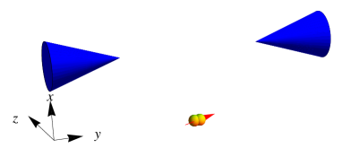
Figure 1: Color online: Nanomagnet near a weak superconducting link.

The position of the nanomagnet is away from the path of the tunneling current, so that the interaction between the two systems is considered to be of purely electromagnetic origin. The mechanism of the interaction is conceptually similar to that argued in the experiment of Ref. Petkovic-2009, . The magnetic field of the nanomagnet alters the Josephson current flowing through the link, while the magnetic flux generated by the Josephson junction acts on the magnetic moment of the nanomagnet. From mathematical point of view the dynamics of this problem resembles the dynamics studied in Ref. Buzdin-2009, . The differences stem from different geometry, different interaction, and finite normal resistance of the weak link that we allow within the RSJ model. The attractiveness of the problem that deals with purely electromagnetic interactions is in the absence of the unknown parameters. We hope that this will assist experimentalists in designing Josephson junction - nanomagnet systems with desired properties.

Dynamical equations describing the system depicted in Fig. 1 are derived in the next Section. Small oscillations of the magnetic moment of the nanomagnet caused by a constant voltage applied to the weak link are studied in Section III. We show that such oscillations can produce Shapiro-like steps in the I-V curve without any external ac voltage applied to the link. Non-linear dynamics of the nanomagnet due to a voltage pulse applied to the link is studied in Section IV. We show that using a specific slow time dependence of the voltage pulse one can reverse the magnetic moment of the nanomagnet. The remarkable feature of this process is that the reversal can be achieved despite the fact that the magnetic field generated by the link is small compared to the switching field determined by the magnetic anisotropy. This is similar to the effect of the RF field demonstrated experimentally in Ref. Thirion-2003, . The reversal occurs due to the pumping of spin excitations into the nanomagnet by the ac-field of the oscillating tunneling current. The final part of the paper studies electromagnetic interaction of the weak link with a quantum two-state system formed by tunneling of the nanomagnet’s spin between up and down orientations. Quantum dynamics of this system is derived in Section V. We show that it provides the simplest realization of a Josephson junction - spin qubit suggested in Ref. Nazarov-2010, (see also Ref. Wern-08, and Ref. qubit, ). Our conclusions and suggestions for experiment are summarized in Section VI.

II The Model

We consider a system depicted in Fig. 1. Nanomagnet of a fixed-length magnetic moment ${\bf M}$ is located at a distance $a$ from the center of the weak superconducting link of length $L$. The nanomagnet is assumed to be rigidly embedded in the solid matrix of the link. In the presence of the external magnetic field ${\bf B}_{0}$, the energy of the nanomagnet is then given by

$${\cal{E}}_{M}=K({\bf M})-{\bf M}\cdot{\bf B}_{0}\,,$$ (1)

where $K({\bf M})$ is the energy of the magnetic anisotropy that depends on the orientation of ${\bf M}$ with respect to the body of the magnet.

Neglecting the capacitance of the weak link, the energy of the link can be written as

$${\cal{E}}_{J}=-E_{J}\cos\gamma\,,$$ (2)

where $\gamma$ is the gauge invariant phase, $E_{J}=\hbar I_{c}/(2e)$ is the Josephson energy, and $I_{c}$ is the critical current of the link. Note that $E_{J}$ depends on the external field ${\bf B}_{0}$. Time derivative of $\gamma$,

$$\frac{d\gamma}{dt}=\frac{2eV(t)}{\hbar}\,,$$ (3)

is proportional to the total voltage,

$$V(t)=\int_{1}^{2}d{\bf r}\cdot{\bf E}({\bf r},t)\,,$$ (4)

across the link. Here ${\bf E}$ is the electric field and integration goes from one end to the other end of the link.

For the link biased by the external voltage $V_{0}(t)$ one has

$$\gamma=\gamma_{0}+\gamma_{A}\,,$$ (5)

where

$$\frac{d\gamma_{0}}{dt}=\frac{2eV_{0}(t)}{\hbar}$$ (6)

and

$$\gamma_{A}=-\frac{2\pi}{\Phi_{0}}\int_{1}^{2}d{\bf r}\cdot{\bf A}({\bf r},t)\,.$$ (7)

Here $\Phi_{0}=2\pi\hbar/(2e)$ is the flux quantum and ${\bf A}$ is the vector potential.

In our problem the vector potential ${\bf A}$ is formed by two additive contributions:

$${\bf A}={\bf A}_{B}+{\bf A}_{M}\,.$$ (8)

Here

$${\bf A}_{B}=\frac{1}{2}({\bf B}\times{\bf r})$$ (9)

is the vector potential created by the external field and

$${\bf A}_{M}=\frac{\mu_{0}}{4\pi}\frac{{\bf M}\times{\bf r}}{r^{3}}$$ (10)

is the vector potential created at a point ${\bf r}$ from the nanomagnet assuming that the latter is small compared to all other dimensions of the problem. The voltage

$$V_{A}=\frac{\hbar}{2e}\frac{d\gamma_{A}}{dt}$$ (11)

is the electromotive force induced in the link by the time-dependent magnetic field generated by the rotating magnetic moment.

The dynamics of the magnetic moment is given by the Landau-Lifshitz equation:

$$\frac{\partial{\bf M}}{\partial t}=\gamma_{g}{\bf M}\times{\bf B}_{eff}-\frac{\eta}{M_{0}}|\gamma_{g}|{\bf M}\times({\bf M}\times{\bf B}_{eff})$$ (12)

where $\gamma_{g}$ is the gyromagnetic ratio for ${\bf M}$, $\eta$ is a dimensionless damping coefficient, and

$${\bf B}_{eff}=-\frac{\partial{\cal{E}}}{\partial{\bf M}}\,$$ (13)

is the effective field acting on ${\bf M}$, with ${\cal{E}}$ being the total energy of the system. For ${\cal{E}}={\cal{E}}_{M}+{\cal{E}}_{J}$ one has

$${\bf B}_{eff}={\bf B}_{0}-\frac{\partial{K}}{\partial{\bf M}}+I_{c}\sin\gamma\frac{\partial}{\partial{\bf M}}\int_{1}^{2}d{\bf r}\cdot{\bf A}_{M}({\bf r},t)\,.$$ (14)

It is easy to see that the last term in this expression equals the magnetic field ${\bf B}_{J}$ created by the tunneling current $I=I_{c}\sin\gamma$ at the location of the nanomagnet. Indeed, substituting into this term ${\bf A}_{M}$ of Eq. (10) and rearranging the mixed product of the vectors, one obtains for the last term in Eq. (14)

$$I_{c}\sin\gamma\frac{\mu_{0}}{4\pi}\frac{\partial}{\partial{\bf M}}\int_{1}^{2}{\bf M}\cdot\frac{{\bf r}\times d{\bf r}}{r^{3}}=\frac{\mu_{0}}{4\pi}\int_{1}^{2}\frac{{\bf dI}\times{\bf r}^{\prime}}{r^{\prime 2}}={\bf B}_{J}\,,$$ (15)

where ${\bf r}^{\prime}=-{\bf r}$ is the radius-vector pointing from the element of the current to the position of the nanomagnet.

So far we have not considered the normal current through the weak link. If the resistance of that link, $R$, is finite, the total current through the link is

$$I=I_{c}\sin\gamma+\frac{V}{R}=I_{c}\sin\gamma+\frac{V_{0}}{R}+\frac{\hbar}{2eR}\frac{d\gamma_{A}}{dt}\,.$$ (16)

This expression should replace $I_{c}\sin\gamma$ in the expression for the effective field, so that in the limit of $I_{c}\rightarrow 0$ the field given by the last term in Eq. (14) would be the field generated by the normal current $I_{N}=V/R$. Note that this field can be formally obtained from Eq. (13) by adding the corresponding Zeeman term,

$${\cal{E}}_{Z}=-I_{N}\int_{1}^{2}d{\bf r}\cdot{\bf A}\,,$$ (17)

to the total energy.

III Linear Approximation and Shapiro-like Steps

In this Section we shall assume that deviations of the magnetic moment from its equilibrium orientation, caused by the interaction with the Josephson junction, are small. This will allow us to treat the Landau-Lfshitz equation in the linear approximation. For certainty, we choose the external magnetic field ${\bf B}_{0}$ and the equilibrium magnetic moment ${\bf M}_{0}$ in the direction parallel to the line connecting the leads 1 and 2, which is the $y$-direction in Fig. 1. To make the problem more tractable we shall also assume in this Section that the applied field is large compared to the effective field due to magnetic anisotropy, so that the latter can be neglected.

Under the above assumptions, substitution of Eq. (10) into Eq. (7) gives

$$\gamma_{A}=-kM_{z}\,,\qquad k=\frac{2\pi}{\Phi_{0}}\frac{L}{a\sqrt{L^{2}+a^{2}}}\,.$$ (18)

Contribution of the weak link to the effective field is

$${\bf B}_{J}=kE_{J}\left(\sin\gamma+\frac{V_{0}}{I_{c}R}-\frac{\hbar k}{2eI_{c}R}\frac{dM_{z}}{dt}\right){\bf e}_{z}\,,$$ (19)

where ${\bf e}_{z}$ is the unit vector in the $z$-direction. Linearization of Eq. (12) then gives the following equation for the perturbation of the magnetic moment in the $z$-direction:

$$\frac{d^{2}m_{z}}{dt^{2}}+2\tilde{\eta}\gamma_{g}B_{0}\frac{dm_{z}}{dt}+\gamma_{g}^{2}B_{0}^{2}m_{z}=$$

$$k\gamma_{g}^{2}B_{0}M_{0}E_{J}\left(1+\frac{\eta}{\gamma_{g}B_{0}}\frac{d}{dt}\right)\sin\left(\frac{2eV_{0}t}{\hbar}-km_{z}\right)$$ (20)

where

$$\tilde{\eta}=\eta+\left(\frac{\hbar}{2e}\right)^{2}\frac{k^{2}\gamma_{g}M_{0}}{2R}$$ (21)

is the damping coefficient renormalized by the additional channel of dissipation due to normal (eddy) currents generated by the rotating magnetic moment.

According to Eq. (16) the total current is given by

$$I=I_{c}\sin\left(\frac{2eV_{0}t}{\hbar}-km_{z}\right)+\frac{V_{0}}{R}-\frac{k\hbar}{2eR}\frac{dm_{z}}{dt}\,.$$ (22)

It has an ac component and the dc component, $\bar{I}$, that one can obtain by averaging Eq. (22) over the oscillations. We want to compute the dependence of $\bar{I}$ on $V_{0}$ that is associated with the I-V curve of the weak link. It is convenient to introduce

$$\omega_{g}=\gamma_{g}B_{0}\,,\quad\omega_{R}=\frac{2eI_{c}R}{\hbar}\,,\quad E_{B}=\frac{B_{0}}{k}\,,\quad\epsilon=\frac{E_{J}}{E_{B}}\,,$$ (23)

and to switch to dimensionless variables:

$$\bar{\bf M}=\frac{\bf M}{M_{0}}\,,\;\;\bar{\bf B}_{0}=\frac{{\bf B}_{0}}{B_{0}}\,,\;\;\bar{t}=\omega_{g}t\,,$$

$$\bar{V}_{0}=\frac{2eV_{0}}{\hbar\omega_{g}}\,,\;\;\bar{I}=\frac{I}{I_{c}}\,,\;\;\bar{k}=kM_{0}\,.$$ (24)

Note that $\omega_{g}$ is the precession frequency for the magnetic moment in the absence of interaction with the superconducting link.

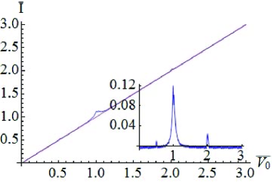
Figure 2: Color online: Dependence of $\bar{I}$ on $\bar{V_{0}}$ in the presence of the nanomagnet (purple) and without the magnet(blue) for $\epsilon=0.1$, $\bar{k}=0.1$, $\bar{\eta}\approx\eta=10^{-4}$, $\omega_{g}/\omega_{R}\ll 1$. The inset shows the difference between the two curves.

In terms of the above variables the equations for $I$ and $m_{z}$ become

$$\bar{I}=\sin(\bar{V}_{0}\bar{t}-\bar{k}\bar{m}_{z})+\frac{\omega_{g}}{\omega_{R}}\left(\bar{V}_{0}-\bar{k}\frac{d\bar{m}_{z}}{d\bar{t}}\right)\,,$$ (25)

$$\frac{d^{2}\bar{m}_{z}}{dt^{2}}+2\tilde{\eta}\frac{d\bar{m}_{z}}{dt}+m_{z}=\epsilon\left(1+\eta\frac{d}{d\bar{t}}\right)\sin(\bar{V}_{0}\bar{t}-\bar{k}\bar{m}_{z})\,.$$ (26)

In these equations the dimensionless parameter $\bar{k}$ can be small or large, depending on the size and the location of the magnet. The ratio ${\omega_{g}}/{\omega_{R}}$ can also be small or large depending on the resistance $R$. The parameter $\epsilon$ roughly equals the ratio of the field created by the critical current at the location of the nanomagnet and the external field. In practical situations this ratio will always be small, thus, justifying the linear approximation for $\bar{m}_{z}$ away from resonance, $\bar{V}_{0}=1$, and at the resonance for not very small $\tilde{\eta}$. In the case of a very narrow resonance (very small $\tilde{\eta}$) one should employ the non-linear approximation based upon the full Landau-Lifshitz equation.

The dependence of $\langle\bar{I}\rangle$ on $\bar{V}_{0}$, computed numerically, is shown in Fig. 2. Shapiro-like steps at $\bar{V}_{0}=1$ and $\bar{V}_{0}=2$ are apparent. They appear due to same physics as the conventional Shapiro steps, with the field of the precessing magnet playing the role of the rf field. The half-Shapiro step that can be seen at $\bar{V}_{0}=0.5$ appears when one solves the full Landau-Lifshitz equation instead of the linearized equation. Fig. 2 illustrates the principal possibility to detect the presence of a small magnet in the vicinity of the weak link by measuring its I-V curve.

IV Non-linear Dynamics and Magnetization Reversal

In this Section we demonstrate the possibility of a reversal of the magnetic moment of the nanomagnet by using a specific time dependence of the bias voltage applied to the weak link. This problem involves a non-linear dynamics described by the full Landau-Lifshitz equation. Consider a nanomagnet with uniaxial magnetic anisotropy

$$K({\bf M})=-\frac{K}{2V}M_{y}^{2}$$ (27)

(with $K$ being a constant and $V$ being the volume of the magnet) in a zero external field. The effective field from this term in the energy is

$${\bf B}_{eff}^{(A)}=\frac{KM_{y}}{V}{\bf e}_{y}\,.$$ (28)

The problem of coupling of the weak link to small oscillations of ${\bf M}$ around ${\bf M}_{0}$ directed along the anisotropy axis becomes identical to the problem studied in the previous section if one replaces $B_{0}$ with $KM_{0}/V$. If both are present $B_{0}$ in the above formulas should be replaced with $B_{0}+KM_{0}/V$.

The dc magnetic field that would be required to switch the magnetic moment to the opposite orientation along the anisotropy axis is $B_{0}=KM_{0}/V$. In all practical situations the magnitude of the oscillating magnetic field produced by the weak link at the location of the magnet will be hopelessly small compared to that field. The question, however, arises whether the ac field produced by the oscillations of the Josephson current can pump spin excitations into the magnet at a rate sufficient to reverse its magnetization. We shall see that this may, indeed, be practicable, thus invoking the possibility of a magnetic memory unit operated by voltage pulses.

When the effective field is dominated by the magnetic anisotropy the roles of the parameters $\omega_{g}$ and $E_{B}$ are played by

$$\omega_{g}=\frac{{\gamma}_{g}KM_{0}}{V}\,,\quad E_{B}=\frac{KM_{0}}{kV}\,.$$ (29)

To simplify our formulas we consider in this Section the limit of a very large normal resistance, so that we can neglect the normal current through the link. (This assumption is unessential for our conclusions, though, and the calculation can easily be generalized to the case when the normal current is present.) Under this assumption the non-linear dynamics of the magnetic moment is described by the dimensionless Landau-Lifshitz equation

$$\frac{\partial\bar{\bf M}}{\partial\bar{t}}=\bar{\bf M}\times\bar{\bf B}_{eff}-{\eta}\bar{\bf M}\times(\bar{\bf M}\times\bar{\bf B}_{eff})$$ (30)

with dimensionless

$$\bar{\bf B}_{eff}=\bar{M}_{y}{\bf e}_{y}+\epsilon\sin(\bar{V}_{0}\bar{t}-\bar{k}\bar{M}_{z}){\bf e}_{z}\,.$$ (31)

Numerical solution of Eq. (30) for a time-linear voltage pulse is shown in Fig. 3.

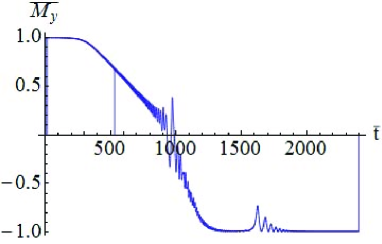
Figure 3: Color online: Reversal of the magnetic moment of the nanomagnet by linearly decreasing bias voltage $\bar{V}=1.5-0.00075\bar{t}$. The values of the parameters are $\epsilon=\bar{k}=0.05$, $\eta=0.01$.

As the effective field decreases in the course of the reversal, the ac field generated by the oscillating tunneling current continuously pumps spin excitations into the nanomagnet. This leads to the full reversal of the magnetic moment. We find numerically that the reversal only occurs at $\epsilon>\eta$. Another observation is that the time needed for the reversal is inversely proportional to $\epsilon$. Practical implications of these findings are discussed in Sec. VI.

V Nanomagnet as a Two-State Quantum System

In this Section we will treat nanomagnet as a fixed-length quantum spin ${\bf S}$, rigidly embedded in a solid matrix. Magnetic anisotropy energy $K({\bf M})$ should now be replaced by a crystal-field Hamiltonian. The general form of such a Hamiltonian that corresponds to a strong easy-axis magnetic anisotropy is

$$\hat{H}_{S}=\hat{H}_{\parallel}+\hat{H}_{\perp}\,,$$ (32)

where $\hat{H}_{\parallel}$ commutes with $S_{z}$ and $\hat{H}_{\perp}$ is a perturbation that does not commute with $S_{z}$. Presence of the magnetic anisotropy axis means that the $|\pm S\rangle$ eigenstates of $S_{z}$ are degenerate ground states of $\hat{H}_{\parallel}$. Operator $\hat{H}_{\perp}$ slightly perturbs the $|\pm S\rangle$ states, adding to them small contributions of other $|m_{S}\rangle$ states. We shall call these degenerate normalized perturbed states $|\psi_{\pm S}\rangle$. Physically they describe the magnetic moment of the nanomagnet looking in one of the two directions along the anisotropy axis. Full perturbation theory with account of the degeneracy of $\hat{H}_{S}$ provides quantum tunneling between the $|\psi_{\pm S}\rangle$ states MQT-book . The ground state and the first excited state are even and odd combinations of $|\psi_{\pm S}\rangle$ respectively,

$$\Psi_{\mp}=\frac{1}{\sqrt{2}}\left(|\psi_{S}\rangle\pm|\psi_{-S}\rangle\right)\,.$$ (33)

They satisfy

$$\hat{H}_{S}\Psi_{\pm}=E_{\pm}\Psi_{\pm}$$ (34)

with

$$E_{+}-E_{-}=\Delta$$ (35)

being the tunnel splitting. The latter is typically small compared to the distance to other spin energy levels, making the two-state approximation rather accurate at low energies. For, e.g., biaxial magnetic anisotropy, $\hat{H}_{S}=-DS_{z}^{2}+dS_{y}^{2}$ with $d\ll D$, the splitting of the lowest energy level appears in the $S$-order on $d/D$, while the distance to the next level equals $(2S-1)D$.

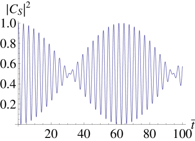
(a) $\;\hbar\omega_{J}=\Delta$

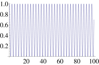
(b) $\;\hbar\omega_{J}=3\Delta/2$

Figure 4: Color online: Rabi oscillations of $|{C}_{S}(\tau)|^{2}$ at ${2\bar{k}E_{J}}/{\Delta}=0.1$ for two constant voltages with the initial condition ${C}_{S}(0)=1$.

Since the two low-energy spin states of quantum nanomagnet are superpositions of $|\psi_{\pm S}\rangle$, it is convenient to describe such a two-state system by a pseudospin 1/2. Components of the corresponding Pauli operator ${\bm{\sigma}}$ are

$$\sigma_{x} = |\psi_{-S}\rangle\langle\psi_{S}|+|\psi_{S}\rangle\langle\psi_{-S}|$$

$$\sigma_{y} = i|\psi_{-S}\rangle\langle\psi_{S}|-i|\psi_{S}\rangle\langle\psi_{-S}|$$

$$\sigma_{z} = |\psi_{S}\rangle\langle\psi_{S}|-|\psi_{-S}\rangle\langle\psi_{-S}|\,.$$ (36)

The projection of any operator $\hat{A}_{S}=\hat{A}(\hat{\bf S})$ onto $|\psi_{\pm S}\rangle$ states is

$$\hat{A}_{\sigma}=\sum_{m,n=\psi_{\pm S}}\langle m|\hat{A}_{S}|n\rangle|m\rangle\langle n|\,.$$ (37)

Expressing $|\psi_{\pm S}\rangle$ via $\Psi_{\pm}$ according to Eq. (33), it is easy to see from Eq. (34) that

$$\langle\psi_{\pm S}|\hat{H}_{S}|\psi_{\pm S}\rangle=0,\quad\langle\psi_{-S}|\hat{H}_{S}|\psi_{S}\rangle=-{\Delta}/{2}\,.$$ (38)

With the help of these relations one obtains from Eq. (37)

$$\hat{H}_{\sigma}^{(S)}=-({\Delta}/{2})\sigma_{x}\,.$$ (39)

Quantum generalization of Eq. (2) with account of Eqs. (6) and (18) is

$$\hat{H}_{J}=-E_{J}\cos(\omega_{J}t-k\mu_{B}\hat{S}_{z})\,.$$ (40)

Equations (V) and (37) then give

$$\hat{H}_{\sigma}^{(J)}=-E_{J}[\cos(\omega_{J}t)+k\mu_{B}S\sigma_{z}\sin(\omega_{J}t)]\,,$$ (41)

where

$$\omega_{J}(t)=\frac{2e}{\hbar}V_{0}(t)\,.$$ (42)

The total Hamiltonian of our two-level system is

$$\hat{H}_{\sigma}=-{\bf b}_{eff}\cdot{\bm{\sigma}}\,,$$ (43)

where

$$\hat{\bf b}_{eff}=({\Delta}/{2}){\bf e}_{x}+\bar{k}E_{J}\sin(\omega_{J}t){\bf e}_{z}\,.$$ (44)

Here, as before, $\bar{k}=kM_{0}=k\mu_{B}S$, so that the energy $\bar{k}E_{J}$ roughly represents the strength of the interaction of the magnetic flux of the junction with the spin ${\bf S}$. In practice this interaction can be greater or smaller than $\Delta$.

The above system represents a simple realization of the spin qubit proposed by Nazarov Nazarov-2010 . Quantum states of such a qubit are described by the wave function

$$\Psi=C_{S}|\psi_{S}\rangle+C_{-S}|\psi_{-S}\rangle\,.$$ (45)

The Schrödinger equation for $|\Psi\rangle$ is

$$i\hbar\frac{d\Psi}{dt}=\hat{H}_{\sigma}\Psi\,.$$ (46)

Here $|C_{\pm S}|^{2}$ is the probability for the spin to look up or down along the $z$-direction, with $|C_{+S}|^{2}+|C_{-S}|^{2}=1$. Introducing

$$\tilde{C}_{\pm S}(t)=C_{\pm S}(t)\exp\left\{\frac{i\bar{k}E_{J}}{2\hbar}\int_{t_{0}}^{t}dt^{\prime}sin[\omega_{J}(t^{\prime})t^{\prime}]\right\}\,,$$ (47)

we obtain from Eq. (46)

$$i\hbar\frac{d}{dt}\tilde{C}_{-S} =\frac{\Delta}{2}\tilde{C}_{S}$$

$$i\hbar\frac{d}{dt}\tilde{C}_{S}= -\bar{k}E_{J}\tilde{C}_{S}\sin(\omega_{J}t)+\frac{\Delta}{2}\tilde{C}_{-S}\,.$$ (48)

In terms of dimensionless time, $\bar{t}={\Delta t}/({2\hbar})$, the resulting equation for $\tilde{C}_{S}$ is

$$\frac{d^{2}}{d{\bar{t}}^{2}}\tilde{C}_{S}-i\frac{2\bar{k}E_{J}}{\Delta}\frac{d}{d\bar{t}}\left[\sin\left(\frac{2\hbar\omega_{J}}{\Delta}\bar{t}\right)\tilde{C}_{S}\right]+\tilde{C}_{S}=0$$ (49)

The effect of the bias voltage becomes especially pronounced at $V_{0}$ satisfying $\omega_{J}=(m/n)\Delta$, where $m$ and $n$ are integers. Fig. 4 shows Rabi oscillations of the probability to remain in the initial spin-up state for two different bias voltages each satisfying one of the above conditions.

VI Discussion

We have studied electromagnetic interaction between a weak superconducting link and a small magnet placed in the vicinity of the link. Three problems have been considered: Shapiro-like steps in the I-V curve generated by the magnet, the reversal of the magnetic moment by a time-dependent bias voltage, and Rabi oscillations of the quantum spin induced by a constant voltage.

For the first two problems the strength of the interaction is determined by the parameter $\epsilon={E_{J}}/{E_{B}}$. By order of magnitude ${\epsilon}$ represents the ratio of the magnetic field generated by the tunneling current and the effective field, $B_{eff}$, acting on the magnetic moment due to magnetic anisotropy and the applied external field. We show that precession of the magnetic moment generates Shapiro-like steps in the I-V curve of the superconducting weak link. The possibility to observe the first Shapiro step at $\bar{V}_{0}=1$ (and also the peak at $V_{0}=0.5$ due to non-linearity) appears quite realistic. Note that the first step scales down linearly with $\epsilon$ when decreasing $\epsilon$, the second step at $\bar{V}_{0}=2$ scales as $\epsilon^{2}$, and so on. Thus, for small $\epsilon$, higher steps may be more difficult to see in experiment.

A remarkable observation is that despite the weakness of the field generated by the tunneling current of the link, for a certain time dependence of the bias voltage it can effectively pump spin excitations into the magnet, leading to the reversal of its magnetic moment. The damping constant $\eta=0.01$ was chosen for simulations of the reversal. This value is realistic for magnetic nanoparticles Coffey-1998 . We find that condition $\epsilon>\eta$ is required for the reversal, which must be important for experiment. The parameter $\epsilon$ determines the number of cycles in the precession of the magnetic moment that leads to the reversal of the moment. In our numerical simulations that number roughly scaled as $1/\epsilon$. For $\epsilon=0.05$ used to obtain the plot shown in Fig. 3 the time required to reverse the moment was close to $10^{3}\omega_{g}^{-1}$. For, e.g., $\omega_{g}\sim 10^{11}$s^-1 this would provide a reversal in ten nanoseconds. The linear time dependence of the bias voltage in Fig. 3 was chosen to maintain the condition of continuous pumping of spin excitations into the magnet. Smaller $\epsilon$ would require slower time dependence of $V_{0}$, which should not be difficult to satisfy in experiment. However, smaller $\epsilon$ would require smaller $\eta$ due to the condition $\epsilon>\eta$. Also, the smaller is $\epsilon$ the more sensitive the time evolution of the magnetic moment becomes to the time dependence of the voltage. A slight change in that dependence is sufficient for the moment to bounce back to the initial direction after reaching the top of the anisotropy barrier.

In the quantum problem, the parameter $\epsilon$ is no longer relevant. The relevant parameter becomes the ratio of the Zeeman interaction of the spin with the field of the tunneling current and the tunnel splitting $\Delta$. This parameter can be small or large depending on the splitting. Rabi oscillations of the spin are strongly affected by the bias voltage. The most noticeable effect appears at $V_{0}$ satisfying one of the resonant conditions $eV_{0}=(m/n)\Delta$, where $m$ and $n$ are integers. At such resonances the behavior of the probability to find the spin in up or down configurations is very different from the off-resonance behavior. This demonstrates the principal possibility to electromagnetically manipulate a nanomagnet - weak link qubit by the voltage applied to the link.

VII Acknowledgements

The authors acknowledge invaluable discussions with Wolfgang Wernsdorfer. This work has been supported by the U.S. Department of Energy through Grant No. DE-FG02-93ER45487.

References

- (1) C. Bell, S. Milikisyants, M. Huber, and J. Aarts, Phys. Rev. Lett. 100, 047002 (2008).
- (2) See, e.g., review: A. I. Buzdin, Rev. Mod. Phys. 77, 935 (2005).
- (3) A. Buzdin, Phys. Rev. Lett. 101, 107005 (2008).
- (4) F. Konschelle and A. Buzdin, Phys. Rev. Lett. 102, 017001 (2009).
- (5) M. Houzet, Phys. Rev. Lett. 101, 057009 (2008).
- (6) I. Petković, M. Aprili, S. E. Barnes, F. Beuneu, and S. Maekawa, Phys. Rev. B 80, 220502(R) (2009).
- (7) I. O. Kulik, Sov. Phys. JETP 22, 841 (1966).
- (8) L. N. Bulaevskii, V. V. Kuzii, and A. A. Sobyanin, JETP Lett. 25, 290 (1977).
- (9) J.-X. Zhu, Z. Nussinov, A. Shnirman, and A.V. Balatsky, Phys. Rev. Lett. 92, 107001 (2004).
- (10) Z. Nussinov, A. Shnirman, D. P. Arovas, A. V. Balatsky, and J. X. Zhu, Phys. Rev. B 71, 214520 (2005).
- (11) L. Dell Anna, A. Zazunov, R. Egger, and T. Martin, Phys. Rev B 75, 085305 (2007).
- (12) S. K. H. Lam, W. Yang, H. T. R. Wiogo, and C. P. Foley, Nanotechnology 19, 285303 (2008).
- (13) C. Benjamin, T. Jonckheere, A. Zazunov, and T. Martin, Eur. Phys. J. B, 57 279 (2007); M. Lee, T. Jonckheere, and T. Martin, Phys. Rev. Lett. 101, 146804 (2008).
- (14) S. Teber, C. Holmqvist, M. Fogelstrom, Physical Review B 81, 174503 (2010).
- (15) A. V. Samokhvalov, Phys. Rev. B 80, 134513 (2009).
- (16) C. Padurariu and Yu. V. Nazarov, Phys. Rev. B 81, 144519 (2010).
- (17) Y. M. Galperin, D. V. Shantsev, J. Bergli, B. L. Altshuler, Europhys. Lett. 71, 21 (2005); I. Martin, L. Bulaevskii, and A. Shnirman, Phys. Rev. Lett. 95, 127002 (2005); L.-C. Ku and C. C. Yu, Phys. Rev. B 72, 024526 (2005); A. M. Zagoskin, S. Ashhab, J. R. Johansson, and F. Nori, Phys. Rev. Lett. 97, 077001 (2006).
- (18) W. Wernsdorfer, Adv. Chem. Phys. 118, 99 (2001).
- (19) W. Wernsdorfer, Superconductor Science & Technology 22, 064013 (2008).
- (20) C. Thirion, W. Wernsdorfer, and D. Mailly, Nature Materials 2, 524 (2003).
- (21) E. M. Chudnovsky and J. Tejada, Lectures on Magnetism (Rinton Press, Princeton, NJ, 2008).
- (22) J.-P. Cleuziou, W. Wernsdorfer, V. Bouchiat, T. Ondarcuhu, and M. Monthioux, Nature Nanotechnology 1, 53 (2006); J.-P. Cleuziou, W. Wernsdorfer, S. Andergassen, S. Florens, V. Bouchiat, T. Ondarcuhu, and M. Monthioux, Phys. Rev. Lett. 99, 117001 (2007); L. Bogani, R. Maurand, L. Marty, C. Sangregorio, C. Altavillad, and W. Wernsdorfer, J. Mater. Chem. 20, 2099 (2010).
- (23) M. Faucher, P.-O. Jubert, O. Fruchart, W. Wernsdorfer, V. Bouchiat, Superconductor Science & Technology 22, 064010 (2009).
- (24) L. Bogani and W. Wernsdorfer, Nature Materials 7, 179 (2008).
- (25) The concept of quantum computing with qubits formed by nanomagnets inside Josephson junctions has also been proposed in J. Tejada, E. M. Chudnovsky, E. del Barco, J. M. Hernandez, and T. P. Spiller, Nanotechnology 12, 181 (2001).
- (26) E. M. Chudnovsky and J. Tejada, Macroscopic Quantum Tunneling of the Magnetic Moment (Cambridge University Press, Cambridge, UK, 1998).
- (27) W. T. Coffey, D. S. F. Crothers, J. L. Dormann, Y. P. Kalmykov, E. C. Kennedy, and W. Wernsdorfer, Phys. Rev. Lett. 80, 5655 (1998).