Stochastic heating of a molecular nanomagnet

Abstract

We study the excitation dynamics of a single molecular nanomagnet by static and pulsed magnetic fields. Based on a stability analysis of the classical magnetization dynamics we identify analytically the fields parameters for which the energy is stochastically pumped into the system in which case the magnetization undergoes diffusively and irreversibly a large angle deflection. An approximate analytical expression for the diffusion constant in terms of the fields parameters is given and assessed by full numerical calculations.

I Introduction

In molecular nanomagnets (MNMs) MM such as in Mn₁₂ acetates the magnetic core of the molecule is surrounded by organic non-magnetic ligands that extinguish the inter MNM exchange interactions. Hence, much of the on-site physical properties are deducible by studying a single MNM, albeit the dipolar interaction is present and is essential for ordering phenomena garanin . Characteristic for MNMs is the relatively large effective spin (e.g., $S$ = 16 for Mn₁₂) and the magnetic anisotropy MM . MNMs exhibit a series of phenomena MM that are relevant for applications in spintronics and quantum information Mabuchi ; most notably is the bistability behaviour, the resonance tunneling of magnetization Chudnovsky and the large spin relaxation time. The dynamical control and switching of the magnetization via external fields is a key ingredient on the way to utilizing MNM for technological applications. In this context, the role of thermal and environmental effects have been considered Khapikov ; Denisov . For a single MNM Lis ; Quantum ; Friedman ; Hernandez ; Lionti ; Chudnovsky ; Thomas ; Wernsdorfer ; Hennion at very low temperatures the main switching mechanism is the quantum tunneling of magnetization Quantum . This is due to the large anisotropy barrier Gatteschi . For an initially excited MNM and driven by external magnetic fields we have shown recently Chotorlishvili that the phase space of the magnetization has a rich structure containing a separatrix of topologically different domains. Switching occurs at the separatrix as a consequence of a transition between these domains. However, the issue how to inject energy in this nonlinear system, i.e. how to realize the initially excited state near the separatrix, has not been addressed. Starting from the ground state, this question is not answered by resonant fields as the system is non-linear, i.e. it changes its eigenfrequency as the oscillation amplitude varies Chotorlishvili . Formally the equations of motion for a single molecular magnet resembles the Landau-Lifshitz-(Gilbert) equation without the Gilbert damping. In the present case the negligible damping is an inherent system property and not a shortcoming of theory. This difference is insofar important as without dissipation a precessional switching, e.g. as proposed in Bauer , is not achievable. Hence, new switching schemes are needed for MNM that are different from those known for magnetic materials. One scheme proposed recently Chotorlishvili relies on a stochastic, diffusion-type switching. For this to work however, the system has to be excited to a desired state (near the separatrix). The question of how to achieve that is still open. In this paper we show that using appropriate polychromatic magnetic pulses we can achieve a stochastic heating of a molecular magnet as appropriate for the stochastic switching. We derive approximate analytical expressions for the field parameters that allow for the stochastic heating and test for our analytical predictions with full numerical calculations.

II Theoretical model

We study a single molecular magnet (MM), e.g. Fe₈ or Mn₁₂ acetates and choose the $z$ axis to be along the uniaxial anisotropy direction (easy axis). The MM is subjected to a constant magnetic field with an amplitude $H_{0}$, applied along the $x$-axis (hard axis) as well as to a series of magnetic pulses ${\cal F}(t)$ that are linearly polarized in the $x$ direction. The Hamiltonian we write as Chotorlishvili :

$$\hat{H}=\hat{H}_{0}+\hat{H}_{I},$$ (1)

$$\hat{H}_{0}=-D\hat{S}_{z}^{2}+g\mu_{B}H_{0}\hat{S}_{x},\hat{H}_{I}=g\mu_{B}{\cal F}(t)\hat{S}_{x}.$$

Here $D$ is the longitudinal anisotropy constant, $S_{x}$, $S_{y}$, and $S_{z}$ are the spin operators projections along the $x,y$, and $z$ directions, respectively. $g$ is the Landé factor, and $\mu_{B}$ is the Bohr magneton. Since the spin of the molecular nanomagnet is quite large a classical approximation is appropriate. Hence, it is advantageous to introduce the variables $(S_{z},~{}\varphi)$ via the transformation

$$S_{x}=\sqrt{1-S_{z}^{2}}\cos\varphi,\;S_{y}=\sqrt{1-S_{z}^{2}}\sin\varphi$$

and rewrite (1) in the compact form Chotorlishvili

$$H(t) = -\frac{\lambda}{2}S_{z}^{2}+\sqrt{1-S_{z}^{2}}\cos\varphi-\sqrt{1-S_{z}^{2}}\cos\varphi F(t)$$

$$\lambda = \frac{2DS}{g\mu_{B}H_{0}},\>F(t)=\frac{{\cal F}(t)}{g\mu_{B}H_{0}}.$$ (2)

Suppose that the applied constant field is weak $\lambda>1$ and at the initial moment of time the system resides near to the ground state $S_{z}(t=0)\approx\pm 1$. How to pump efficiently energy into the system such that we reach the excited states near the separatrix, where then a dynamically induced switching is realizable? To answer this question we make a transition to the action-angle variables $(I,\varphi)$ in which the Hamiltonian (II) reads

$$H=H_{0}(I)+V(I,\varphi)F(t),$$

$$H_{0}=\omega(I)I,\omega(I)=\bigg{[}\frac{dI(\Sigma)}{d\Sigma}\bigg{]}^{-1},$$ (3)

$$I(\Sigma)=\frac{1}{\pi}\int S_{z}(\Sigma,\varphi)d\varphi,~{}~{}~{}~{}\Sigma=-H.$$

The equations of motion (EOM) are

$$\dot{I}=-\frac{\partial H}{\partial\varphi}=-\frac{\partial V(I,\varphi)}{\partial\varphi}F(t),$$

$$\dot{\varphi}=\frac{\partial H}{\partial I}=\omega(I)+\frac{\partial V(I,\varphi)}{\partial I}F(t).$$ (4)

In absence of the time dependent perturbation, $I$ is an integral of motion ($\varphi(t)$ is fast variable, however). For an applied monochromatic field it is not possible to keep in resonance with $\omega$, for $\omega$ depends on $I$ and hence it changes in time. A polychromatic field offers a wider range of frequencies that may match the dynamical frequency of the system. To be more concrete let us assume the applied field to be of the form

$$F=\varepsilon_{0}T\sum\limits_{n=-\infty}^{\infty}\delta_{\tau}(t-nT)=\varepsilon_{0}\frac{\tau}{T}\sum\limits_{n=-1/\tau}^{1/\tau}\cos\bigg{(}\frac{2\pi}{T}nt\bigg{)},$$ (5)

where $\tau$ is the pulse duration, $T>\tau$ is interval between pulses, and $\varepsilon_{0}$ is the pulse strength.

III Stochastic heating

Of particular interest for us is the situation of overlapping resonances which is realized when Zaslavsky

$$K^{\prime}=\varepsilon_{0}TI(\Sigma)\frac{d\omega(I)}{dI(\Sigma)}>1,$$ (6)

in which case the dynamics turns chaotic Zaslavsky , i.e. the system jumps from one resonance to other in a random way. A key point here is the irreversibility of the dynamics that emerges due to nonlinearity and without any thermal effects nor external random forces. Hence, we expect a ”stochastic heating” of a MM subjected to the pulses (5) when the criterion (6) is fulfilled.

Assuming that $S_{z}(t=0)\approx\mp 1$ and $\lambda>1$ we find

$$I(\Sigma)=\int S_{z}(\Sigma,\varphi)d\varphi=\frac{2}{\sqrt{\lambda}}\sqrt{\Sigma-1}E\Big{(}\frac{2}{\Sigma-1}\Big{)},$$

$$\omega(I)=\bigg{[}\frac{dI(\Sigma)}{d\Sigma}\bigg{]}^{-1}=\frac{\sqrt{\lambda}\sqrt{\Sigma-1}}{K\big{(}\frac{2}{\Sigma-1}\big{)}},$$ (7)

$$\frac{d\omega(I)}{dI}=\frac{d\omega(I)}{d\Sigma}\frac{d\Sigma}{dI}=\omega(I)\frac{d\omega(I)}{d\Sigma},$$

$$\frac{d\omega(I)}{d\Sigma}=\frac{\sqrt{\lambda}\sqrt{\Sigma-1}E\big{(}\frac{2}{\Sigma-1}\big{)}}{2(\Sigma-3)K^{2}\big{(}\frac{2}{\Sigma-1}\big{)}}.$$

Thus we infer

$$K^{\prime}=\varepsilon_{0}T\frac{\sqrt{\lambda}(\Sigma-1)^{3/2}E^{2}\big{(}\frac{2}{\Sigma-1}\big{)}}{(\Sigma-3)K^{3}\big{(}\frac{2}{\Sigma-1}\big{)}}>1.$$ (8)

$E\big{(}\frac{2}{\Sigma-1}\big{)}$, $K\big{(}\frac{2}{\Sigma-1}\big{)}$ are the complete elliptic integrals in the notation of Ref.[Handbook, ]. In the regime of chaotic motion, when Eq.(6) holds, a dynamical description becomes inappropriate. The adequate language for the study of the magnetization dynamics in this case is an approach based for example on the Fokker-Planck equation. A Fokker-Planck equation for the distribution function of the action $f(I,t)$ can be set up in a similar way as done in Ref.[Toklikishvili, ]:

$$\frac{\partial f(I,t)}{\partial t}=\frac{1}{2}\frac{\partial}{\partial I}D(I)\frac{\partial f(I,t)}{\partial I},\,D(I)=\frac{\varepsilon^{2}T}{2}\big{(}1-\frac{2}{\lambda}I\omega(I)\big{)}.$$

The relevant quantity is the averaged value of the action $\langle I(t,\Sigma)\rangle_{f}=\overline{I(t)}.$ Using the relations

$$\int I\frac{\partial f(I,t)}{\partial t}dI=\frac{1}{2}\int I\frac{\partial}{\partial I}D(I)\frac{\partial f(I,t)}{\partial I}dI,$$ (9)

$$\dot{\bar{I}}(t)=-\frac{1}{2}\int D(I)\frac{\partial f(I,t)}{\partial I}dI=\frac{1}{2}\int\frac{\partial D(I)}{\partial I}f(I,t)dI,$$ (10)

$$\frac{\partial D(I)}{\partial I}=-\frac{\varepsilon^{2}_{0}T}{2\lambda}\omega(I)\bigg{(}1+I\frac{d\omega(I)}{d\Sigma}\bigg{)},$$ (11)

we infer that

$$\dot{\bar{I}}=-\frac{\varepsilon^{2}_{0}T}{2\lambda}\omega(\bar{I})\bigg{(}1+\bar{I}\frac{d\omega(\bar{I})}{d\Sigma}\bigg{)}.$$ (12)

We note that $I$ and $\omega(I)$ are functions of $\Sigma$ and make the approximation that

$$\bar{I}(\Sigma)=I(\bar{\Sigma}),~{}~{}~{}\bar{\omega}(I)=\bar{\omega}\big{(}I(\bar{\Sigma})\big{)},$$ (13)

meaning that correlations between the random variables are neglected. Formally, we can systematically improve on this approximation by accounting for higher moments for the correlation functions of the random variables. Neglecting these correlations we find for $\dot{\bar{I}}$

$$\dot{\bar{I}}=\overline{\frac{dI}{d\Sigma}\frac{d\Sigma}{dt}}=-\frac{\varepsilon^{2}_{0}T}{2\lambda}\omega(\bar{I})\bigg{(}1+\bar{I}\frac{d\omega(\bar{I})}{d\Sigma}\bigg{)},$$ (14)

$$\overline{\frac{d\Sigma}{dt}}=-\frac{\varepsilon^{2}_{0}T}{\lambda}\omega^{2}(\bar{I})\bigg{(}1+\bar{I}\frac{d\omega(\bar{I})}{d\Sigma}\bigg{)}$$ (15)

we conclude that

$$\frac{d\overline{\Sigma}}{dt}=-\varepsilon^{2}_{0}T\frac{\overline{\Sigma}-1}{K^{2}(\frac{2}{\overline{\Sigma}-1})}\Bigg{(}1+\frac{\overline{\Sigma}-1}{\overline{\Sigma}-3}\frac{E^{2}(\frac{2}{\overline{\Sigma}-1})}{K^{2}(\frac{2}{\overline{\Sigma}-1})}\Bigg{)}.$$ (16)

¿From the asymptotical solution of $\bar{\Sigma}>1$

$$\bar{\Sigma}(t)=\frac{\lambda}{2}\exp\bigg{[}-\frac{4}{\pi}\varepsilon^{2}_{0}Tt\bigg{]}$$ (17)

we uncover a diffusive decay of $\bar{\Sigma}(t)$, meaning that the energy is increased diffusively due to the relation $H=-\bar{\Sigma}(t)$), albeit eq. (8) must be obeyed.

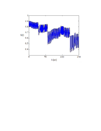
Figure 1: A demonstration of the stochastic deflection of the magnetization vector from the initial state $S_{z}(0)=0.9$ upon applying a series of rectangular pulses. The results are obtained by solving numerically for the Hamiltonian equations. The time scale is set by values of the constant magnetic field $t\rightarrow t/g\mu_{B}H_{0}$ [16]. The parameters are $\varepsilon_{0}=0.4$, $T=1ps$, $\tau=0.01ps$, $\lambda=10$. Note, the criterion of the stochasticity, given by (8) is realized since $K^{\prime}=1.75>1$.

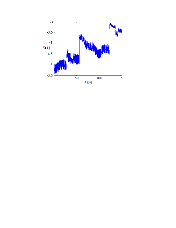
Figure 2: Illustration of the stochastic heating by external driving fields after having started from the initial state $S_{z}(0)=0.9$. The results are obtained as in Fig. 1 with the parameters $\varepsilon_{0}=0.4$, $T=1ps$, $\tau=0.01ps$, $\lambda=10$. The criterion of stochasticity (8) is fulfilled ($K^{\prime}=1.75>1$) and a diffusive increase of the system energy is observed. This numerical result is qualitatively consistent with the analytical prediction, given by Eq. (17). For a better numerical agreement one has to go beyond the approximation (13) and consider higher moments for the correlation functions of the random variables

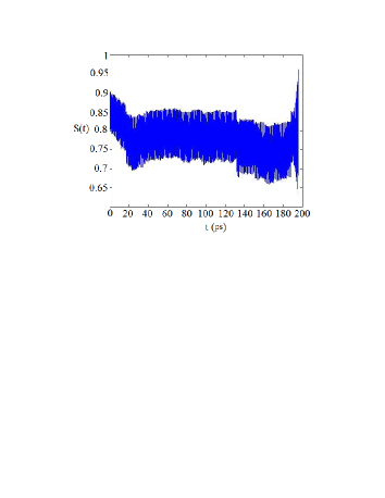
Figure 3: The time evolution of the magnetization vector when starting from the initial state $S_{z}(0)=0.9$. The results are obtained by solving numerically for the Hamiltonian equations with a series of rectangular pulses. The parameters are $\varepsilon_{0}=0.1$, $T=1ps$, $\tau=0.01ps$, $\lambda=10$, $K^{\prime}=0.43<1$. The criterion of stochasticity is not fulfilled. The orientation of the magnetic vector is not changed significantly, and only fluctuations around the ground state is observed.

IV Numerical results

The exact numerical results shown in Figs.(1, 2, 3) evidence that the mechanism of stochastic heating is indeed present and is quite efficient.

Other scenario for the magnetization control is to employ only the periodic series of rectangular pulses applied along the hard axis, i.e. to switch off the static field. Measuring the energy in units of $D$ we write for the scaled Hamiltonian

$$\bar{H}(t)={H}(t)/D=-\frac{S_{z}^{2}}{2}+V(s_{z},\varphi),$$

where

$$V(s_{z},\varphi)=V_{0}(s_{z},\varphi)\,T\sum\limits_{k=-\infty}^{+\infty}\delta(t-kT),$$

and

$$V_{0}(s_{z},\varphi)=\varepsilon\sqrt{1-s_{z}^{2}}\cos\varphi,$$

with

$$\varepsilon=\frac{\varepsilon_{0}}{D}.$$

The equations of motion

$$\dot{\varphi}=\omega(s_{z})+\varepsilon\frac{\partial V_{0}(s_{z},\varphi)}{\partial s_{z}}T\,\sum\limits_{k=-\infty}^{+\infty}\delta(t-kT),$$ (18)

$$\dot{s}_{z}=-\varepsilon\frac{\partial V_{0}(s_{z},\varphi)}{\partial\varphi}T\,\sum\limits_{k=-\infty}^{+\infty}\delta(t-kT),\,\omega(s_{z})=-s_{z}$$

can be integrated exactly in this case by formulating them as recurrence relations Zaslavsky using the evolution operator $\hat{T}$ that propagate the system from the time $t_{0}$ to $T$, i.e.

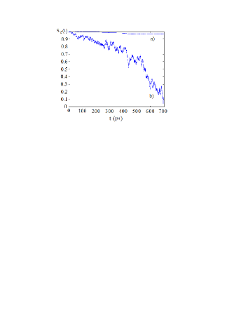
Figure 4: $S_{n}^{z}(t)$ as a function of the number of applied kicks $t=nT$ obtained from a full numerical integration of the recurrence relations eq.(19). The basic control parameter is the time interval between the pulses $T$ which allows a tuning of the values of of stochasticity coefficient (because $D_{diff}=\frac{1}{4}(\frac{\varepsilon_{0}}{D})^{2}T$) and hence allows a realization of different types of dynamics. We consider the following initial conditions for (19): a) $\varepsilon=0.1$,   $S_{z}(0)=0.99,~{}~{}\varphi(0)=0$,   $T=0.01ps$, and $K_{0}=10^{-5}$. b) $\varepsilon=0.1$,   $S_{z}(0)=0.99,~{}~{}\varphi(0)=0$,   $T=0.1ps$, and $K_{0}=10^{-3}$.

$$(\overline{s_{z}},\overline{\varphi})=\hat{T}(s_{z},\varphi),\overline{s_{z}}=s_{z}(t_{0}+T-0),$$

$$\overline{\varphi}=\varphi(t_{0}+T-0),\,s_{z}=s_{z}(t_{0}-0),\,\varphi=\varphi(t_{0}-0).$$

Note, that $\hat{T}=\hat{T}_{R}\,\hat{T}_{\delta}$ consists of two parts, one describing the free rotations $\hat{T}_{R}$ and the other, $\hat{T}_{\delta}$, the action of the applied pulses, i.e.

$$\hat{T}_{R}(s_{z};\varphi)=(s_{z};\varphi+\omega(s_{z})T).$$

For $\hat{T}_{\delta}$ we find upon integrating EOM

$$\hat{T}_{\delta}(s_{z},\varphi)=\bigg{(}s_{z}-\varepsilon\frac{\partial V_{0}(s_{z},\varphi)}{\partial\varphi},\varphi+\varepsilon T\frac{\partial V_{0}(s_{z},\varphi)}{\partial\varphi}\bigg{)}.$$

Thus the recurrence relation applies

$$\bar{s_{z}}=s_{z}-\varepsilon T\sqrt{1-s_{z}^{2}}\sin\varphi,$$ (19)

$$\bar{\varphi}_{n}=\varphi_{n}-s_{z}T+\varepsilon T^{2}\sqrt{1-s_{z}^{2}}\sin\varphi+\frac{\varepsilon Ts_{z}}{\sqrt{1-s_{z}^{2}}}\cos\varphi.$$

Depending on the chosen parameters, these relations (19) may be be stable or unstable as signified by the corresponding Lyapunov exponents. Here, we inspect the Jacobean matrix

$$M=\frac{\partial(\overline{s_{z}},\overline{\varphi})}{\partial(s_{z},\varphi)}=\left(\begin{array}[]{c}\frac{\partial\overline{s_{z}}}{\partial s_{z}}~{}~{}~{}\frac{\partial\overline{s_{z}}}{\partial\varphi}\\ \frac{\partial\overline{\varphi}}{\partial s_{z}}~{}~{}~{}\frac{\partial\overline{\varphi}}{\partial\varphi}\end{array}\right)$$

and find for the eigenvalues

$$\lambda_{1,2}=1+\frac{1}{2}K\pm\sqrt{(1+\frac{1}{2}K)^{2}-1},$$

$$K=\varepsilon T^{2}\frac{\partial^{2}V_{0}}{\partial\varphi^{2}}=\varepsilon T^{2}\sqrt{1-s_{z}^{2}}\cos\varphi=K_{0}\sqrt{1-s_{z}^{2}}\cos\varphi,$$

where $K_{0}=maxK=\varepsilon T^{2}.$ Chaos is expected if $\lambda_{1}>1$, i.e. for $K>0$, meaning even weak pulses $K_{0}=\varepsilon T^{2}>0$ may lead to a diffusion. I.e., $S_{n}^{z}(t)=S^{z}(t=nT)$ and the magnetization can be deflected diffusively and irreversibly if $K_{0}$ exceeds a critical value $K_{0}^{\prime}$, as demonstrated by the numerical calculations in Fig.3. Essential for this phenomena is the existence of two time scales, the slow variables $S_{n}^{z}(t)$ and the fast random phase $\varphi(t)$. Using the random phase approximation for the fast phases Toklikishvili one infers the Fokker-Planck equation

$$\frac{\partial f(s_{z},t)}{\partial t}=\frac{1}{2}\frac{\partial}{\partial s_{z}}D(s_{z})\frac{\partial f(s_{z},t)}{\partial s_{z}},$$

where

$$D(s_{z})=\frac{\pi\varepsilon^{2}}{\Omega}\sum\limits_{m=-\infty}^{+\infty}m^{2}|V_{m}(s_{z})|^{2}~{}\Omega=\frac{2\pi}{T};$$

and $V_{m}(s_{z})$ are the Fourier coefficients as deduced from the expansion

$$V_{0}(s_{z},\varphi)=\sum\limits_{n=-\infty}^{+\infty}V_{m}(s_{z})\exp(in\varphi).$$

Explicitly we have

$$V_{0}(s_{z},\varphi)=-\sqrt{1-s_{z}^{2}}\cos\varphi=\frac{\sqrt{1-s_{z}^{2}}}{2}(e^{i\varphi}+e^{-i\varphi}).$$

Therefore,

$$V_{1}=V_{-1}=-\frac{\sqrt{1-s_{z}^{2}}}{2},$$

and the diffusion coefficient is

$$D(s_{z})=\frac{\pi\varepsilon^{2}}{\Omega}(|V_{-1}|^{2}+|V_{1}|^{2})=\frac{\pi\varepsilon^{2}}{2\Omega}(1-s_{z}^{2})=\frac{\varepsilon^{2}T}{4}(1-s_{z}^{2}).$$

Consequently, we write

$$\frac{\partial f(s_{z},t)}{\partial t}=D_{diff}\frac{\partial}{\partial s_{z}}(1-s_{z}^{2})\frac{\partial f(s_{z},t)}{\partial s_{z}},$$

where

$$D_{diff}=\frac{\varepsilon^{2}T}{4}$$

is the coefficient of diffusion which is completely defined by the pulse parameters

$$\frac{d}{dt}\langle S_{z}\rangle=-2D\langle S_{z}\rangle,\,\langle S_{z}\rangle=\int\limits_{-1}^{+1}S_{z}f(S_{z},t)dS_{z}.$$ (20)

Thus, the mean value of the spin projection behaves as

$$\langle S_{z}(t)\rangle=\langle S_{z}(0)\rangle e^{-2D_{diff}t}.$$

Since the diffusion coefficient is given by

$$D_{diff}=\frac{\varepsilon^{2}T}{4}=\frac{1}{4}\left(\frac{\varepsilon_{0}}{D}\right)^{2}T$$

($D$ is the magnetic anisotropy constant) $D_{diff}$ can be tuned by changing appropriately the external field parameters, e.g. by varying the amplitude of the pulses $\varepsilon_{0}$ and/or the interval $T$ between them. Depending on these parameters different types of the dynamics is realized. To test for this analytical prediction we performed full numerical calculations that are in good accord with the analytical results (see Fig.4). This statement is based on the fact that for $\varepsilon=0.1,~{}T=0.1,~{}D_{diff}=\varepsilon^{2}T=0.001$ the analytically estimated decay rate $1/D_{diff}$ coincides with the numerically deduced one (cf. Fig.4).

V Summary

The aim of this work is to point out the possibility of a stochastic energy pumping and magnetization deflection in a single molecular magnet subjected to a static and a time-variable, polychromatic magnetic fields. The key point is that the parameters of the applied static and pulsed magnetic fields can be tuned such that the system is driven nearby a separatrix where the magnetization dynamics turns diffusive allowing thus for a magnetization switching even in the absence of damping (that conventionally originates from coupling to other degrees of freedom).

Acknowledgment: The project is supported by the Georgian National Foundation (grants: GNSF/STO 7/4-197, GNSF/STO 7/4-179) and by the Deutsche Forschungsgemeinschaft (DFG) through SFB 762 and through SPP 1285.

References

• (1) Single-Molecule Magnets and Related Phenomena. Structure and Bonding, Ed. R. Winpenny (Springer, Berlin, 2006).
• (2) D. A. Garanin, E. M. Chudnovsky, Phys. Rev. B 78, 174425 (2008).
• (3) H. Mabuchi, A. Doherty, Science 298, 1372 (2002); C.J. Hood et al., Science 287, 1447 (2000); J. Raimond, M. Brune, S. Haroche, Rev. Mod. Phys. 73, 565 (2001).
• (4) E. M. Chudnovsky and J. Tajida, Macroscopic Quantum Tunneling of the Magnetic Moment (Cambridge University Press, Cambrige, England, 1998).
• (5) A. Khapikov and L. Uspenskaya, Phys. Rev. B 74, 14990 (2006); A. Khapikov, JETF Lett 55, 352 (1992).
• (6) S. I. Denisov, T. V. Lyutyy, and P. Hänggi, Phys. Rev. Lett 97, 227202 (2006); Phys. Rev. B 74, 104406 (2006).
• (7) T. Lis, Acta Crystallogr. B 36, 2042 (1980); A. C. R. Sessoli, D. Gatteschi, and M. A. Novak, Nature 365, 141 (1993); R. Tiron et al, Phys. Rev. Lett. 91, 227203 (2003), W. Wernsdorfer et al., Nature 416, 406 (2002).
• (8) Quantum Tunneling of Magnetization, edited by L. Gunther and B. Barbara (Kluwer Academic, Dordrech, 1995).
• (9) J. R. Friedman, M. P. Sarachik, J. Tejada, and R. Ziolo, Phys. Rev. Lett. 76, 3830 (1996).
• (10) J. M. Hernandez, X. X. Zhang, F. Luis, J. Bartolom, J. Tejada, and R. Ziolo, Europhys. Lett. 35, 301 (1996).
• (11) L. Thomas, F. Lionti, R. Ballou, D. Gatteschi, R. Sessoli, and B. Barbara, Nature 383, 145 (1996).
• (12) L. Thomas et al., Nature 383, 145 (1996).
• (13) W. Wernsdorfer and R. Sessoli, Science 284, 133 (1999).
• (14) M. Hennion et al., Phys. Rev. B 56, 8819 (1997).
• (15) D. Gatteschi, J. Alloys and Compounds 8, 317-318 (2001),
M. Heu et al, J. Magn. Mag. Mat. 745, 272-276 (2004).
• (16) L. Chotorlishvili1, P. Schwab, J. Berakdar, J. Phys. Cond. Matter 22, 036002 (2010).
• (17) M. Bauer, J. Fassbender, B. Hillebrands, R. L. Stamps, Phys. Rev. B. 61, 3410 (2000).
• (18) G. M. Zaslavsky, The Physics of Chaos in Hamiltonian Systems 2nd edition, (Imperial College, London, 2007).
• (19) Handbook of Mathematical Functions, edited by M. Abramowitz and I. Stegun, (National Bureau of Standards, Applied Mathematics Series 55, Washington 1972).
• (20) L. Chotorlishvili, Z. Toklikishvili, J. Berakdar, Phys. Lett. A 373, 231 (2009); L. Chotorlishvili, Z. Toklikishvili, J. Berakdar, J. Phys. Condensed Matter 21, 356001 (2009).