Block Copolymer at Nano-Patterned Surfaces

Abstract

We present numerical calculations of lamellar phases of block copolymers at patterned surfaces. We model symmetric di-block copolymer films forming lamellar phases and the effect of geometrical and chemical surface patterning on the alignment and orientation of lamellar phases. The calculations are done within self-consistent field theory (SCFT), where the semi-implicit relaxation scheme is used to solve the diffusion equation. Two specific set-ups, motivated by recent experiments, are investigated. In the first, the film is placed on top of a surface imprinted with long chemical stripes. The stripes interact more favorably with one of the two blocks and induce a perpendicular orientation in a large range of system parameters. However, the system is found to be sensitive to its initial conditions, and sometimes gets trapped into a metastable mixed state composed of domains in parallel and perpendicular orientations. In a second set-up, we study the film structure and orientation when it is pressed against a hard grooved mold. The mold surface prefers one of the two components and this set-up is found to be superior for inducing a perfect perpendicular lamellar orientation for a wide range of system parameters.

I Introduction

Block copolymers (BCP) have been studied extensively in the last few decades due to their special self-assembly properties giving rise to interesting mesophases in the sub-micrometer to nanometer range, as well as to their numerous applications, where desired properties can be tailored by specific chain architecture HamleyBook ; r1 ; r2 ; r3 ; r4 ; r5 ; r6 ; r7 .

Bulk properties of BCP are rather well understood and, in recent years, much effort was devoted to understand thin films of BCP. One potential application is the use of thin films of di-block copolymers as templates and scaffolds for the fabrication of arrays of nanoscale domains, with high control over their long-range ordering, and with the hope that this technique can be useful in future micro- and nano-electronic applications. Recent experiments include using chemically r8 ; r9 ; r10 ; r11 ; r12 ; r13 ; r14 ; r15 ; r15a ; r15b and physically r16 ; r17 ; r18 ; r19 patterned surfaces, which have preferential local wetting properties for one of the two polymer blocks. The orientation and alignment of lamellar and hexagonal phases of BCP were investigated, and, in particular, their transition between parallel (‘lying down’) and perpendicular (‘standing up’) orientations. Another useful method is the use of electric fields to orient anisotropic phases of BCP, such as lamellar and hexagonal, in a direction perpendicular to the solid surface r20 ; r21 ; r22 ; r23 ; r24 ; r25 ; r26 ; r27 ; r28 .

In this paper, we present self-consistent field theory (SCFT) calculations inspired by recent experiments on patterned surfaces r9 ; r11 ; r12 ; r15a ; r15b ; r29 ; r29a ; r29b . Our main aim is to analyze what are the thermodynamical conditions that facilitate the perpendicular orientation of BCP lamellae with respect to the underlying solid surface, and how the lamellar ordering can be optimized. Two specific solid patterns and templates are modeled. The first is a planar solid surface that has a periodic arrangement of long and parallel stripes preferring one of the two blocks, but otherwise is neutral to the two blocks in its inter-stripe regions. We show that this experimentally realized surface pattern r9 ; r11 ; r12 ; r15a ; r15b enhances the perpendicular lamellar orientation. The second surface pattern is motivated by recent NanoImprint lithography (NIL) experiments r15b ; r29 ; r29a ; r29b . This is a high-throughput low-cost process which has the potential of reducing the need for costly surface preparation. Here, a hard grooved mold is pressed onto a thin BCP film at temperatures above the film glass-transition and induces perpendicularly oriented lamellae. Within our model we show that, indeed, the grooved surface does enhance the perpendicular orientation of lamellae.

The SCFT model that we use in the BCP calculations has several known limitations. It is a coarse-grained model and, as such, can only describe spatial variations that are equal or larger than the monomer size (the Kuhn length). Our calculations provide the thermodynamical equilibrium, or local minima of the film free-energy in presence of geometrical constraints. Therefore, important structural details induced by hydrodynamic flow and film rheology as occurring during sample preparation are not described by the model.

In the present work we limit ourselves to three-dimensional systems that are translationally invariant along one spatial direction. This is applicable when the BCP film is put in contact with surfaces having long unidirectional stripes or grooves. Extensions of the present work to more complex three-dimensional systems with two-dimensional surface patterns will be addressed separately in a follow-up publication.

The outline of our paper is as follows. In the next section two system set-ups are introduced; a chemically striped surface and a grooved mold and their effect on orienting lamellar BCP films is presented. In Sec. III we describe our SCFT model and how its equations are solved numerically. In Sec. IV our results are presented for the two types of experimental set-ups. Finally, in the last section we discuss the model predictions and their connection with experimental findings.

II The BCP Film design

We consider a melt of A-B di-block copolymer (BCP) chains composed of $n$ chains, each having a length $N=N_{A}+N_{B}$ in terms of the Kuhn length $a$ that is assumed, for simplicity, to be the same for the A and B monomers. Hence, the A-monomer molar fraction $f=N_{A}/N$ is equal to its volume fraction. In addition, hereafter we concentrate on symmetric di-BCP, $N_{A}=N_{B}$ having $f=0.5$. The symmetric BCP yields thermodynamically stable lamellar phases of periodicity $\ell_{0}$, as the temperature is lowered below the order-disorder temperature (ODT) ft1 . At shallow temperature quenches, simple scaling arguments r37 used in the weak segregation limit show that the lamellar period $\ell_{0}$ is proportional to $R_{g}$, the chain radius of gyration, $\ell_{0}\sim R_{g}=\sqrt{Na^{2}/6}\sim N^{1/2}$. For deep temperature quenches well below the ODT, the strong segregation theory r39 yields more stretched chains as $\ell_{0}\simeq N^{2/3}\gg R_{g}\sim N^{1/2}$.

The BCP film has total volume $\Omega$ and lateral area $\cal{A}$, so that its thickness is $L=\Omega/\cal{A}$. In some experimental set-ups the BCP film is bounded by two planar solid surfaces, and its thickness $L$ is a constant. In other set-ups r9 ; r11 ; r12 ; r15a ; r15b the film is spin coated on a solid surface with a free polymer/air interface on its top, so that the thickness can vary spatially. In yet another set-up used in NanoImprint lithography (NIL) experiments r15b ; r29 ; r29a ; r29b , a grooved mold is pressed against the film and the film penetrates into the mold. As the film profiles inside the mold varies considerably in height, $L$ is only the film average thickness.

We will consider only surface features along one spatial direction (chosen to be the $x$-direction), and assume that the system is translationally invariant along the second surface direction (the $y$-direction). Hence, the film volume $\Omega$ (per unit length) has units of length square, while the surface area $\cal{A}$ has units of length. The third spatial direction, the $z$ one, is taken to be perpendicular to the surfaces. This allows us to carry out the numerical calculations only in the ($x$,$z$) two-dimensional plane, and represents a considerable simplification from the numerical point of view.

The situation where a thin BCP film is placed in contact with a flat and uniform surface (or is sandwiched between two flat surfaces) was modeled by several authors r30 ; r31 ; r32 ; r33 ; r34 ; r34a ; r35 ; r36 ; r37 ; r38 . Two main features are apparent when the film behavior is compared to that of bulk BCP. The first effect is the film confinement. When $L$ differs from the natural periodicity $\ell_{0}$, the chains need to be stretched or compressed as the film is incompressible and space filling. The film free-energy shown in Fig. 1 is a function of the thickness $L$, and is obtained within our SCFT scheme (see below), and agrees well with previous results r30 ; r34a .

Figure 1: The difference of the dimensionless film free-energy from its bulk value, $(F-F_{b})L/(nk_{B}T\ell_{0})$, as function of the film rescaled thickness, $L/\ell_{0}$, where $\ell_{0}$ is the lamellar periodicity, $k_{B}T$ is the thermal energy and $n$ the total number of chains. The lamellae in the film are parallel to the two flat bounding surfaces (the ${\rm L}_{||}$ state). The surface preference is $\Delta u=1$ for the bottom surface and $\Delta u=0$ for the top, and $N\chi=20$.

The main effect of the confinement between the two bounding surfaces is the existence of free-energy minima at integer or half-integer values of $L/\ell_{0}=\frac{1}{2},1,\frac{3}{2},...$ corresponding to film thicknesses where we can fill an integer or half-integer numbers of A-B parallel layers in between the two surfaces. The overall trend for the film free-energy is to converge toward the bulk value $F_{b}$ as: $F-F_{b}\sim 1/L$.

The second feature is the possibility to induce a parallel to perpendicular transition of the lamellae by changing the strength of the surface preference, $\Delta u$. This can be seen in Fig. 2 where the parallel to perpendicular phase diagram is plotted in the $\Delta u$ – $L$ plane, within our SCFT scheme. When a strong surface preference towards one of the two blocks is included, the lamellae tend to orient in a parallel direction, while for neutral (indifferent) surfaces or weak preferences, the perpendicular orientation is preferred as the lamellae can assume their natural periodicity $\ell_{0}$ in this orientation for any thickness $L$. Note also that the transition occurs at $\Delta u=0$ for integers or half-integers values: $L/\ell_{0}=\frac{1}{2},1,\frac{3}{2},...$ as was argued above. These results agree well with those reported in Refs. r30 ; r34a ; r37 .

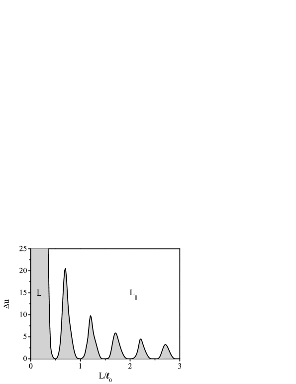
Figure 2: Phase diagram for intermediately segregated ($N\chi=20$) symmetric di-block lamellar phase in terms of the film thickness $L/\ell_{0}$ vs the surface field preference between the two blocks, $\Delta u=u_{A}-u_{B}$. The grey area indicates the perpendicular lamellar region (${\rm L}_{\perp}$) and the white region above it is the parallel state (${\rm L}_{||}$). The film is confined in the $z$-direction between two parallel and flat surfaces. The bottom surface uniformly attracts one of blocks ($\Delta u>0$), while the top one mimics the free (and neutral) surface, $\Delta u=0$.

In the remaining of the paper we will address in detail the question of how it is possible to better control the relative stability of parallel and perpendicular phases of lamellar BCP films. And, in particular, how can the stability of the perpendicular phase be increased for a larger range of film thicknesses and surface characteristics.

III Theoretical Framework

Since the system is translationally invariant in the $y$-direction, we treat it as an effective two-dimensional system. The free energy for such a di-block copolymer (BCP) film confined between the two surfaces is

$$\frac{a^{2}}{k_{B}T}{F} = \int{\rm d}^{2}r\left[\chi\phi_{A}(r)\phi_{B}(r)-\omega_{A}(r)\phi_{A}(r)-\omega_{B}(r)\phi_{B}(r)\right]$$ (1)

$$-{na^{2}}\ln Q_{C}-\int{\rm d}^{2}{r}\left[u_{A}(r)\phi_{A}(r)+u_{B}(r)\phi_{B}(r)\right]$$

$$+\int{\rm d}^{2}r\,\eta(r)[\phi_{A}(r)+\phi_{B}(r)-1]$$

where each of the $n$ BCP chains is composed of $N=N_{A}+N_{B}$ Kuhn segments of length $a$, and the Flory-Huggins parameter is $\chi$. The dimensionless volume fractions of the two components are defined as $\phi_{A}(r)=\phi_{A}(x,z)$ and $\phi_{B}(r)=\phi_{B}(x,z)$, respectively, whereas $\omega_{j}(r)$, $j={\rm A,B}$, are the auxiliary fields coupled with $\phi_{j}(r)$, and $Q_{C}$ is the single-chain partition function in the presence of the $\omega_{A}$ and $\omega_{B}$ fields [see Eqs. (4)-(5) below for more details]. The third term represents a surface energy preference, where $u_{A}$ and $u_{B}$ are the short-range interaction parameters of the surface with the A and B monomers, respectively. Formally, $u_{A}(r)$ and $u_{B}(r)$ are surface fields and get non-zero values only on the surface(s).

Finally, the last term includes a Lagrange multiplier $\eta(r)$ introduced to ensure the incompressibility condition of the BCP melt:

$$\phi_{A}(r)+\phi_{B}(r)=1\quad{\rm for~{}~{}all}\quad r\in\Omega$$ (2)

By inserting this condition, Eq. (2), in the surface free energy of Eq. (1), the integrand becomes $u_{A}\phi_{A}+u_{B}\phi_{B}=(u_{A}-u_{B})\phi_{A}+u_{B}$. Hence, $\Delta u(r)\equiv u_{A}(r)-u_{B}(r)$ is the only needed surface preference field that will be employed throughout the paper.

Using the saddle-point approximation, we obtain a set of self-consistent equations

$$\frac{\delta F}{\delta\phi_{A}}=0~{}\Rightarrow~{}~{}~{}\omega_{A}(r) = \chi\phi_{B}(r)-u_{A}(r)+\eta(r)$$

$$\frac{\delta F}{\delta\phi_{B}}=0~{}\Rightarrow~{}~{}~{}\omega_{B}(r) = \chi\phi_{A}(r)-u_{B}(r)+\eta(r)$$

$$\frac{\delta F}{\delta\omega_{A}}=0~{}\Rightarrow~{}~{}~{}\phi_{A}(r) = \frac{na^{2}}{\Omega Q_{C}}\int^{N_{A}}_{0}ds\,q_{A}(r,s)q^{{\dagger}}_{A}(r,N_{A}-s)$$

$$\frac{\delta F}{\delta\omega_{B}}=0~{}\Rightarrow~{}~{}~{}\phi_{B}(r) = \frac{na^{2}}{\Omega Q_{C}}\int^{N_{B}}_{0}ds\,q_{B}(r,s)q^{{\dagger}}_{B}(r,N_{B}-s)$$ (3)

where the incompressibility condition, Eq. (2), is obeyed, and the single-chain free energy $Q_{c}$ is:

$$Q_{C}=\frac{1}{\Omega}\int{\rm d}^{2}r\,q^{{\dagger}}_{A}(r,N_{A})$$ (4)

The two types of propagators $q_{j}\left(r,s\right)$ and $q^{{\dagger}}_{j}\left(r,s\right)$ (with $j={\rm A,B}$) are solutions of the modified diffusion equation

$$\frac{\partial q_{j}(r,s)}{\partial s}=\frac{a^{2}}{6}\nabla^{2}q_{j}\left(r,s\right)-\omega_{j}(r)q_{j}(r,s)$$ (5)

with the initial condition $q_{A}(r,s{=}0)\,{=}\,q_{B}(r,s{=}0)\,{=}\,1$, $q^{{\dagger}}_{A}(r,s{=}0)\,{=}\,q_{B}(r,N_{B})$ and $q^{{\dagger}}_{B}(r,s{=}0)\,{=}\,q_{A}(r,N_{A})$, where $s$ is a conveniently defined curvilinear coordinate along the chain contour. This diffusion equation is solved using reflecting boundary conditions at the two confining surfaces ($z=0$ and $z=L$): ${\rm d}q/{\rm d}r|_{z=0}\,{=}\,0$ and ${\rm d}q/{\rm d}r|_{z=L}\,{=}\,0$, while periodic boundary conditions are used in the perpendicular direction.

Hereafter, we rescale all lengths by the natural periodicity of the BCP, $\ell_{0}\simeq 4.05R_{g}$, ft2 where $R_{g}$ is the chain radius of gyration $R_{g}^{2}=Na^{2}/6$. Similarly, $s$ is rescaled by $N$, yielding $r\to r/\ell_{0}$, $s\to s/N$, $\chi\to N\chi$, $\omega_{j}(r)\to N\omega_{j}(r)$ and $u_{j}(r)\to Nu_{j}(r)$ with $j=$A or B. With this rescaling, we rewrite the self-consistent equations as:

$$\omega_{A}(r) = \chi\phi_{B}(r)-u_{A}(r)+\eta(r)$$ (6)

$$\omega_{B}(r) = \chi\phi_{A}(r)-u_{B}(r)+\eta(r)$$ (7)

$$\phi_{A}(r) = \frac{1}{Q_{C}}\int^{f}_{0}ds\,q_{A}(r,s)q^{{\dagger}}_{A}(r,f-s)$$ (8)

$$\phi_{B}(r) = \frac{1}{Q_{C}}\int^{1-f}_{0}ds\,q_{B}(r,s)q^{{\dagger}}_{B}(r,1-f-s)$$ (9)

$$\frac{\partial q_{j}(r,s)}{\partial s} = \left(\frac{R_{g}}{\ell_{0}}\right)^{2}\nabla^{2}q_{j}\left(r,s\right)-\omega_{j}(r)q_{j}(r,s)$$ (10)

where $f=N_{A}/N$, $\Omega_{1}\equiv\Omega/\ell^{2}_{0}$ and $Q_{C}=(1/{\Omega_{1}})\int{\rm d}^{2}r\,q^{{\dagger}}_{A}(r,f)$. Note that the incompressibility condition, Eq. (2), together with Eqs. (6) and (7) can be used to obtain the Lagrange multiplier $\eta(r)$

$$\eta(r)=\frac{1}{2}(\omega_{A}+\omega_{B}-\chi+u_{A}+u_{B})$$ (11)

With the rescaled variables, we define now a rescaled free energy:

$$\frac{Na^{2}}{\Omega_{1}\ell^{2}_{0}}\frac{F}{k_{B}T} = \frac{F}{nk_{B}T}=\frac{1}{\Omega_{1}}\int{\rm d}^{2}r\left[\chi\phi_{A}(r)\phi_{B}(r)-\omega_{A}(r)\phi_{A}(r)-\omega_{B}(r)\phi_{B}(r)\right]$$ (12)

$$- \ln Q_{C}-\frac{1}{\Omega_{1}}\int{\rm d}^{2}r\left[u_{A}(r)\phi_{A}(r)+u_{B}(r)\phi_{B}(r)\right]$$

$$+ \frac{1}{\Omega_{1}}\int{\rm d}^{2}r\,\eta(r)[\phi_{A}(r)+\phi_{B}(r)-1]$$

The above self-consistent equations can be solved numerically in the following way. First, we guess an initial set of values for the auxiliary fields $\omega_{j}(r)$. Then, through the diffusion equations, Eq. (10), we calculate the propagators, $q_{j}$ and $q^{\dagger}_{j}$. Next, we calculate the monomer volume fractions $\phi_{j}$ from Eqs. (8)-(9) and the Lagrange multiplier $\eta(r)$ from Eq. (10). We can now proceed with a new set of values for $\omega_{j}(r)$ obtained through Eqs. (6)-(7), and this procedure can be iterated until convergence is obtained by some conventional criterion described below.

We use the semi-implicit relaxation scheme fredrickson to solve the two-dimensional modified diffusion equations, Eq. (10). Our convergence criterion is based on the incompressibility condition. For perfect structures such as parallel or perpendicular lamellae, the maximum allowed deviation between the sum of the A and B densities and unity, $|1-\phi_{A}(r)-\phi_{B}(r)|$, is $10^{-4}$, whereas for the mixed L_M phase (see below), it is around $10^{-2}$. As mentioned above we rescale all lengths by the natural periodicity of the BCP, $\ell_{0}\simeq 4.05R_{g}$, and the curvilinear coordinate, $s$, by the total number of monomers in one chain, $N$. The spatial discretization in the $x$-direction is 0.05 (in units of $\ell_{0}$), while in the $z$-direction it is 0.025. The discretization of the $s$ variable is 0.02. For all the presented results, the free energy changes in the last few iteration steps are less than $10^{-4}$ in units of $k_{B}T/{\rm chain}$ after the first 1,000 iterations and decreases to $10^{-6}$ after additional 4,000 iterations. Note that since we work at a mean-field level (SCFT), it would not be of advantage to further refine the convergence of the free energies to a higher accuracy, since we neglect anyway quadratic fluctuations that might give larger corrections.

IV Results

We present now the numerical results for symmetric di-block films ($f=1/2$) at various patterned surfaces. The natural periodicity of the BCP, $\ell_{0}$, is chosen for all the numerical calculations to be $50$ nm. This value roughly corresponds to values used in several experimental set-ups r12 ; r15a ; r15b . All lengths are rescaled by $\ell_{0}$ as was explained in Sec. III. Except when explicitly mentioned, all results are obtained by using the fully disordered phase of the BCP film, $\phi_{A}(r)=\phi_{B}(r)=0.5$, as initial condition. Then, a temperature quench is performed from the disordered state above the ODT to temperatures below the ODT where the lamellar phase is stable.

IV.1 Chemically striped surface

The system is modeled using a SCFT scheme for two separate set-ups that are motivated by recent experiments r9 ; r11 ; r12 ; r15a ; r15b . In the first set-up, the BCP film is spread on a flat but chemically patterned solid surface, while the second bounding surface is the free film/air interface, which is either neutral or has a slight preference towards one of the two BCP components. In our calculations we take this top surface to be always neutral. A top view of the bottom patterned surface can be seen in Fig. 3, and is composed of infinitely long stripes in the $y$-direction of width $\omega_{s}\sim 100$ nm that prefer the A component ($\delta u>0$). These stripes are separated by neutral inter-stripe regions of width $\omega_{n}$ having the same affinity for A and B ($\Delta u=0$). As the stripes are infinitely long in the $y$-direction, the chemical surface pattern has a one-dimensional square-wave shape and is periodic in the $x$-direction, $\Delta u(x+d)=\Delta u(x)$, with periodicity $d=\omega_{s}+\omega_{n}$

$$\Delta u(x) = u_{s}~{}~{}~{}{\rm for}~{}~{}~{}0<x\leq\omega_{s}$$

$$\Delta u(x) = u_{n}~{}~{}~{}{\rm for}~{}~{}~{}\omega_{s}<x\leq d$$ (13)

Note that we can write formally the surface preference field $\Delta u=u_{A}-u_{B}$ as $\Delta u(r)=\Delta u(x)\delta(z)$, where $\delta(z)$ is the Dirac delta function. All numerical values of $\Delta u$ are given hereafter in terms of its rescaled units, $\Delta u\to N\Delta u$.

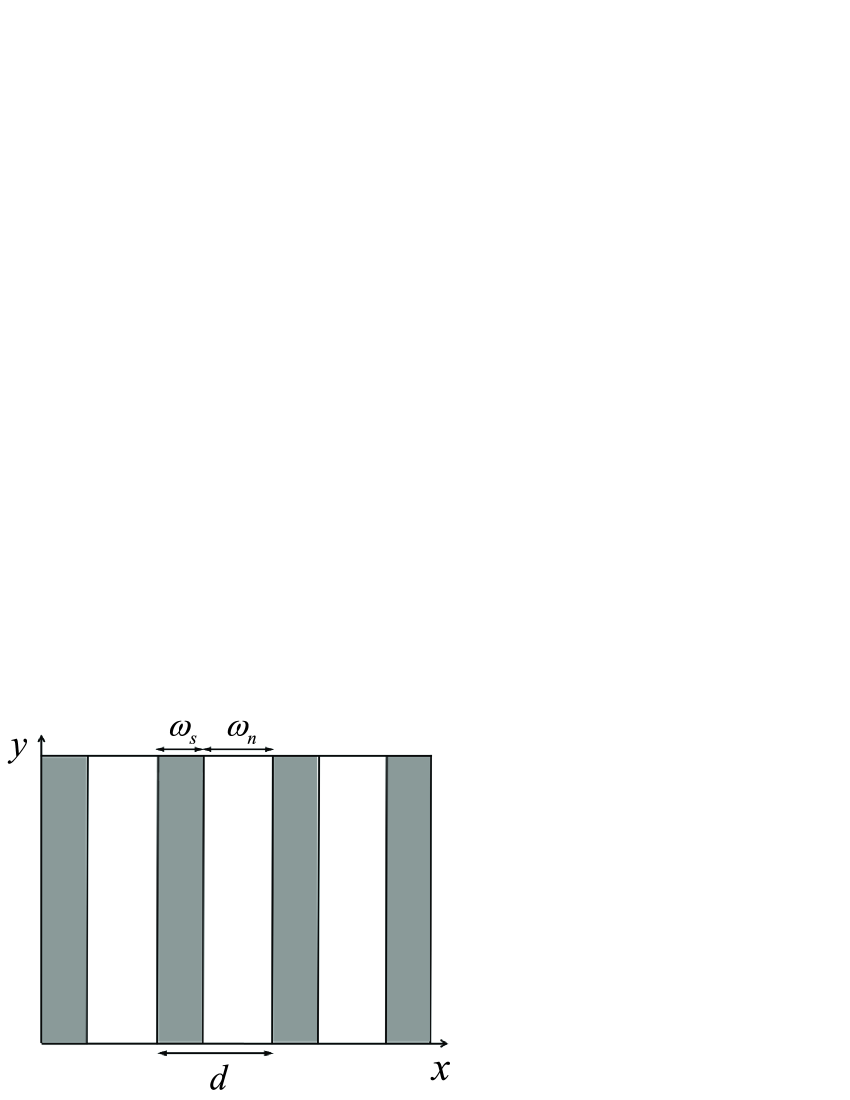
Figure 3: Top view of a striped surface lying in the $x-y$ plane. The periodicity is $d=\omega_{s}+\omega_{n}$, where the A-preferring stripes have a width of $\omega_{s}$ and the neutral inter-stripe regions are of width $\omega_{n}$.

Figure 4: Phase diagram in terms of the film thickness $L$ vs the surface preference $\Delta u$ for chemically striped surface (dashed line) and homogeneous surface (solid line). The lines separate the parallel phase (L_||) for larger $\Delta u$ values from perpendicular one (L_⟂) at smaller $\Delta u$ values, although the effective $\Delta u$ on the striped surface is $\Delta u_{\rm eff}=\Delta u(\omega_{s}/d$). The parameters used are $N\chi=20$, $\ell_{0}=50$ nm and for the striped surface: $\omega_{s}=2\ell_{0}$, $\omega_{n}=8\ell_{0}$ so that $d=10\ell_{0}=500$ nm.

In the following we fix the width $\omega_{s}$ to be twice the natural periodicity, yielding $\omega_{s}{=}2\ell_{0}{=}100$ nm. The phase diagram shown in Fig. 4 is calculated in terms of the film thickness, $L$, and the bottom surface preference, $\Delta u$, for this set-up and compared with the one in Fig. 2 for homogeneous surfaces. All parameters here are taken to be the same as for the homogeneous surface, except that the bottom surface has chemical stripes. Furthermore, we fix the value of the inter-stripe distance (where there is no preferred adsorption), to $\omega_{n}=8\ell_{0}=400$ nm so that the pattern periodicity is $d=\omega_{s}+\omega_{n}=500$ nm, or $10\ell_{0}$. The phase diagram is obtained by starting as an initial guess from the perpendicular lamellar phase (${\rm L}_{\perp}$) or the parallel one (${\rm L}_{||}$). After convergence, their free energies is compared. From the figure it is evident that the ${\rm L}_{\perp}$ phase has a larger stability range for the chemically striped surface as compared with the homogeneous surface, although the effective value of $\Delta u$ on the entire patterned surface is smaller as its value should be averaged over both the striped and inter-stripe regions: $\Delta u_{\rm eff}=\Delta u(\omega_{s}/d)$. Note that the stability of the L_⟂ phase is in particular enhanced for special values of $L$: $\frac{3}{4}\ell_{0},\frac{5}{4}\ell_{0}\dots$.

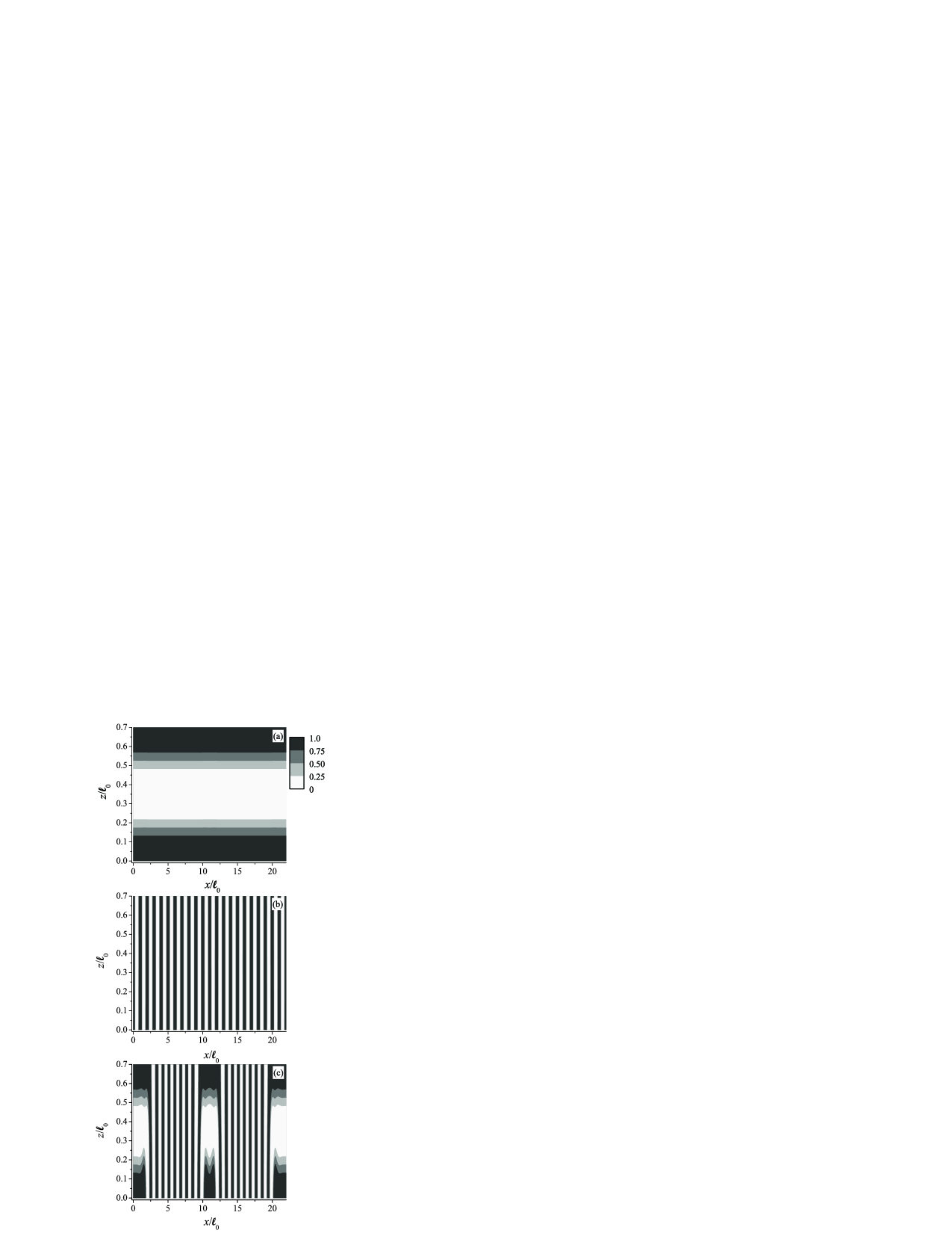
Figure 5: BCP lamellar structures obtained from numerical solutions of SCFT equations for three different initial conditions: (a) parallel lamellar (${\rm L}_{||}$); (b) perpendicular lamellar (${\rm L}_{\perp}$); and, (c) fully disordered state developing into a mixed morphology (${\rm L_{M}}$). The film thickness is $L=0.7\ell_{0}$, the top surface is taken as neutral, $\Delta u=0$, while the bottom one has a striped pattern as in Fig. 3 with $\Delta u=1$. The inter-stripe widths are set to be $\omega_{s}=2\ell_{0}$ and $\omega_{n}=8\ell_{0}$, yielding $d=\omega_{s}+\omega_{n}=10\ell_{0}=500$ nm. The other parameters are $N\chi=20$ and $\ell_{0}=50$ nm. The color code corresponds to the four intervals of local monomer density $0\leq\phi_{A}(r)\leq 1$, as is depicted in part (a).

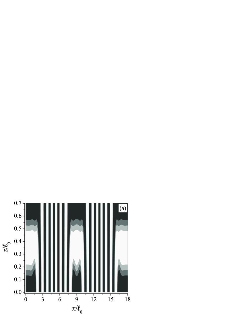
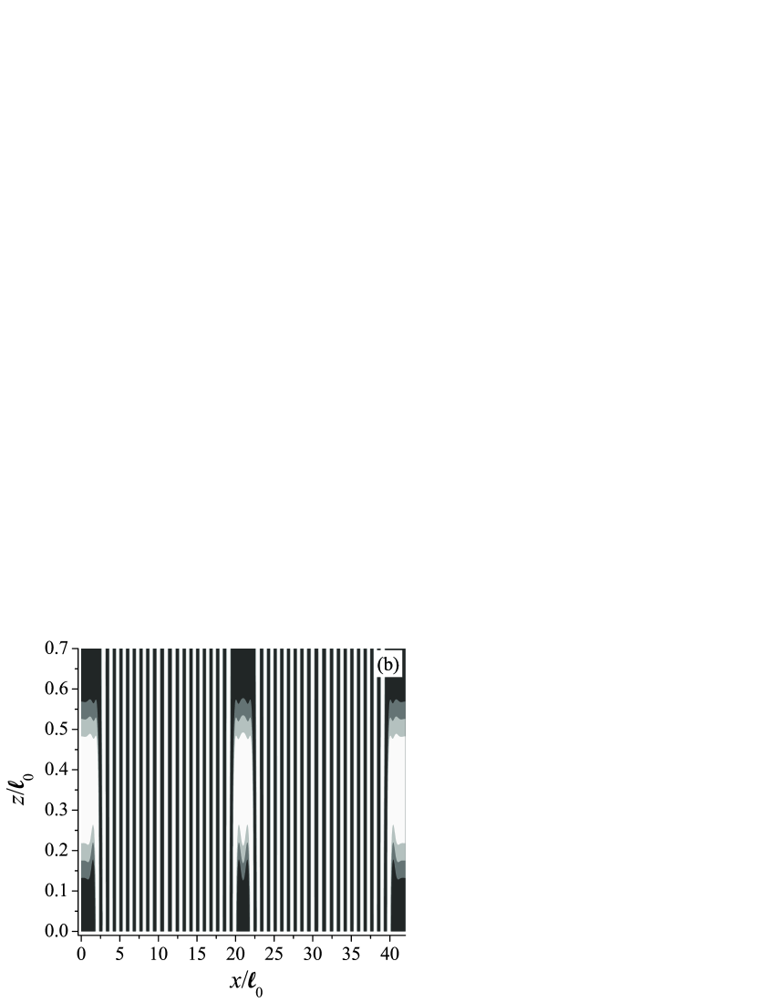
Figure 6: Calculated BCP lamellar structures for patterned surfaces of increasing inter-stripe distance while $\omega_{s}=2\ell_{0}$ remains fixed (and, hence, increasing $d$). In (a) $\omega_{n}=6\ell_{0}$ and $d=8\ell_{0}=400$ nm; in (b) $\omega_{n}=18\ell_{0}$ and $d=20\ell_{0}=1$ $\mu$m. All lengths are scaled with the lamellar periodicity $\ell_{0}=50$ nm. The other parameters are: $L=0.7\ell_{0}$, $\Delta u=1$, and $N\chi=20$. The initial condition is chosen as the fully disordered state, $\phi_{A}(r)=0.5$ and all other parameters and color code are the same as in Fig. 5. The system exhibits mixed ${\rm L_{M}}$ morphologies with L_|| regions just on top of the surface stripes and perfect L_⟂ domains in between the stripes.

Due to the existence of many metastable states in BCP melts, the numerical procedure of free energy minimization is sensitive to the initial conditions. Instead of converging always to the true equilibrium structure at any point of the phase diagram, different metastable structures can be obtained. We show some results to illustrate this scenario in Fig. 5.

For $L=0.7\ell_{0}$, $d=10\ell_{0}$, $\Delta u=1$ and $N\chi=20$ (a typical set of parameters that is located inside the ${\rm L}_{\perp}$ stable region), we start with parallel lamellae, perpendicular lamellae and the fully disordered state as three different initial conditions and perform a temperature quench to a temperature below the ODT. The ${\rm L}_{||}$ and ${\rm L}_{\perp}$ phases in Fig. 5a and 5b, respectively, result from quenching from ${\rm L}_{||}$ and ${\rm L}_{\perp}$ initial conditions. Hence, the system retains its orientation after the temperature quench. On the other hand, for the fully disordered initial condition, we obtain a mixed structure containing domains of the ${\rm L}_{||}$ and ${\rm L}_{\perp}$ phases. This structure is shown in Fig. 5c and is coined as ${\rm L_{M}}$.

As explained in Sec. III, the maximal deviation of the incompressibility condition, $|1-\phi_{A}(i,j)-\phi_{B}(i,j)|$, serves as our accuracy criterion. It is $1.10\times 10^{-6}$ for the parallel lamellae as initial condition (Fig. 5a); $2.57\times 10^{-5}$ for the perpendicular lamellae as initial condition (Fig. 5b); and, $1.07\times 10^{-2}$ for disordered state as initial condition (Fig. 5c). For the L_|| and L_⟂ it is quite small, yielding a value of about $10^{-5}$. However, it is not as good in the mixed L_M structure ($10^{-2}$), because of the existence of internal boundaries between parallel and perpendicular domains. To answer the question of metastability we calculate the free-energies per chain and obtain $f_{||}=4.272>f_{\rm M}=4.122>f_{\perp}=4.061$, corresponding to the ${\rm L}_{||}$, ${\rm L_{M}}$ and ${\rm L}_{\perp}$ phases, respectively. Clearly, the most stable structure is the perpendicular one, ${\rm L}_{\perp}$, and is consistent with our phase diagram in Fig. 4. Note that the free energy differences between the various states are very small, on the order of 2-5%, manifesting the tendency of the system to get trapped into metastable states.

Our findings have also experimental implications because in experiments the film structure depends strongly on its history and sample preparation r15b ; r29a ; r29b . The claim is that once the system is prepared in its ${\rm L}_{\perp}$ it will stay there. But if the film is prepared above the ODT, in its fully disordered state, the film can get stuck in a metastable mixed lamellar structure, ${\rm L_{M}}$. Although in experiments it is not always possible to heat the system above its ODT because of polymer break-down and oxidation, in many cases, higher temperatures are used to anneal the film and allow it to reach its final state via faster dynamics.

Another interesting feature is presented in Fig. 5. Perfect perpendicular lamellar structures between neighboring stripes are visible. Furthermore, we can obtain such perfect ${\rm L}_{\perp}$ structures for a wide range of small and large periodicities, ranging from $d=400$ nm in Fig. 6(a) to $d=1\,\mu{\mathrm{m}}=20\ell_{0}$ in Fig. 6(b). However, we find that it is difficult to get rid of the parallel lamellar regions induced by the striped pattern, even when we further reduce the BCP film thickness $L$ to values much less than $\ell_{0}$ and decrease the values of $\Delta u$. Furthermore, a preliminary study tobepublished indicates that slow temperature annealing from the disorder state (above ODT) to the ordered lamellar state (below ODT) does not seem to prevent the formation of the mixed ${\rm L_{M}}$ phase.

IV.2 Periodic grooved surfaces

In order to overcome the problem of getting trapped in ${\rm L_{M}}$ mixed states and inspired by recent NanoImprint lithography (NIL) experiments r15b ; r29 ; r29a ; r29b , we explored yet another type of surfaces. The set-up can be seen in Fig. 7, where the BCP film is confined between two solid surfaces. The bottom surface at $z=0$ is flat, while the top one has a periodic arrangement of grooves (along the $x$-direction) made of a series of down-pointing ‘fingers’ of thickness $\omega_{l}$, separated by inter-grooves regions (‘plateaus’) of thickness $\omega_{h}$. The periodic height profile $h(x)=h(x+d)$ has the form:

$$h(x) = L_{l}~{}~{}~{}{\rm for}~{}~{}~{}0<x\leq\omega_{l}$$

$$h(x) = L_{h}~{}~{}~{}{\rm for}~{}~{}~{}\omega_{l}<x\leq d$$ (14)

where the height is measured from the $z=0$ surface. Formally, $\Delta u(r)=u_{A}-u_{B}$ used in the solution of Eqs. (6)-(7) is given by $\Delta u(r)=\Delta u(x)\delta(z-h(x))$.

The figure shows the surface height profile in the $x-z$ plane, for profiles that are translationally invariant in the $y$-direction. The periodicity in the $x$-direction is $d=\omega_{l}+\omega_{h}$ and the finger width is chosen to be $\omega_{l}=5\ell_{0}=250$ nm. The top surface (mold) is put in direct contact with a BCP film spread on a neutral and flat bottom surface (at $z=0$). The distance of closest approach between the two surfaces is $L_{l}$, while the maximal height difference between them is $L_{h}$. This means that the finger height of the mold is $L_{h}-L_{l}$. Assuming film incompressibility, we get a relation between the thickness $L$ of the original BCP film and the two height parameters, $L_{l}$ and $L_{h}$: $L=(L_{l}\omega_{l}+L_{h}\omega_{h})/d$. In experiments, the average thickness $L$ is fixed, while in the numerical study, we control directly $L_{l}$ and $L_{h}$.

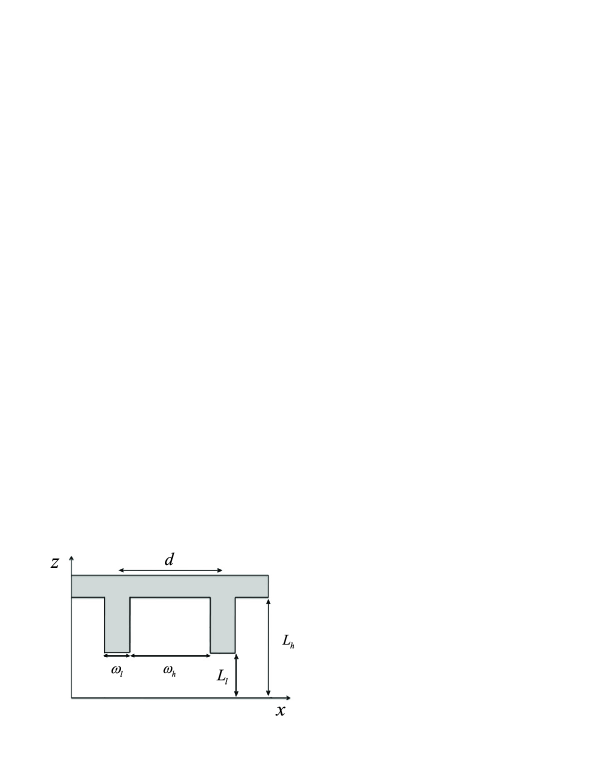
Figure 7: A cut (side view) through the top grooved surface (the mold). The periodicity in the $x$-direction is $d=\omega_{l}+\omega_{h}$, with $\omega_{l}$ and $\omega_{h}$ being the finger and inter-finger width, respectively. $L_{l}$ is the distance of closest approach to the bottom surface at $z=0$, and $L_{h}$ is the largest film thickness. The initial film thickness is equal to the average film thickness in the mold, $L=(L_{l}\omega_{l}+L_{h}\omega_{h})/d$.

By varying the values of the parameters $d$, $L_{h}$ and $L_{l}$ of the mold, and the strength of surface interactions $\Delta u$, we can get a sequence of BCP patterns. Furthermore, we obtain perfect perpendicular lamellar structures extending throughout the film thickness for some special patterned surfaces.

Figure 8: Phase diagram in terms of the maximal film thickness $L_{h}$ vs the surface field difference of the two blocks, $\Delta u$, for a periodic grooved surface (dashed line) and a homogeneous surface (solid line). In the latter case, the film thickness $L$ is equated with $L_{h}$. Other parameters are: $\ell_{0}=50$ nm, $L_{l}=0.3\ell_{0}$, $d=15\ell_{0}=750$ nm, $\omega_{l}=5\ell_{0}=250$ nm, $\omega_{h}=10\ell_{0}=500$ nm and $N\chi=20$.

We calculate the phase diagram in terms of the maximal film thickness, $L_{h}$, vs the surface preference, $\Delta u=u_{A}-u_{B}$. The interaction strength on all exposed surfaces of the upper grooved mold have the same value of $\Delta u$. In addition, we set $L_{l}=0.3\ell_{0}$, $d=10\ell_{0}$ and $\omega_{l}=5\ell_{0}$. The result is shown in Fig. 8, from which we can infer that this set-up greatly affects the phase diagram as compared with Fig. 2 for a uniform $\Delta u$ surface. The transition line from L_|| to L_⟂ is shifted upwards so that its minimum is obtained for $L_{h}=\ell_{0}$ where $\Delta u=4.4$. This is similar but more pronounced than the behavior seen in Fig. 4 for the chemical striped surface around the $L/\ell_{0}=1.0$ region.

However, when we start from a fully disordered state as initial condition inside the stable ${\rm L}_{\perp}$ region of Fig. 8 (e.g., $L_{h}=0.8\ell_{0}$ and $\Delta u=0.1$), we do not get the fully perpendicular lamellae ${\rm L}_{\perp}$ but rather a mixture of parallel and perpendicular lamellar regions (the ${\rm L_{M}}$ structure) as shown in Fig. 9.

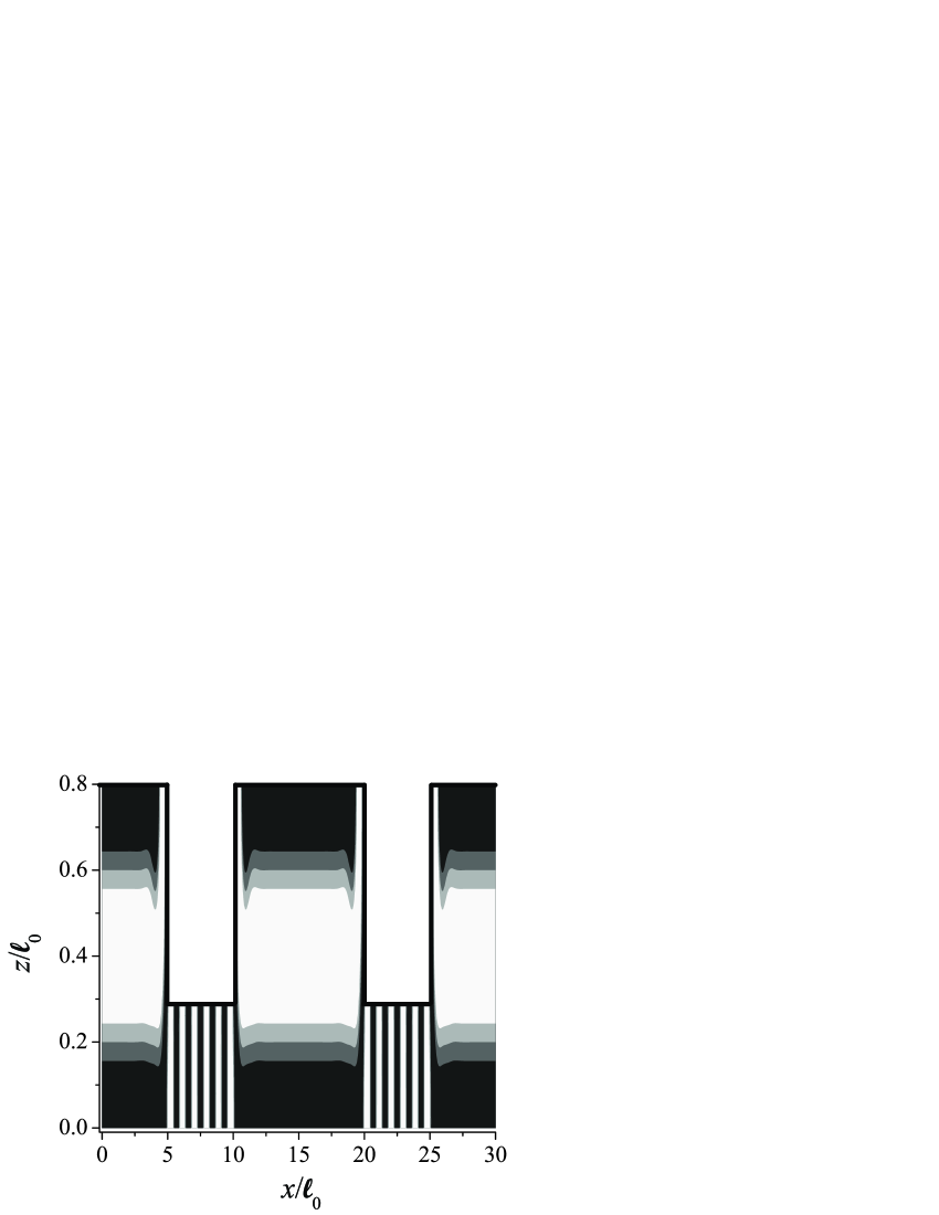
Figure 9: BCP density distribution for $d=15\ell_{0}=750$ nm and $N\chi=20$ starting from a fully disordered initial condition. The bottom surface is neutral and the top surface has a square wave height profile as in Fig. 8 where $\Delta u=0.1$. Other parameters are $L_{h}=0.8\ell_{0}$ and $L_{l}=0.3\ell_{0}$, $\omega_{h}=10\ell_{0}$, $\omega_{l}=5\ell_{0}$, yielding $L/\ell_{0}=1.9/3\simeq 0.64$.

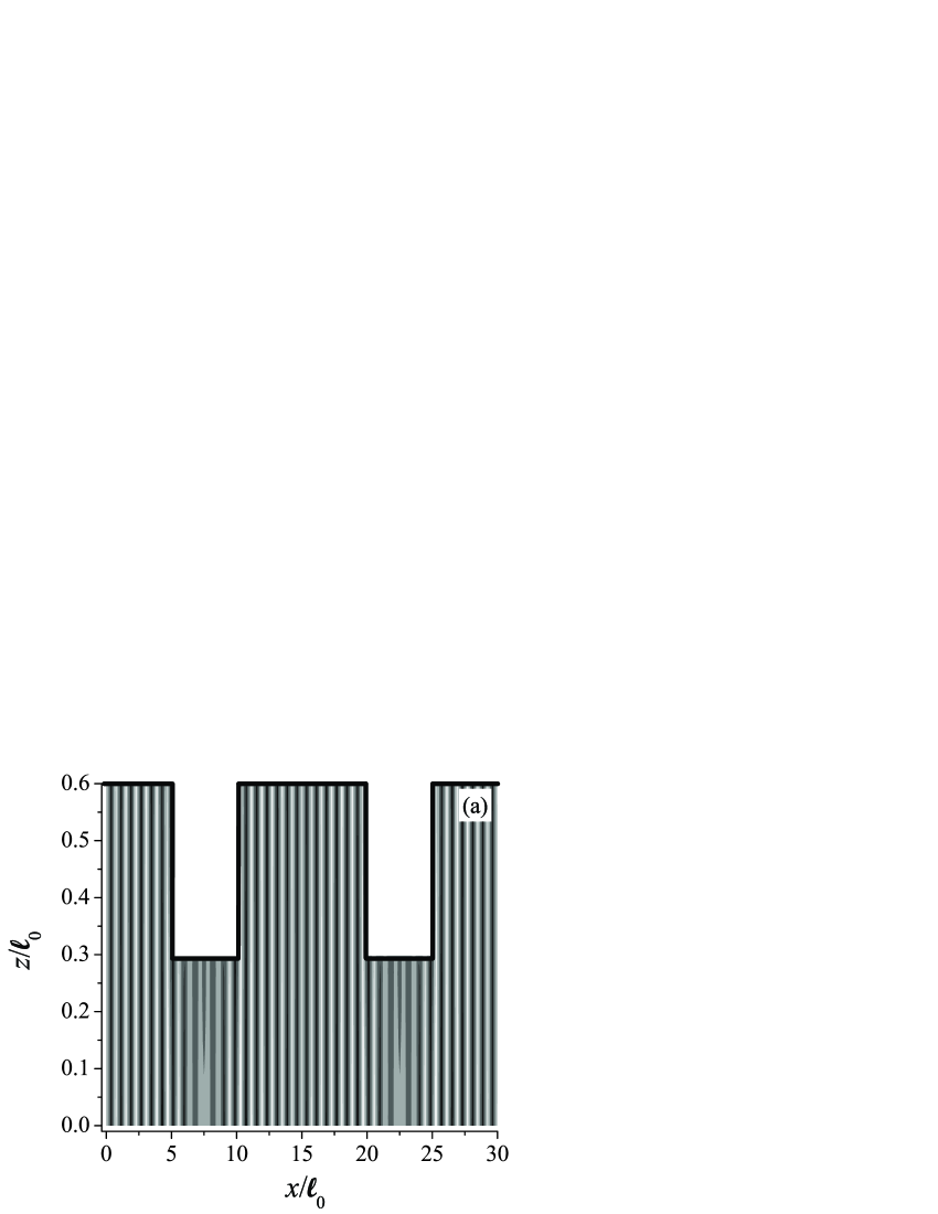
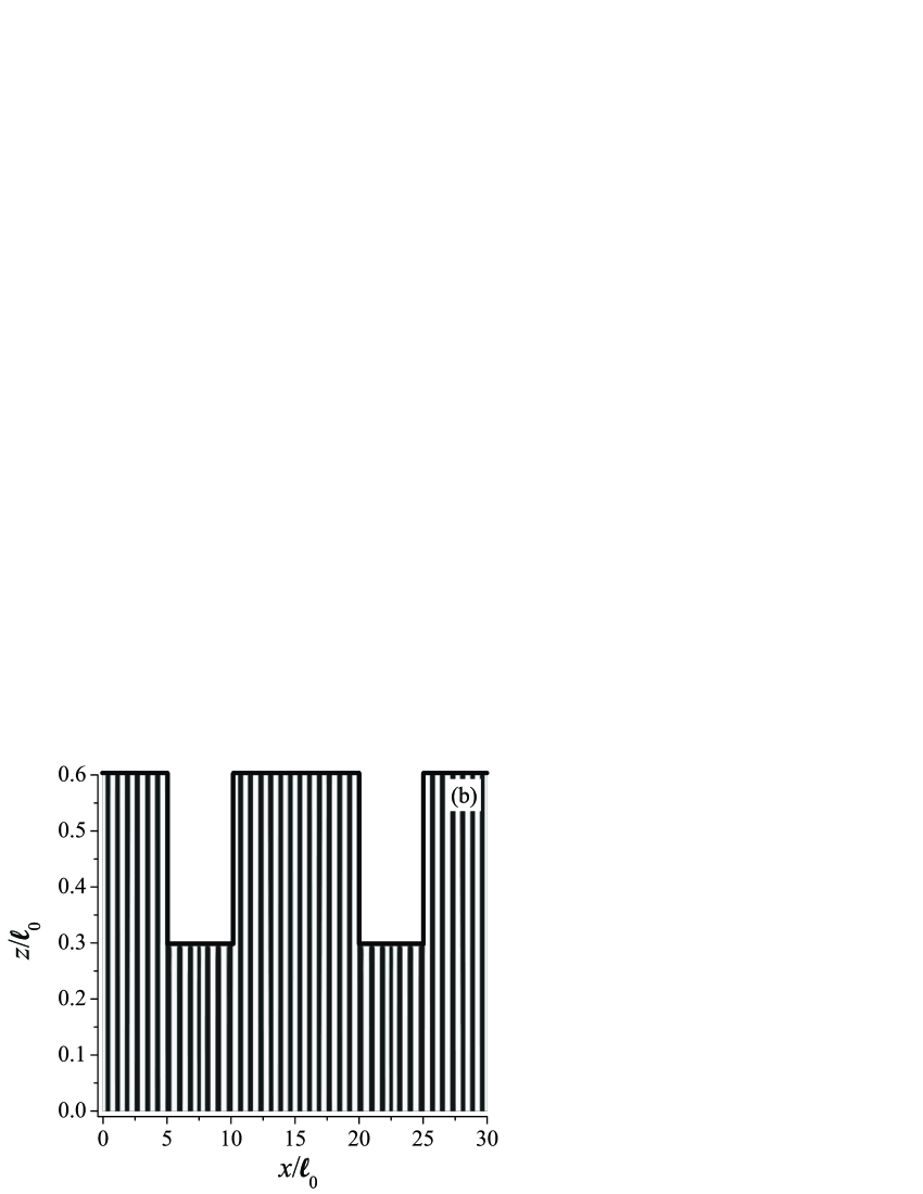
Figure 10: BCP density distribution for $d=15\ell_{0}=750$ nm and $N\chi=11.5$ when the initial condition is the fully disordered state. The system is first annealed to $N\chi=11.5$ in (a) and then to $N\chi=20$ in (b). The bottom surface ($z=0$) is neutral and the top surface has a square grooved structure with $\Delta u=0.1$. Other parameters are $L_{h}=0.6\ell_{0}$, $L_{l}=0.3\ell_{0}$, $\omega_{h}=10\ell_{0}$ and $\omega_{l}=5\ell_{0}$, yielding $L=0.5\ell_{0}$.

We find two ways to improve on the perpendicular orientation by changing the mold geometry and surface characteristics. First, we decrease the film thickness by decreasing $L_{h}$ to $0.6\ell_{0}$. In this case, we do a gradual temperature quench, starting from the disordered state above the ODT and quenching to temperatures just below the ODT, $N\chi=11.5$, and only then proceed with a deep quench to $N\chi=20$. This two-step procedure is shown in Fig. 10(a) and (b). Perfect perpendicular lamellar structures emerge. Moreover, using this two-step procedure we can even obtain a perfect perpendicular lamellar structures with much wider $\omega_{n}$ yielding $d=1.25$ $\mu$m (or equivalently $d/\ell_{0}=25$), as is shown in Fig. 11.

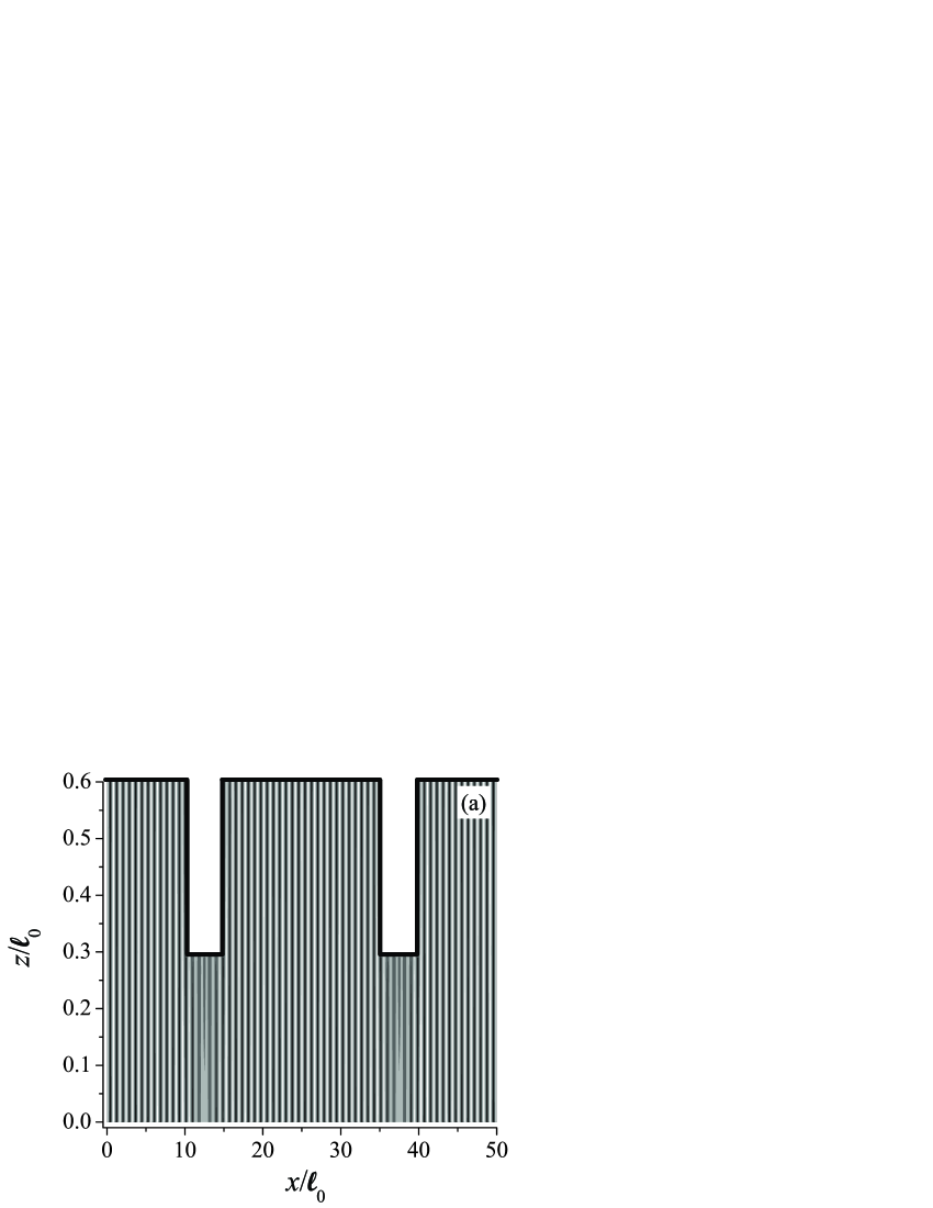
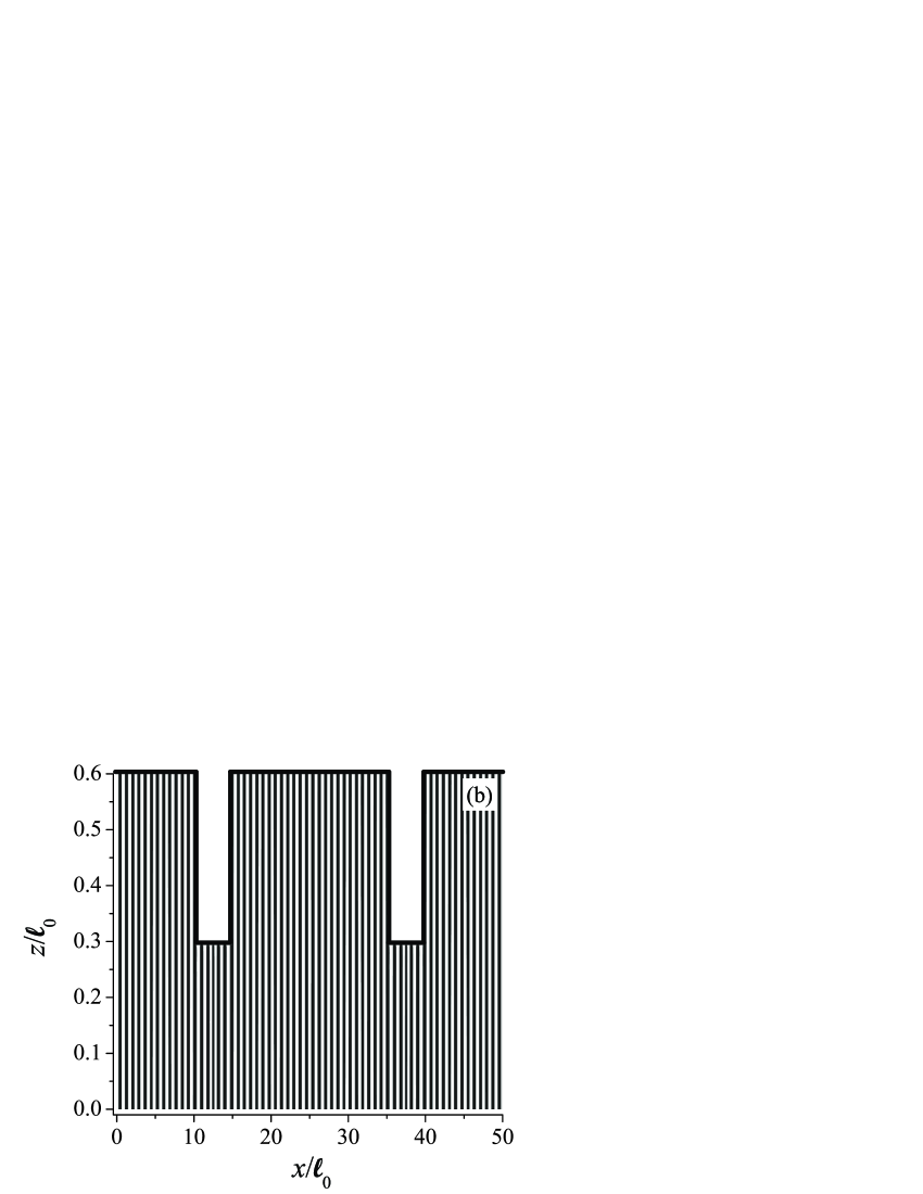
Figure 11: BCP density distribution for $d=25\ell_{0}=1.25$ $\mu$m using two-step annealing procedure. First to $N\chi=11.5$ in (a) and then to $N\chi=20$ in (b). The initial condition is the fully disordered state. Other parameters are: $L_{h}=0.6\ell_{0}$, $\omega_{l}=5\ell_{0}$, $\omega_{h}=20\ell_{0}$ and $L_{l}=0.3\ell_{0}$, yielding $L=0.54\ell_{0}$.

A second variation is to construct the grooves from two separate materials with different A/B preference. The protruding ‘finger’ parts are assumed to have a small A preference ($\Delta u=u_{1}>0$) both on their vertical and horizontal parts, while the high plateau parts are taken as neutral ($\Delta u=0$).

$$\Delta u(x) = u_{1}~{}~{}~{}{\rm for}~{}~{}~{}0\leq x\leq\omega_{s}$$

$$\Delta u(x) = 0~{}~{}~{}~{}{\rm for}~{}~{}~{}\omega_{s}<x<d$$ (15)

With this special surface geometry and interactions, we obtain perfect ${\rm L}_{\perp}$ structures for wide range of film thicknesses. An example for such a set-up with $d=25\ell_{0}$ periodicity is shown in Fig. 12.

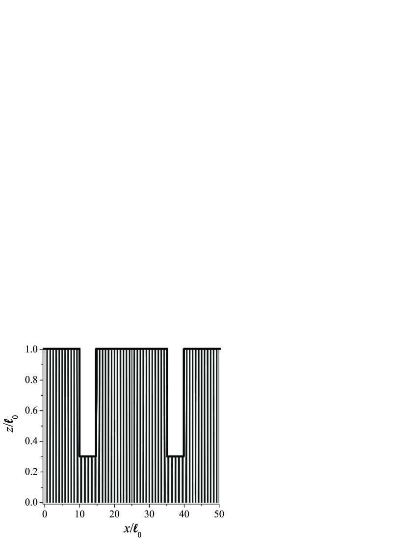
Figure 12: BCP density distribution for $d=25\ell_{0}=1.25$ $\mu$m. The bottom surface at $z=0$ is neutral, $\Delta u=0$. The top surface is a square grooved with $\Delta u=0.1$ on the sides and tips of the grooves and neutral ($\Delta u=0$) on the top plateau parts (see text) and Eq. (15). Other parameters are $N\chi=20$, $L_{h}=\ell_{0}$, $L_{l}=0.3\ell_{0}$, $\omega_{h}=20\ell_{0}$ and $\omega_{l}=5\ell_{0}$, yielding $L\simeq 0.86\ell_{0}$.

V Discussion and Conclusions

In this paper we addressed several surface patterns as inspired from recent experiments in relation with ordering and orientation of lamellar phases of block copolymer (BCP) films. In the first set-up, we model a BCP film confined between a chemical striped solid surface and the free film/air surface. In a second set-up, the film is considered to occupy the gap between two solid surfaces; a flat one and a hard mold with specific square-shape grooves as is inspired from recent NanoImprint lithography (NIL) experiments.

The main question both experiments and modeling should attempt answering is how to induce a perfect perpendicular order in BCP films? In particular, how this can be achieved using patterned surfaces with structural features (stripes and grooves) that have a periodicity $d$ much larger than the lamellar periodicity $\ell_{0}$. Having such sparse surface features will reduce substantially the cost of large-scale production of surface templates and BCP films and is essential for applications, e.g., in microelectronic and nano-lithography processes.

Using the first set-up of the chemically stripes on an otherwise flat and neutral surface, we are able to show that the perpendicular phase ${\rm L_{\perp}}$ has a larger stability region in parameter space described by the film thickness $L$ and surface preference ($\Delta u$), as compared with the homogeneous surface. Note that this is the case even for inter-stripe distances $\omega_{n}$ that are an order of magnitude larger than the stripe thickness, $\omega_{s}$. This is in spite the fact that the effective (averaged) $\Delta u$ for the striped surface is smaller than the corresponding $\Delta u$ on the homogeneous surface, $\Delta u_{\rm eff}=\Delta u(\omega_{s}/d)<\Delta u$. We equally find that the system is very sensitive to initial conditions. Starting from a fully disordered state, above the order-disorder temperature (ODT) and annealing the temperature into the lamellar region, will mainly produce a mixed morphology ${\rm L_{M}}$ as can be seen in Fig. 5(c) and Fig. 6. Although the stripes nucleate growth of BCP layers on top of them (namely, domains with parallel orientation, ${\rm L_{||}}$), perfectly oriented perpendicular domains, ${\rm L_{\perp}}$, are induced on top of the neutral inter-stripe region.

In our model the L_M mixed morphology is a result of the large number of metastable states (local minima) which the system possesses. Although the true equilibrium is the ${\rm L_{\perp}}$ phase, it is hard to find it numerically unless one starts with the proper initial conditions. This drawback should also be expected in experiments, where during sample preparation, the film undergoes many external stresses and defects are abundant. It will be of interest to verify in experiment our findings by doing a slow temperature annealing of BCP films from their disordered liquid state (above ODT) into the lamellar region (below the ODT). Such a slow temperature annealing has the potential to produce highly oriented BCP films. Although not in all systems it is possible to reach temperatures above the ODT without damaging the BCP chains, we equally note that in many cases annealing at high enough temperatures has the advantage that the system can reach it final state with faster kinetics.

In the second set-up, we modeled a hard mold which is pressed onto a BCP lamellar film. We show that this NanoImprint lithography (NIL) process greatly enhances perpendicular order in lamellar phases. Perfect ${\rm L_{\perp}}$ can be seen for film thicknesses below $\ell_{0}$ even when the groove width $\omega_{h}$ (filled with the BCP film) is five times (or even larger) than the solid ‘finger’ ($\omega_{l}$) sections. Here the slow annealing from above ODT to below the ODT is very successful, demonstrating that this set-up is more suitable for lamellar orientation purposes than the chemical stripe set-ups discussed above.

In Fig. 12 we proposed a mold with even superior orientation qualities. For this mold the surface preference of the downward protrusion sections (the ‘fingers’) is larger than that of the top section of the groove (plateau-like). As the latter preference interferes with the ${\rm L_{||}}$ ordering, reducing this surface preference will enhance ${\rm L_{\perp}}$ ordering, especially in the desired case of thin fingers and wide plateaus, where $\omega_{h}\gg\omega_{l}$.

In experiments, it is harder to produce a mold with such specific surface characteristics as seen in Fig. 12. One way would be to form it from two separate materials or to use a selective coating during mold preparation. However, creating such a mold can be a costly and delicate process that will be hard to mass reproduce. Yet another possibility is to have an effective chemically heterogeneous mold shown in Fig. 13. Suppose that the groove height is only partially filled with the BCP melt, creating pockets of air on the top of each groove r29 . The film/air interface within each groove can be thought of as another interface with almost neutral preference the two blocks. This situation amounts to taking different values of $\Delta u$ on the finger-section and plateau-section of the mold [see Eq. (15)]. While $\Delta u=0$ on the top section (plateau) of the groove, it is non-zero on the mold ‘finger’ sections. This is exactly the situation explored in our calculations and shown in Fig. 12, and it may be worthwhile to further explore this partial filled mold in future experiments.

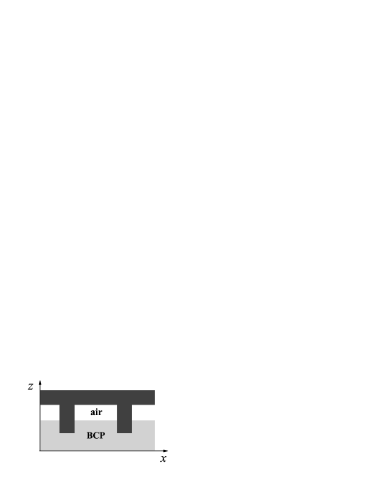
Figure 13: Schematic drawing of the NanoImprint lithography (NIL) set-up where the mold only partially is filled with the BCP film. Effectively, this means that the film sections in contact with the side boundaries of mold feel a different surface field than the top horizontal facets, which are exposed to the air.

Our theoretical modeling relies on numerical solutions of self-consistent field theory (SCFT) equations. We minimize the corresponding free energies and converge to film morphology whose free energy is an extremum using an iterative procedure. We find that the numerical procedure is sensitive to what is used as initial conditions for the BCP structure. The convergence can be towards local (metastable) states and not always towards the true equilibrium. This is an unavoidable feature of the numerical procedure. It is not an artifact but rather reflects the true physical situation as seen in experiment. The BCP film has many metastable states separated by energy barriers and it is hard to reach the true thermodynamical equilibrium state. Slow annealing from above the ODT or from high temperatures is one way to overcome this difficulty, at least in a partial way.

It will be of great interest to further proceed and extend our two-dimensional calculations to full three-dimensional ones. This will require much longer computation times but will allow us to distinguish between perfectly oriented perpendicular lamellae and those that stand up but which also wander around in the $x-y$ plane. For applications it is important to have perfectly oriented ${\rm L_{\perp}}$ phases in the $z$-direction, that are well aligned in the lateral (in-plane) directions.

Although our present study is not exhaustive, it shows many possibilities of explaining some of the experimental findings and even points towards interesting directions for future experiments.

References

- (1) Hamley, I.W. The Physics of Block Copolymers, Oxford Univerity, Oxford, U.K., 1999.
- (2) Park, M.; Harrison, C.; Chaikin, P. M.; Register, R. A.; Adamson, D. H. Science , 276, 1401.
- (3) Li, R. R.; Dapkus, P. D.; Thompson, M. E.; Jeong, W. G.; Harrison, C.; Chaikin, P. M.; Register, R. A.; Adamson, D. H. Appl. Phys. Lett. , 76, 1689.
- (4) Lopes, W. A.; Jaeger, H. M. Nature , 414, 735.
- (5) Cheng, J. Y.; Ross, C. A.; Thomas, E. L.; Smith, H. I.; Vancso, G. J. Appl. Phys. Lett. , 81, 3657.
- (6) Park, C.; Yoon, J.; Thomas, E. L. Polymer, , 44, 6725.
- (7) Li, M.; Ober, C. K. Mater. Today , 9, 30.
- (8) Stoykovich, M. P.; Kang, H.; Daoulas, K. C.; Liu, G. L.; Liu, C.-C.; de Pablo, J. J.; Müller, M.; Nealey, P. F. ACS Nano , 1, 168.
- (9) Mansky, P.; Liu, Y.; Huang, E.; Russell, T. P.; Hawker, C. J. Science , 275, 1458.
- (10) Yang, X. M.; Peters, R. D.; Nealey, P. F.; Solak, H. H.; Cerrina, F. Macromolecules , 33, 9575.
- (11) Kim, S. O.; Solak, H. H.; Stoykovich, M. P.; Ferrier, N. J.; de Pablo, J. J.; Nealey, P. F. Nature , 424, 411.
- (12) Stoykovich, M. P.; Müller, M.; Kim, S. O.; Solak, H. H.; Edwards, E. W.; de Pablo, J. J.; Nealey, P. F. Science , 308, 1442.
- (13) Liu, P.-H.; Thebault, P.; Guenoun, P.; Daillant, J. Macromolecules , 42, 9609.
- (14) Man, X. K.; Andelman, D.; Orland, H.; Thébault, P.; Liu, P.-H.; Guenoun, P.; Daillant, J., Landis, S. Soft Matter, 2010, to be published.
- (15) Segalman, R. A.; Yokoyama, H.; Kramer, E. J. Adv. Mater. , 13, 1152.
- (16) Ruiz, R.; Kang, H.; Detcheverry, F. A.; Dobisz, E.; Kercher, D. S.; Albrecht, T. R.; de Pablo, J. J.; Nealey, P. F. Science , 321, 936.
- (17) Bita, I.; Yang, J. K. W.; Jung, Y. S.; Ross, C. A.; Thomas, E. L.; Berggren, K. K. Science , 321, 939.
- (18) Sundrani, D.; Darling, S. B.; Sibener, S. J. Nano. Lett. , 4, 273.
- (19) Cheng, J. Y.; Mayes, A. M.; Ross, C. A. Nat. Mater. , 3, 823.
- (20) Ryu, D. Y.; Wang, J.-Y.; Lavery, K. A.; Drockenmuller, E.; Satija, S. K.; Hawker, C. J.; Russell, T. P. Macromolecules , 40, 4296.
- (21) Ham, S. J.; Shin, C.; Kim, E.; Ryu, D. Y.; Jeong, U.; Russell, T. P.; Hawker, C. J. Macromolecules , 41, 6431.
- (22) Park, S.; Lee, D. H.; Xu, J.; Kim, B.; Hong, S. W.; Jeong, U.; Xu, T.; Russell, T. P. Science , 323, 1030.
- (23) Pereira, G. G.; Williams, D. R. M. Macromolecules , 32, 8115.
- (24) Böker, A.; Knoll, A.; Elbs, H.; Abetz, V.; Müller, A. H. E.; Krausch, G. Macromolecules , 35, 1319.
- (25) Tsori, Y.; Andelman, D. Macromolecules , 35, 5161.
- (26) Tsori, Y.; Tournilhac, F.; Andelman, D.; Leibler. L. W. Phys. Rev. Lett. , 90, 145504.
- (27) Lin, C.-Y.; Schick, M.; Andelman, D. Macromolecules , 38, 5766.
- (28) Tsori, Y.; Andelman, D.; Lin, C.-Y.; Schick, M. Macromolecules , 39, 289.
- (29) Lin, C.-Y.; Schick, M. J. Chem. Phys. , 125, 034902.
- (30) Matsen, M. W. Macromolecules , 39, 5512.
- (31) Matsen, M. W. Soft Matter , 2, 1048.
- (32) Li, H. W.; Huck, W. T. S. Nano Lett. , 4, 1633.
- (33) Kim, S.; Lee, J.; Jeon, S.-M.; Lee, H.H.; Char, K.; Sohn, B.-H. Macromolecules , 41, 3401.
- (34) Thébault, P.; Niedermayer, S.; Landis, S.; Guenoun, P.; Daillant, J. Man, X. K.; Andelman, D.; Orland, H. Adv. Mater. , 24, 1952.
- (35) For off-symmetrical fraction, , the equilibrium state is either asymmetric lamellae or phases of completely different symmetry such as hexagonal phases of cylinders or others (see Ref. HamleyBook ). These latter phases will not be considered in this paper.
- (36) Tsori, Y.; Andelman, D. Eur. Phys. J. E. , 5, 605.
- (37) Semenov, A. N. Sov. Phys. JETP , 61, 733.
- (38) Matsen, M. W. J. Chem. Phys. , 106, 7781.
- (39) Petera, D.; Muthukumar, M. J. Chem. Phys. , 109, 5101.
- (40) Kielhom, L.; Muthukumar, M. J. Chem. Phys. , 111, 2259.
- (41) Pereira, G. G.; Williams, D. R. M. Europhys. Lett. , 44, 302.
- (42) Pereira, G. G.; Williams, D. R. M. Macromolecules , 32, 758.
- (43) Geisinger, T.; Mueller, M.; Binder, K. J. Chem. Phys. , 111, 5241.
- (44) Tsori, Y.; Andelman, D. J. Chem. Phys. , 115, 1970.
- (45) Tsori, Y.; Andelman, D. Europhys. Lett. , 53, 722.
- (46) Tsori, Y.; Andelman, D. J. Polymer Science: Part B: Polymer Physics , 44, 2725.
- (47) The natural period of BCP, , is proportional to the chain radius of gyration, . In our numerical SCFT scheme the factor of proportionality is found to be 4.05, i.e., . This is very close to the value obtained in Ref. r30 , .
- (48) Ceniceros, H. D.; Fredrickson, G. H. Mult. Mod. Simulat. 2004, 2, 452.
- (49) Man, X. K. ; Andelman, D.; Orland, H. Macromolecules 2011, 44, 2206.