Conformal Hamiltonian Dynamics of General Relativity

Abstract

The General Relativity formulated with the aid of the spin connection coefficients is considered in the finite space geometry of similarity with the Dirac scalar dilaton. We show that the redshift evolution of the General Relativity describes the vacuum creation of the matter in the empty Universe at the electroweak epoch and the dilaton vacuum energy plays a role of the dark energy.

Submitted to Phys. Lett. B 14 April 2010; accepted 23 June 2002.

The distance-redshift dependence in the data of the type Ia supernovae [1] is a topical problem in the standard cosmology (SC). As it is known, the SNeIa distances are greater than the ones predicted by the SC based on the matter dominance idea [2]. There are numerous attempts to resolve this problem with a various degree of success (see for review [3]). One of the popular approaches is the $\Lambda$-Cold-Dark-Matter model [4]. It provides, however, the present-day slow inflation density that is less by factor of $10^{-57}$ than the fast primordial inflation density proposed to include the Planck epoch.

Approaches to the General Relativity (GR) with conformal symmetry provide a natural relation to the SC [5]. The Dirac version [6] of the geometry of similarity [7] is an efficient way to include the conformal symmetry into the GR. In fact, the latter approach allows to explain the SNeIa data without the inflation [8]. In the present paper, the Dirac formulation of the GR in the geometry of similarity is adapted to the diffeo-invariant Hamiltonian approach by means of the spin connection coefficients in a finite space-time, developed in [9]. In this way we study a possibility to choose variables and their initial data that are compatible with the observational data associated with the dark energy content. We find integrals of motion of the metric and matter fields in terms of the variables distinguished by the conformal initial data.

Within the Dirac approach the Einstein-Hilbert action takes the form

$$W_{\rm Hilbert}=-\int\limits d^{4}x|-e|\frac{1}{6}R(e)\bigg{|}_{e=e^{-D}\widetilde{e}}$$

$$=-\int\limits d^{4}x\biggl{[}\frac{|-\widetilde{e}|e^{-2D}}{6}R(\widetilde{e})-e^{-D}\partial_{\mu}\left(|-\widetilde{e}|\widetilde{g}^{\mu\nu}\partial_{\nu}e^{-D}\right)\biggr{]}.$$ (1)

Hereafter, we use the units $M^{2}_{\rm Planck}\frac{3}{8\pi}=1$. The interval is defined via diffeo-invariant linear forms $\omega_{(\alpha)}=e_{(\lambda)\mu}dx^{\mu}$ with the tetrad coefficients

$$ds^{2}\!=\!g_{\mu\nu}dx^{\mu}dx^{\nu}=\omega_{({\alpha})}(d)\otimes\omega_{({\beta})}(d)\eta_{({\alpha})({\beta})};~{}~{}\eta_{({\alpha})({\beta})}\!=\!Diag(1,\!-1,\!-1,\!-1).$$ (2)

The geometry of similarity [6, 7] means the identification of measured physical quantities ${F}^{(n)}$, where $(n)$ is the conformal weight, with their ratios in dilaton units $e^{-nD}$

$$\widetilde{F}^{(n)}=e^{nD}{F}^{(n)},\qquad\widetilde{ds}^{2}=e^{2D}ds^{2}.$$ (3)

We define the measurable space-time coordinates in the GR as the scale-invariant quantities in the framework of the Dirac-ADM 4=1+3 foliation [10, 11]

$$\widetilde{ds}^{2}={\widetilde{\omega}}_{(0)}\otimes{\widetilde{\omega}}_{(0)}-{\widetilde{\omega}}_{(b)}\otimes{\widetilde{\omega}}_{(b)},$$ (4)

where the linear forms ${\widetilde{\omega}}_{(\alpha)}=\widetilde{e}_{(\alpha)\mu}dx^{\mu}$ are

$${\widetilde{\omega}}_{(0)}=e^{-2{D}}Ndx^{0},$$ (5)

$${\widetilde{\omega}}_{(b)}=\overline{\omega}_{(b)}+{\bf e}_{(b)j}N^{j}dx^{0},$$ (6)

$${\overline{\omega}}_{(b)}={\bf e}_{(b)i}dx^{i}.$$ (7)

Here ${N}$ is the Dirac lapse function, $N^{j}$ are the shift vector components, and ${\bf e}_{(b)i}$ are the triads corresponding to the unit spatial metric determinant $|\widetilde{g}^{(3)}_{ij}|\equiv|{\bf e}_{(b)j}{\bf e}_{(b)i}|=1$.

The Dirac dilaton $D=-(1/6)\log|{g}^{(3)}_{ij}|=\langle D\rangle+{\overline{D}}$, is taken in the Lichnerowicz gauge [12]. The Dirac lapse function ${N}=N_{0}(x^{0}){\cal N}(\tau,x)$ is split on the global factor $N_{0}^{-1}=\langle N^{-1}\rangle$ which determines all time intervals used in the observational cosmology: the redshift interval $d\tau=N_{0}dx^{0}$ [13], the conformal one $d\eta=d\tau e^{-2\langle D\rangle}$, and the world interval $dt=e^{-\langle D\rangle}d\eta=d\tau e^{-3\langle D\rangle}$. In this case the dilaton zeroth mode $\langle D\rangle=V_{0}^{-1}\int_{V_{0}}d^{3}xD$ (defined in the finite diffeo-invariant volume) coincides with the logarithm of the redshift of spectral line energy $E_{\rm m}$

$$\langle D\rangle=\log(1+z)=\log\left(E_{\rm m}(\eta_{0}-\eta)/E_{\rm m}(\eta_{0})\right),$$ (8)

where $\eta_{0}$ is the present-day conformal time interval, and $\eta_{0}-\eta=r/c$ is the SNeIa distance. In accord with the new Poincaré group classification, the ”redshift” (8) is treated as one of the matter components, on the equal footing with the matter.

The key point of our approach is to express the GR action directly in terms of the redshift factor. The action can be represented as a sum of the dilaton and the graviton terms:

$${W}_{\rm Hilbert}=\int\limits dx^{0}\left[-\dfrac{\left(\partial_{0}\langle D\rangle\right)^{2}}{N_{0}}+N_{0}e^{-2\langle D\rangle}\textsf{L}_{g}\right],$$ (9)

$$\textsf{L}_{g}=e^{2\langle D\rangle}\int d^{3}x{\cal N}\left[-(v_{\overline{D}})^{2}+\dfrac{v^{2}_{(ab)}}{6}-e^{-4D}\dfrac{R^{(3)}}{6}\right].$$ (10)

Here,

$$R^{(3)} = R^{(3)}({\bf e})-\frac{4}{3}{e^{7D/2}}\triangle e^{-D/2},$$ (11)

is the curvature, where $R^{(3)}({\bf e})$ is expressed via the spin-connection coefficients

$$\omega^{\pm}_{(ab)}(\partial_{(c)}) = \frac{1}{2}\left[{\bf e}^{j}_{(a)}\partial_{(c)}{\bf e}^{j}_{(b)}\pm{\bf e}^{i}_{(b)}\partial_{(c)}{\bf e}^{i}_{(a)}\right]\,\,,$$ (12)

and $\triangle=\partial_{i}[{\bf e}^{i}_{(a)}{\bf e}^{j}_{(a)}\partial_{j}]$ is the Laplace operator.

The dependence of the linear forms

$${\overline{\omega}}_{(b)}(d)={\bf e}_{(b)i}dx^{i}=dX_{(b)}-X_{(c)}{\bf e}^{i}_{(c)}d{\bf e}_{(b)i}$$ (13)

on the tangent space coordinates $X_{(b)}\equiv\int dx^{i}{\bf e}_{(b)i}=x^{i}{\bf e}_{(b)i}$ by means of the spin connection coefficients can be obtained by virtue of the Leibniz rule $AdB=d(AB)-(AB)d\log(A)$ (in particular $d[x^{i}]{\bf e}^{T}_{\underline{b}i}=d[x^{i}{\bf e}^{T}_{\underline{b}i}]-x^{i}d[{\bf e}^{T}_{\underline{b}i}]$). The difference between this approach to gravitation waves and the accepted one [14, 15] is that the symmetry with respect to diffeomorphisms is imposed on spin connection coefficients.

The linear graviton form (12) can be expressed via two photon-like polarization vectors $\varepsilon^{(\alpha)}_{(a)}(\textbf{k})$. By virtue of the condition

$${\sum_{\alpha=1,2}\varepsilon^{(\alpha)}_{(a)}(\textbf{k})\varepsilon^{(\alpha)}_{(b)}(\textbf{k})=\delta_{(a)(b)}-\dfrac{\textbf{k}_{(a)}\textbf{k}_{(b)}}{\textbf{k}^{(2)}}},$$ (14)

one obtains

$$\omega^{+}_{(ab)}(\partial_{(c)})=\sum_{\textbf{k}^{2}\not=0}\dfrac{e^{i\textbf{{k}{X}}}}{\sqrt{2\omega_{\textbf{k}}}}\textbf{k}_{(c)}[\varepsilon^{R}_{(ab)}(\textbf{k})g_{\textbf{k}}^{+}(\eta)+\varepsilon^{R}_{(ab)}(-\textbf{k})g_{\textbf{k}}^{-}(\eta)],$$ (15)

where ${\varepsilon}^{R}_{(ab)}(\textbf{k})={\rm diag}[1,-1,0]$ in the orthogonal basis of spatial vectors $[\vec{\varepsilon}\,^{(1)}(\textbf{k})$, $\vec{\varepsilon}\,^{(2)}(\textbf{k})$, ${\textbf{k}}]$. Here, $g^{\pm}$ are the holomorphic variables of the single degree of freedom, $\omega_{\textbf{k}}=\sqrt{{\textbf{k}}^{2}}$ is the graviton energy normalized (like a photon in QED) on the units of a volume and time

$$\overline{g}_{\textbf{k}}^{\pm}=\dfrac{\sqrt{8\pi}}{M_{\rm Planck}V^{1/2}_{0}}g_{\textbf{k}}^{\pm}.$$ (16)

The triad velocities

$$v_{(ab)}=\frac{1}{N}\left[\omega^{+}_{(a)(b)}(\partial_{0}-N^{l}\partial_{l})+\partial_{(a)}N^{\bot}_{(b)}+\partial_{(a)}N^{\bot}_{(b)}\right]$$ (17)

depend on the symmetric forms $\omega^{+}_{(ab)}$, and the shift vector components $\partial_{(b)}N^{\bot}_{(b)}=0$ are treated as the non-dynamical potentials. This means that the anti-symmetric forms $\omega^{-}_{(ab)}$ are not dynamically independent variables but are determined by a matter distribution.

Following Dirac [10, 16] one can define such a coordinate system, where the covariant velocity $v_{{\overline{D}}}$ of the local volume element and the momentum

$$P_{{\overline{D}}}=2v_{\overline{D}}=\frac{2}{N}\left[(\partial_{0}-N^{l}\partial_{l}){\overline{D}}+\partial_{l}N^{l}/3\right]=0$$ (18)

are zero. As a result, the dilaton deviation $\overline{D}$ can be treated as a static potential. The dilaton contribution to the curvature (11) with matter sources yield the Schwarzschild solution of classical equations $\triangle[\exp\{-7\overline{D}/2\}{\cal N}]=0$ and $\triangle\exp\{-\overline{D}/2\}=0$. The solutions are $\exp\{-7\overline{D}/2\}{\cal N}=1+r_{g}/(4r)$ and $\exp\{-\overline{D}/2\}=1-r_{g}/(4r)$ in the isotropic coordinates of the Einstein interval $ds$, where $r_{g}$ is the gravitation radius of a matter source. These solutions double the angle of the photon beam deflection by the Sun field, exactly as the Einstein’s metric determinant. Note that the GR theory provides also the Newtonian limit in our variables (see details in [9]). Furthermore, in empty space without a matter source $(r_{g}=0)$, the mean field approximation (${\cal N}=1$, $\overline{D}=0$, $N^{l}=0$) becomes exact.

If there are no matter sources one can impose the condition $\omega^{-}_{(a)(b)}=0$, since the kinetic term (17) depends only on $\omega^{+}_{(ab)}$ components. In this case the curvature (11) takes the bilinear form

$$R^{(3)}({\bf e})=\omega^{+}_{(ab)}(\partial_{(c)})\omega^{+}_{(ab)}(\partial_{(c)}).$$ (19)

The variation of the Hilbert action with respect to the lapse function leads to the energy constraint [17]

$$(\partial_{\tau}\langle D\rangle)^{2} = \rho_{\rm cr}\Omega_{\langle D\rangle}+e^{-2\langle D\rangle}\textsf{H}_{g}/V_{0}\,\,,$$ (20)

where the dilaton integral of motion $\rho_{\rm cr}\Omega_{\langle D\rangle}$ is added, $\rho_{\rm cr}=H^{2}_{0}M^{2}_{\rm Pl}3/(8\pi)$ is the critical density, and

$$\textsf{H}_{g}=e^{2\langle D\rangle}\int d^{3}x{\cal N}\left[3p^{2}_{(ab)}+\dfrac{e^{-4D}R^{(3)}}{6}\right]$$ (21)

is the graviton Hamiltonian, $p_{(ab)}=v_{(ab)}/3$ is a canonical momentum (see Eq.(17)).

Straightforward calculations define a set of evolution equations for the Lagrangian $\textsf{L}_{g}$ (10) and the Hamiltonian $\textsf{H}_{g}$ (21)

$$\partial_{\langle D\rangle}\textsf{H}_{g} = 2\textsf{L}_{g},$$ (22)

$$\partial_{\langle D\rangle}\textsf{T}_{g} = 2e^{-2\langle D\rangle}\textsf{L}_{g},$$ (23)

$$\partial_{\langle D\rangle}\textsf{L}_{g} = 2\textsf{H}_{g}-2e^{-2\langle D\rangle}\textsf{T}_{g},$$ (24)

where $\textsf{T}_{g}=\sqrt{\textsf{H}_{g}^{2}-\textsf{L}_{g}^{2}}$.

Note, the GR equations in terms of the spin-connection coefficients (22)-(24) coincide with the evolution equations for the parameters of squeezing $r_{b}$ and rotation $\theta_{b}$ [18]

$$\partial_{\langle D\rangle}r_{b} = \cos 2\theta_{b},$$ (25)

$$\omega_{\textbf{\rm so}}-\partial_{\langle D\rangle}\theta_{b} = \coth 2r_{b}\sin 2\theta_{b}$$ (26)

of the Bogoliubov transformations $A^{+}=B^{+}\cosh re^{i\theta}+B^{-}\sinh re^{i\theta}$ for a squeezed oscillator (SO) $\partial_{\langle D\rangle}A^{\pm}=\pm i\omega_{{\rm so}}A^{\pm}+A^{\mp}$. Indeed, Eqs.(25),(26) establish similar relations for the expectation values of various combinations of the operators $A^{\pm}$ with respect to the Bogoliubov vacuum $B^{-}|>=0$ (see details in [17])

$$N_{b}\equiv<|A^{+}A^{-}|> = \frac{\cosh 2r_{b}-1}{2}\equiv\omega^{-1}_{\textbf{\rm so}}:\textsf{H}_{\rm b}:,$$ (27)

$$\frac{i}{4}<A^{-}A^{-}-A^{+}A^{+}> = \frac{\sinh 2r_{b}\sin 2\theta_{b}}{2}\equiv\omega^{-1}_{\textbf{\rm so}}\textsf{T}_{\rm b},$$ (28)

$$\frac{1}{4}<A^{+}A^{+}+A^{-}A^{-}> = \frac{\sinh 2r_{b}\cos 2\theta_{b}}{2}\equiv\omega^{-1}_{\textbf{\rm so}}\textsf{L}_{\rm b},$$ (29)

On the other hand, Eqs. (10), (15), (19), and (21) show up that the graviton action (9) has a bilinear oscillator-like form

$$\textsf{H}_{g} = \sum\limits_{\textbf{k}}\underline{{\cal H}}_{\textbf{k}},\qquad\qquad\qquad\underline{{\cal H}}_{\textbf{k}}=\frac{\omega_{\textbf{k}}}{2}[g_{\textbf{k}}^{+}g_{-\textbf{k}}^{-}+g_{\textbf{k}}^{-}g_{-\textbf{k}}^{+}],$$

$$\textsf{L}_{g} = \sum\limits_{\textbf{k}}\underline{{\cal L}}_{\textbf{k}},\qquad\qquad\qquad\underline{{\cal L}}_{\textbf{k}}=\frac{\omega_{\textbf{k}}}{2}[g_{\textbf{k}}^{+}g_{-\textbf{k}}^{+}+g_{\textbf{k}}^{-}g_{-\textbf{k}}^{-}],$$ (30)

$$\textsf{T}_{g} = \sum\limits_{\textbf{k}}\underline{{\cal T}}_{\textbf{k}},\qquad\qquad\qquad\underline{{\cal T}}_{\textbf{k}}=\frac{i\omega_{\textbf{k}}}{2}[g_{\textbf{k}}^{+}g_{-\textbf{k}}^{+}-g_{\textbf{k}}^{-}g_{-\textbf{k}}^{-}],$$

where

$$g^{\pm}_{\textbf{k}}=\left[\overline{g}_{\textbf{k}}\sqrt{\omega_{\textbf{k}}}\mp ip_{\textbf{k}}/\sqrt{\omega_{\textbf{k}}}\right]/\sqrt{2}$$ (31)

are the classical variables in the holomorphic representation [15]. The form (31) suggests itself to replace the variables $g^{\pm}_{\textbf{k}}$ by creation and annihilation graviton operators. Evidently, in this case we have to postulate the existence of a stable vacuum $|0\rangle$. As a consequence, it is reasonable to suppose that the classical graviton Hamiltonian (see Eqs.(Conformal Hamiltonian Dynamics of General Relativity)) is the quantum Hamiltonian averaged over coherent states [19]. One may speculate that such procedure reflects a transformation of a genuine quantum Hamiltonian (describing the initial dynamics of the Universe) to the classical Hamiltonian, associated with present-day dynamics.

Having the correspondence between two sets of equations (22)-(24) for the GR and (27)-(29) for the SO, we are led to the ansatz that the SO is the quantum version of our graviton Hamiltonian (see also [14]). This is a central point of our construction. As a result, the normal ordering of the graviton Hamiltonian yields

$$\textsf{H}_{g}=\textsf{H}_{b}=:\textsf{H}_{b}:+\dfrac{\omega_{\textbf{\rm c}}}{2},\qquad\textsf{L}_{g}=\textsf{L}_{b},\qquad\textsf{T}_{g}=\textsf{T}_{b},$$ (32)

where $\omega_{{\rm c}}=\omega_{\textbf{\rm so}}e^{2\langle D\rangle}$ [17]. The normal ordering creates the Casimir–type vacuum energy $\omega_{\textbf{\rm c}}=0.09235/(2r_{h})$ [20], where $r_{h}$ is the radius of the sphere defined by the Hubble parameter.

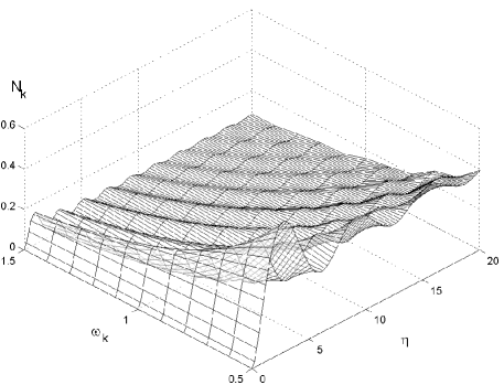
The solution of Eqs. (22)-(24) is shown at Fig. 1. In accordance with this solution, at the tremendous redshift $1+z=e^{\langle D\rangle}=a^{-1}$, $z\to\infty$, $a=0$, Eq.(20) is reduced to the zeroth mode dilaton integral of motion $\Omega_{\langle D\rangle}$ which corresponds to the z-dependence of the Hubble parameter $H(z)=H_{0}(1+z)^{2}$. At this moment, the Universe was empty, and all particle densities had the zero initial data. The same dilaton vacuum regime $H(z)=H_{0}(1+z)^{2}$ is compatible with the SNeIa data [1] in the geometry of similarity (3) [8].

The next step is the creation of gravitons induced by the direct dilaton interaction. A hypothetic observer being at the first instance at $r_{\rm I}=1/H_{\rm I}$ in the primordial volume $V_{\rm I}=4\pi r_{\rm I}^{3}/3$ observes the vacuum creation of these particles with the primordial density

$$\Omega_{g\rm I}=\omega_{\textbf{\rm c}}\cdot\frac{H^{2}_{0}}{M^{2}_{\rm Pl.}}\cdot(1+z_{\rm I})^{8}$$ (33)

defined by the Casimir energy. The question which remains to answer is how to define $z_{\rm I}$?

Figure 1: The creation of the Universe distribution $[N_{\bf k}=N_{b}]$ (27) versus dimensionless time $\eta$ and energies $0.5\leq\omega_{\bf k}$ at the initial data $N_{\bf k}(\eta=0)=0$ and the Hubble parameter $H(\eta)=1/(1+2\eta)=(1+z)^{2}$.

In order to estimate the instance of creation $(1+z_{\rm I})$, one can add the Hamiltonian of the Standard Model (SM): $\textsf{H}_{g}~{}\to~{}\textsf{H}=\textsf{H}_{g}+\textsf{H}_{\rm SM}$, – when in the limit $(1+z_{\rm I})\to\infty$ and $a\to 0$ all particles become nearly massless $\sqrt{\textbf{k}^{2}+a^{2}M^{2}_{0}}\to\omega_{\textbf{k}}$. In this case, the same mechanism of intensive particle creation works also for any scalar fields including four Higgs bosons [21]

$$\Omega_{\rm I~{}Higgs}=4\Omega_{g\rm I}.$$ (34)

The decays of the Higgs sector including longitudinal vector $W$ and $Z$ bosons approximately preserve this partial energy density for the decay products. These products are Cosmic Microwave Background (CMB) photons and $n_{\nu}$ neutrino. Therefore, one obtains

$$(1+n_{\nu})\Omega_{\rm CMB}\approx 4\Omega_{g\rm I}.$$ (35)

In our model there is the coincidence of two epochs:

• the creation of SM bosons in the Universe in electroweak epoch

  $$1+z_{\rm W}=[M_{W}/H_{0}]^{1/3}=0.37\cdot 10^{15},$$ (36)

  when the horizon $H(z_{W})=(1+z_{W})^{2}H_{0}=(1+z_{W})^{2}1.5\cdot 10^{-42}$GeV contains only a single $W$ boson;

• and the CMB origin time

  $$1+z_{\rm CMB}=[\lambda_{\rm CMB}H_{0}]^{-1/2}=[10^{-29}\cdot 2.35/1.5]^{1/2}=0.39\cdot 10^{15},$$ (37)

  when the horizon contains only a single CMB photon with mean wave length $\lambda_{\rm CMB}$ that is approximately equal to the inverse temperature $\lambda^{-1}_{\rm CMB}=T_{\rm CMB}=2.35\cdot 10^{-13}$ GeV.

In the same epoch $z_{I}\approx z_{W}\approx z_{\rm CMB}$, if the primordial graviton density (33) coincides with the CMB density normalized to a single degree of freedom (as it was supposed in [14]). The coincidence of the Planck epoch $z_{I}$ with the first two ones solves cosmological problems with the aid of the geometry of similarity (3), without the inflation (see also [8]).

While adding the SM sector to the theory in order to preserve the conformal symmetry, we should exclude the unique dimensional parameter from the SM Lagrangian, i.e. the Higgs term with a negative squared mass. However, following Kirzhnits [22], we can include the vacuum expectation of the Higgs field (its zeroth harmonic) $\langle\phi\rangle$. The latter appears as a certain external initial data or a condensate. In our construction we can choose it in the most simple form: $\langle\phi\rangle=Const=\langle\phi\rangle_{I}=246$ GeV which could be consider as the initial condition at the beginning of the Universe. The fact, that the Higgs vacuum expectation is equal to its present day value, allows us to preserve the status of the SM as the proper quantum field theory during the whole Universe evolution. The standard vacuum stability conditions

$$<0|0>|_{\phi=\langle\phi\rangle}=1,\qquad<0|0>^{\prime}|_{\phi=\langle\phi\rangle}=0$$ (38)

yield the following constraints on the Coleman–Weinberg effective potential of the Higgs field:

$$V_{\rm eff}(\langle\phi\rangle)=0,\qquad V^{\prime}_{\rm eff}(\langle\phi\rangle)=0.$$ (39)

It results in a zero contribution of the Higgs field vacuum expectation into the Universe energy density. In other words, the SM mechanism of a mass generation can be completely repeated. However, the origin of the observed conformal symmetry breaking is not a dimensional parameter of the theory but a certain non-trivial (and very simple at the same moment) set of the initial data. In particular, one obtains that the Higgs boson mass is determined from the equation $V^{\prime\prime}_{\rm eff}(\langle\phi\rangle)=M_{H}^{2}$. Note that in our construction the Universe evolution is provided by the dilaton, without making use of any special potential and/or any inflaton field. In this case we have no reason to spoil the renormalizablity of the SM by introducing the non-minimal interaction between the Higgs boson and the gravity [23].

In summary, following the ideas of the conformal symmetry [6, 7], we formulated the GR in terms of the spin-connection coefficients. The cosmological evolution of the metrics is induced by the dilaton, without the inflation hypothesis and the $\Lambda$-term. In the suggested model, the Planck epoch coincides with the thermalization and the electroweak ones. In this case the CMB power spectrum can be explained by two gamma processes of SM bosons [24], avoiding dynamical dilaton deviations with negative energy by means of the Dirac constraint (18). We have provided a few arguments in favour that the exact evolution of the GR as a theory of spontaneous conformal symmetries breaking is related to the equations for the quantum squeezed oscillator. We found that the dilaton evolution yields the vacuum creation of matter.