Landau level states on a topological insulator thin film

Abstract

We analyze the four-dimensional Hamiltonian proposed to describe the band structure of the single-Dirac-cone family of topological insulators in the presence of a uniform perpendicular magnetic field. Surface Landau level(LL) states appear, decoupled from the bulk levels and following the quantized energy dispersion of a purely two-dimensional surface Dirac Hamiltonian. A small hybridization gap splits the degeneracy of the central $n=0$ LL with dependence on the film thickness and the field strength that can be obtained analytically. Explicit calculation of the spin and charge densities show that surface LL states are localized within approximately one quintuple layer from the surface termination. Some new surface-bound LLs are shown to exist at a higher Landau level index.

I Introduction

Insulating materials with topologically protected surface states known as topological insulators (TIs) are a matter of great current interestkane-hasan ; qi-zhang ; moore . The surface metallic states in this new class of materials is characterized by Dirac-like quasiparticle dispersion, and a one-to-one correspondence between momentum and spin quantum numbers of the single-particle states thus representing an extreme form of spin-orbit coupling. Both these aspects have been confirmed for the first time in Bi_xSb_1-x familykane-fu of topological insulators by ARPESARPES-on-BiSb and STMSTM-on-BiSb studies.

More recently, a lot of experimental efforts has been given to the synthesis and characterization of Bi₂Se₃, Bi₂Te₃, and Sb₂Te₃ARPES-on-Bi2Te3 ; STM-on-Bi2Se3 ; ong ; Bi2Se3-exp ; thin-film-TI-exp-Japan ; thin-film-TI-exp-China ; STM-B-thin-film ; hanaguri following the prediction of their topological behaviorBi2Se3-theory ; Bi2Se3-theory2 , due to their simple surface band structure consisting of a single-cone Dirac spectrum centered at the $\Gamma$-point and a relatively large band gap. Topological insulators of the single-Dirac-cone family in the thin-film form has been synthesized by a number of groupsthin-film-TI-exp-Japan ; thin-film-TI-exp-China ; STM-B-thin-film . Theoretically, the thin-film TIs bear close analogy to another heavily studied topological material, i.e. graphenecastro-neto . For instance, the well-known pair of valley-degenerate Dirac bands of graphene becomes the top and bottom surface Dirac bands of TIs with finite thickness. Perpendicular magnetic field quantizes the surface Landau levels (LLs) with the energies that scale with the LL index $n$ as $\pm\sqrt{n}$ in TIs as well as in graphene.

Previous treatments of the magnetic field effect on TI surface started from the two-dimensional (2D) Dirac Hamiltonian focusing only on the surface electronic states and ignoring the bulk states altogetherqi ; SQShen-LL . These methods relied on first projecting the bulk Hamiltonian to the surface, obtaining the 2D Dirac model, then including the field effect by way of Peierls substitution. In another vein, several recent papers theoretically examined the properties of a thin slab of TI in which the bulk and surface electronic states are treated on an equal footinglinder ; liu ; shen in the absence of the magnetic field. It is thus natural to consider how the magnetic field effect plays out for a thin film geometry of TI, following the spirit of solving the bulk Hamiltonian adopted in Refs. linder, ; liu, ; shen, . In fact, an attempt of precisely this sort has been made in a recent paper by Liu et al.Bi2Se3-theory2 Here, the authors solved the $4\times 4$ tight-binding Hamiltonian with the Peierls substitution for the magnetic field and even including the Zeeman field coupling. We point out in this paper that the method adopted in Ref. Bi2Se3-theory2, does not treat the surface and bulk electronic states simultaneously, and as a result the bands arising from surface LLs penetrate into the bulk LL states, while physically such overlapping of energy levels will not occur.

Our approach follows closely the spirit of zero-field case studied in Refs. linder, ; liu, ; shen, and takes care of the boundary conditions properly. Some parts of our report are technical, dealing with the characteristic equation resulting from the boundary conditions and the methods of solving them. Several physically meaningful results follow from our analysis. First, hybridization of the zeroth-LL states localized on the top and the bottom surfaces for a sufficiently thin sample is shown to manifest itself as the splitting of the degeneracy of zeroth-LL states with the gap magnitude that can be calculated analytically. The zeroth-LL gap size oscillates with the film thickness. Our finding naturally extrapolates a similar observation of the gap oscillation observed previouslylinder to finite magnetic field. Interestingly, we find that a new kind of surface-bound LL states appear for higher-LL indices where the conventional surface LL band of $\sim\sqrt{n}$ variety has merged into the bulk continuum. Justification of the new surface LLs is made on the basis of careful numerical study and an approximate analytic solution of the characteristic equation. Properties of the bulk single-particle states for higher-LL indices are examined in detail. Finally, both charge and spin density profiles of the surface LLs at low LL indices along the thickness of the sample are explicitly worked out.

In Sec. II we formulate the LL problem based on the $4\times 4$ Hamiltonian proposed previously for Bi₂Se₃-family of topological insulators. Boundary conditions are imposed on the two surface layers for a thin-film geometry and characteristic equations are derived in Sec. III. In Sec. IV several physical results are shown and its relevance to recent STM are discussed. Summary of results and an outlook is given in Sec. V. Technical discussion for the new surface-bound LLs can be found in the Appendix.

II Formulation

The 3D tight-binding Hamiltonian proposed as a minimal model for single-Dirac-cone family of TIs first in Ref. Bi2Se3-theory, and detailed in Ref. Bi2Se3-theory2, is

$$H({\bf p})=\varepsilon({\bf p})\!+\!\begin{pmatrix}M({\bf p})\tau_{z}\!+\!A_{1}p_{z}\tau_{x}&A_{2}p_{-}\tau_{x}\\ A_{2}p_{+}\tau_{x}&M({\bf p})\tau_{z}\!-\!A_{1}p_{z}\tau_{x}\end{pmatrix}$$ (1)

in the basis spanned by $(\mathrm{Bi}^{+}_{\uparrow},\mathrm{Se}^{-}_{\uparrow},\mathrm{Bi}^{+}_{\downarrow},\mathrm{Se}^{-}_{\downarrow})$. Pauli matrices $\bm{\tau}$ are introduced and $p_{\pm}=p_{x}\pm ip_{y}$ are momentum operators. The upper and lower indices in the basis set refer to the parity and spin quantum numbers for the $p_{z}$ orbitals of Bi or Se atoms, respectively. It was shownBi2Se3-theory that $\varepsilon({\bf p})$ and $M({\bf p})$ depend on the momentum ${\bf p}$ as

$$\varepsilon({\bf p}) = C+D_{1}p_{z}^{2}+D_{2}(p_{x}^{2}+p_{y}^{2}),$$

$$M({\bf p}) = M_{0}-B_{1}p_{z}^{2}-B_{2}(p_{x}^{2}+p_{y}^{2}).$$ (2)

Values of the various constants can be found in Refs. Bi2Se3-theory, ; linder, ; liu, ; shen, ; Bi2Se3-theory2, . In our paper all the material parameters are re-scaled in terms of the one mass scale $M_{0}$. Two length parameters emerge as a result, $l_{z}=A_{1}/M_{0}$ and $l_{\perp}=A_{2}/M_{0}$, each characterizing the length scale within the plane and perpendicular to it. With the material parameters given in Ref. Bi2Se3-theory, they read $l_{\perp}=14.64$Å and $l_{z}=7.9$Å. We use them as the measure of length in each direction. All equations can be cast in dimensionless form as well as the two functions $\varepsilon({\bf p})$ and $M({\bf p})$ which now become (following the parameterization of Ref. Bi2Se3-theory, )

$$\varepsilon({\bf p}) = -0.024+0.075p_{z}^{2}+0.3265p_{\perp}^{2},$$

$$M({\bf p}) = 1-0.58p_{z}^{2}-0.94p_{\perp}^{2}.$$ (3)

Coefficient-by-coefficient, expressions in $\varepsilon({\bf p})$ are smaller than the ones in $M({\bf p})$. In this study, we will ignore $\varepsilon({\bf p})$ for calculational simplicity and restore particle-hole symmetry of the spectrum as a consequence.

The four-dimensional single-particle eigenstates can be constructed in terms of two, two-dimensional spinors $u$ and $v$. For an infinite medium one can write the eigenstate as $\psi=e^{i{\bf k}\cdot{\bf r}}\chi$, where $\chi=\begin{pmatrix}u\\ v\end{pmatrix}$ is a 4-component constant spinor to be determined by solving

$$k_{+}u = \Bigl{(}E\tau_{x}+k_{z}+iM\tau_{y}\Bigr{)}v,$$

$$k_{-}v = \Bigl{(}E\tau_{x}-k_{z}+iM\tau_{y}\Bigr{)}u,$$

$$M = 1-\alpha_{z}k_{z}^{2}-\alpha_{\perp}k_{\perp}^{2},$$ (4)

with $E$ as the energy, $k_{\pm}=k_{x}\pm ik_{y}$ as the momentum, and $\alpha_{z}$ and $\alpha_{\perp}$ are two material constants. They read $\alpha_{z}=0.58$ and $\alpha_{\perp}=0.94$ in the parametrization of Ref. Bi2Se3-theory, .

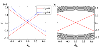
Figure 1: (color online) (a) Surface energy spectra without magnetic field when $\varepsilon_{k}=0$ (red) and $\varepsilon_{k}\neq 0$ (blue). (b) Bulk and surface energy dispersions in the absence of magnetic field and $\varepsilon_{k}=0$. $L_{z}/l_{z}$=3000 was used.

As our interest lies in the case of finite thickness $L_{z}$ for the $z$-direction the above equation will be deformed as $ik_{z}\rightarrow\lambda_{z}$linder ; liu ; shen . Due to the boundary conditions at $z=\pm L_{z}/2$, surface state solutions appearlinder ; liu ; shen . Figure 1(a) shows the difference in the surface energy spectra when the diagonal energy $\varepsilon_{k}$ is turned on/off. As stressed earlier we will suppress the diagonal energy $\varepsilon_{k}$ and work with the particle-hole symmetric model in the following section where we consider the magnetic field effect. Figure 1(b) shows the surface state energy together with the bulk energy as a function of the transverse momentum $k_{\perp}$. The edge state energy dispersion is precisely linear in $|k_{\perp}|$ for large $|k_{\perp}|$ but opens an exponentially small hybridization gap at $k_{\perp}=0$. The gap at the $\Gamma$-point is given byshen

$$\Delta = {8\alpha\over\beta}\ e^{-\alpha L_{z}}|\sin(\beta L_{z})|,$$ (5)

where $\alpha$, $\beta$ are

$$\alpha={1\over 2\alpha_{z}},~{}~{}\beta={\sqrt{4\alpha_{z}-1}\over 2\alpha_{z}}.$$ (6)

This result will be generalized in the following section to the nonzero magnetic field, with the revised meaning for the gap as the energy difference of symmetric and anti-symmetric combinations of zeroth-Landau levels localized to top and bottom surface layers.

III Landau Levels

Magnetic field ${\bf H}=(0,0,H)$ perpendicular to the slab modifies the momentum operator ${\bf p}\rightarrow{\bf p}+{\bf A}=(p_{x}-Hy,p_{y},p_{z})$ in the Hamiltonian. A pair of canonical operators

$$\mathcal{A}={1\over\sqrt{2}}\Bigl{(}{y\!-\!y_{0}\over l_{H}}\!+\!l_{H}\partial_{y}\Bigr{)},~{}\mathcal{A}^{\dagger}={1\over\sqrt{2}}\Bigl{(}{y\!-\!y_{0}\over l_{H}}\!-\!l_{H}\partial_{y}\Bigr{)},$$ (7)

are introduced such that $[\mathcal{A},\mathcal{A}^{\dagger}]=1$. The magnetic length (measured in units of $l_{\perp}$) appears as $l_{H}=1/\sqrt{H}$, as well as the guiding center $y_{0}=l_{H}^{2}k_{x}$. Relation to the physical field strength $H_{\mathrm{phys}}$ in Tesla is

$$H={l_{\perp}^{2}eH_{\mathrm{phys}}/\hbar}\simeq 3.25\times 10^{-3}H_{\mathrm{phys}}/[\mathrm{T}].$$ (8)

Taking $k_{+}=-(\sqrt{2}/l_{H})\mathcal{A}^{\dagger}$ and $k_{-}=-(\sqrt{2}/l_{H})\mathcal{A}$, the eigenvalue equation for a slab with perpendicular magnetic field becomes

$$\mathcal{A}^{\dagger}u = -{l_{H}\over\sqrt{2}}\Bigl{(}E\tau_{x}-i\lambda_{z}+iM_{\hat{N}}\tau_{y}\Bigr{)}v,$$

$$\mathcal{A}v = -{l_{H}\over\sqrt{2}}\Bigl{(}E\tau_{x}+i\lambda_{z}+iM_{\hat{N}}\tau_{y}\Bigr{)}u,$$ (9)

with several new definitions ($\hat{N}=\mathcal{A}^{\dagger}\mathcal{A}$)

$$\alpha_{H}={2\alpha_{\perp}\over l_{H}^{2}},~{}~{}M_{\hat{N}}=1+\alpha_{z}\lambda_{z}^{2}-\alpha_{H}\Bigl{(}\hat{N}+{1\over 2}\Bigr{)}.$$ (10)

The rest of this section is concerned with the solution of this equation, together with the boundary conditions at the two terminations $z=\pm L_{z}/2$.

The structure of the equation invites for a solution of the form $u=\phi_{n-1}\begin{pmatrix}a_{n}\\ b_{n}\end{pmatrix}$, and $v=\phi_{n}\begin{pmatrix}c_{n}\\ d_{n}\end{pmatrix}$, where $\phi_{n}$ is the $n$-th Landau level (LL) oscillator wave function centered at $y=y_{0}$. By substituting the ansatz to Eq. (9) we getcomment

$$\sqrt{n}\begin{pmatrix}a_{n}\\ b_{n}\end{pmatrix}=-{l_{H}\over\sqrt{2}}\Bigl{(}E\tau_{x}\!-\!i\lambda_{z}\!+\!iM_{n}\tau_{y}\Bigr{)}\begin{pmatrix}c_{n}\\ d_{n}\end{pmatrix},$$

$$\sqrt{n}\begin{pmatrix}c_{n}\\ d_{n}\end{pmatrix}=-{l_{H}\over\sqrt{2}}\Bigl{(}E\tau_{x}\!+\!i\lambda_{z}\!+\!iM_{n-1}\tau_{y}\Bigr{)}\begin{pmatrix}a_{n}\\ b_{n}\end{pmatrix},$$

$$M_{n}=1+\alpha_{z}\lambda_{z}^{2}-\alpha_{H}\Bigl{(}n+{1\over 2}\Bigr{)}.$$ (11)

We can parameterize the spinor solution $u$ and $v$ satisfying Eq. (11) in the following form

$$u=\phi_{n-1}\cos\varphi\begin{pmatrix}-i\sin{\theta}\\ \cos{\theta}\end{pmatrix},~{}~{}v=\phi_{n}\sin\varphi\begin{pmatrix}\cos{\theta}\\ i\sin{\theta}\end{pmatrix}$$ (12)

with the two complex angles $(\theta,\varphi)$ fixed by

$$\tan{\theta}={\lambda_{z}\over E+\mu},~{}~{}~{}\tan\varphi=-{{M_{n-1}\!+\!\mu}\over{\sqrt{2n}/l_{H}}}.$$ (13)

Here $\mu$ means

$$\mu\alpha_{H}=M_{n}^{2}-E^{2}-\lambda_{z}^{2}+\alpha_{H}M_{n}+{2n\over l_{H}^{2}}.$$ (14)

The eigenvalues are fixed up by the relation $\mu^{2}=E^{2}+\lambda_{z}^{2}$ which reads when $\mu$ is explicitly written out

$$\left(M_{n}^{2}\!-\!E^{2}\!-\!\lambda_{z}^{2}+\alpha_{H}M_{n}\!+\!{2n\over l_{H}^{2}}\right)^{2}=\alpha_{H}^{2}(E^{2}\!+\!\lambda_{z}^{2}).$$ (15)

This is the desired characteristic equation for the energy $E$.

Being eighth-power in $\lambda_{z}$, one can find eight different $\lambda_{z}$’s for a given energy. We call them $a\lambda_{b}$ as in the non-magnetic caselinder ; liu ; shen , with $a=\pm$ and $b=1,2,3,4$. There are thus eight independent solutions of the same energy $E$ for a given LL index $n$ and the guiding center $y_{0}$,

$$\chi_{nab}(y\!-\!y_{0}) = \begin{pmatrix}-ia\sin{\theta_{b}}\cos\varphi_{b}\phi_{n-1}\\ \cos{\theta_{b}}\cos\varphi_{b}\phi_{n-1}\\ \cos{\theta_{b}}\sin\varphi_{b}\phi_{n}\\ ia\sin{\theta_{b}}\sin\varphi_{b}\phi_{n}\end{pmatrix}.$$ (16)

Taking the linear combination among the eight states gives out the most general eigenstate before the boundary condition is imposed as

$$\psi_{nk_{x}}(x,y-y_{0},z)=e^{ik_{x}x}\sum_{ab}A_{ab}e^{a\lambda_{b}z}\chi_{nab}(y-y_{0}).$$ (17)

To facilitate the further solution, the coefficients $A_{ab}$ can be classified into symmetric ($A_{ab}=A_{b}$) and anti-symmetric ($A_{ab}=aA_{b}$) types. For the symmetric case the boundary conditions at $z=\pm L_{z}/2$, $\psi_{nk_{x}}(x,y-y_{0},L_{z}/2)=\psi_{nk_{x}}(x,y-y_{0},-L_{z}/2)=0$, can be satisfied if we require that $A_{b}$ obey

$$\sum_{b}A_{b}\sinh(\lambda_{b}L_{z}/2)\sin{\theta_{b}}\sin\varphi_{b}=0,$$

$$\sum_{b}A_{b}\sinh(\lambda_{b}L_{z}/2)\sin{\theta_{b}}\cos\varphi_{b}=0,$$

$$\sum_{b}A_{b}\cosh(\lambda_{b}L_{z}/2)\cos{\theta_{b}}\sin\varphi_{b}=0,$$

$$\sum_{b}A_{b}\cosh(\lambda_{b}L_{z}/2)\cos{\theta_{b}}\cos\varphi_{b}=0.$$ (18)

A nontrivial solution exists provided the characteristic equation of the above 4$\times$4 matrix is zero. With the aid of Eq. (13) this condition can be expressed as

$$\Bigl{(}{\lambda_{1}\lambda_{2}\tanh{\lambda_{1}L_{z}\over 2}\tanh{\lambda_{2}L_{z}\over 2}\over(E_{n}\!+\!\mu_{n,1})(E_{n}\!+\!\mu_{n,2})}+{\lambda_{3}\lambda_{4}\tanh{\lambda_{3}L_{z}\over 2}\tanh{\lambda_{4}L_{z}\over 2}\over(E_{n}\!+\!\mu_{n,3})(E_{n}\!+\!\mu_{n,4})}\Bigr{)}(\mu_{n,1}\!-\!\mu_{n,2}\!+\alpha_{z}(\lambda_{1}^{2}-\lambda_{2}^{2}))(\mu_{n,3}\!-\!\mu_{n,4}\!+\alpha_{z}(\lambda_{3}^{2}-\lambda_{4}^{2}))$$

$$+ \Bigl{(}{\lambda_{1}\lambda_{4}\tanh{\lambda_{1}L_{z}\over 2}\tanh{\lambda_{4}L_{z}\over 2}\over(E_{n}+\mu_{n,1})(E_{n}+\mu_{n,4})}+{\lambda_{2}\lambda_{3}\tanh{\lambda_{2}L_{z}\over 2}\tanh{\lambda_{3}L_{z}\over 2}\over(E_{n}\!+\!\mu_{n,2})(E_{n}\!+\!\mu_{n,3})}\Bigr{)}(\mu_{n,1}\!-\!\mu_{n,4}\!+\alpha_{z}(\lambda_{1}^{2}-\lambda_{4}^{2}))(\mu_{n,2}\!-\!\mu_{n,3}\!+\alpha_{z}(\lambda_{2}^{2}-\lambda_{3}^{2}))$$

$$= \Bigl{(}{\lambda_{1}\lambda_{3}\tanh{\lambda_{1}L_{z}\over 2}\tanh{\lambda_{3}L_{z}\over 2}\over(E_{n}+\mu_{n,1})(E_{n}\!+\!\mu_{n,3})}+{\lambda_{2}\lambda_{4}\tanh{\lambda_{2}L_{z}\over 2}\tanh{\lambda_{4}L_{z}\over 2}\over(E_{n}\!+\!\mu_{n,2})(E_{n}\!+\!\mu_{n,4})}\Bigr{)}(\mu_{n,1}\!-\!\mu_{n,3}\!+\alpha_{z}(\lambda_{1}^{2}-\lambda_{3}^{2}))(\mu_{n,2}\!-\!\mu_{n,4}\!+\alpha_{z}(\lambda_{2}^{2}-\lambda_{4}^{2})),$$

where $M_{n,b}=1+\alpha_{z}\lambda_{b}^{2}-\alpha_{H}(n+1/2)$, and $\mu_{n,b}\alpha_{H}=M_{n,b}^{2}-E_{n}^{2}-\lambda_{b}^{2}+\alpha_{H}M_{n,b}+2n/l_{H}^{2}$.

The case of anti-symmetric coefficients $A_{ab}=aA_{b}$ can be handled by interchanging $\sinh(\lambda_{b}L_{z}/2)$ and $\cosh(\lambda_{b}L_{z}/2)$ in Eq. (18), and replacing $\tanh(\lambda_{b}L_{z}/2)$ by $\coth(\lambda_{b}L_{z}/2)$ in Eq. (LABEL:eq:char-eq-for-LL). Equation (LABEL:eq:char-eq-for-LL) and its anti-symmetric counterpart can be solved numerically for given $n$, giving out simultaneously surface and bulk energy solutions in the presence of the field $H$. When $L_{z}$ becomes large both $\tanh(\lambda_{b}L_{z}/2)$ and $\coth(\lambda_{b}L_{z}/2)$ tend to the same value and we will have a pair of degenerate states for each energy, each state being localized either at the top or the bottom surface and not coupled to the opposite layer.

The zeroth-LL $n=0$ requires a separate treatment. In this case $u$ is identically zero, and $v^{T}=(c_{0},d_{0})$ is found from solving

$$-{l_{H}\over\sqrt{2}}\Bigl{(}E\tau_{x}\!-\!i\lambda_{z}\!+\!iM_{0}\tau_{y}\Bigr{)}\begin{pmatrix}c_{0}\\ d_{0}\end{pmatrix}=0,$$ (20)

with $M_{0}=1+\alpha_{z}\lambda_{z}^{2}-\alpha_{H}/2$. For a given energy $E_{0}$, $E_{0}^{2}=M_{0}^{2}-\lambda_{z}^{2}$ results in four different $\lambda_{z}$’s, $a\lambda_{b}$ with $a=\pm$ and $b=1,2$. Similar to Eq. (16) one can assume the spinor solution for $n=0$

$$\chi_{0ab}(y-y_{0})=\phi_{0}(y-y_{0})\begin{pmatrix}0\\ 0\\ \cos\theta_{b}\\ ia\sin\theta_{b}\end{pmatrix}$$ (21)

where $\theta_{b}$ is given by

$$\tan\theta_{b}={\lambda_{b}\over E+M_{0,b}},$$ (22)

and

$$M_{0,b} = 1+\alpha_{z}\lambda_{b}^{2}-\alpha_{H}/2,$$

$$\lambda_{b} = {1\over\sqrt{2}\alpha_{z}}\Bigl{(}1-2\alpha_{z}+\alpha_{\perp}^{\prime}\alpha_{z}$$ (23)

$$-(-1)^{b}\sqrt{1-4\alpha_{z}+2\alpha_{H}\alpha_{z}+4E^{2}\alpha_{z}^{2}}\Bigr{)}^{{1\over 2}}.$$

A linear combination

$$\psi_{0k_{x}}(y-y_{0})=\sum_{ab}A_{ab}e^{a\lambda_{b}z}\chi_{0ab}(y-y_{0})$$ (24)

can be formed with the boundary conditions at $z=\pm L_{z}/2$. Again assuming symmetric ($A_{ab}=A_{b}$) and anti-symmetric ($A_{ab}=aA_{b}$) coefficients separately and denoting the corresponding energies by $E_{0}^{S}$ and $E_{0}^{A}$, we have

$${\lambda_{2}\over\lambda_{1}}{E_{0}^{S}\!+\!M_{0,1}\over E_{0}^{S}\!+\!M_{0,2}} = {\tanh{\lambda_{1}L_{z}\over 2}\over\tanh{\lambda_{2}L_{z}\over 2}},$$ (25)

and

$${\lambda_{2}\over\lambda_{1}}{E_{0}^{A}\!+\!M_{0,1}\over E_{0}^{A}\!+\!M_{0,2}} = {\tanh{\lambda_{2}L_{z}\over 2}\over\tanh{\lambda_{1}L_{z}\over 2}}.$$ (26)

One can easily show from Eqs. (25) and (26) that $E_{0}^{A}=-E_{0}^{S}$.

This completes the derivation of the full energy spectra and eigenstates for a thin-slab geometry of TI model with the perpendicular magnetic field. In the following section we discuss several physical results obtained from the analysis of the solution.

IV Physical Results

Figure 2 shows the dependence of surface and bulk energies on the LL index $n$, for a sufficiently large thickness $L_{z}$. The numerical results remain consistently similar for $L_{z}$ larger than about ten times $l_{z}$. A most surprising aspect of the numerical analysis is the existence of three distinct branches of surface-localized states, labeled as (I), (II), and (III) in Fig. 2.

The behavior of the first surface branch $E^{(1)}_{n}$ is remarkably close to the formula:

$$E^{(s)}_{n}\simeq\pm\sqrt{2n}/l_{H}=\pm\sqrt{2nH}.$$ (27)

This is exactly what is expected of the purely two-dimensional Dirac Hamiltonian with the Fermi velocity $v_{F}=1$ (equal to $M_{0}l_{\perp}/\hbar=A_{2}/\hbar\approx 6.2\times 10^{5}$ m/s in physical units)Bi2Se3-theory . Restoring all physical units, the surface LLs occur at

$$E^{(s)}_{n}=\pm{A_{2}\over l_{H_{\mathrm{phys}}}}\sqrt{2n}.$$ (28)

Physical magnetic field $H_{\mathrm{phys}}=11$T results in the magnetic length $l_{H_{\mathrm{phys}}}=\sqrt{\hbar/eH_{\mathrm{phys}}}\sim 100$Å  and the energy levels $\pm 58\sqrt{n}$ mV. Indeed the spacing in the $n=0$ and $n=1$ LL peaks were found to be about $40\sim 50$ mVSTM-B-thin-film .

Using the physical magnetic field $H_{\mathrm{phys}}=10$T we find that at $n>n_{c}\approx 12$ the first branch of surface LL begins to merge with the bulk spectrum (Fig. 2). Here $n_{c}$ corresponds to the Landau level index for which the surface LL begins to touch the bottom of the bulk band. A sharper criterion to determine $n_{c}$ can be drawn by keeping track of the eigenvalues $\lambda_{b}$ for the surface-bound LLs. With increasing $n$, one of the four $\lambda_{b}$’s forming the surface LL eigenstate has its real part decrease and eventually touch zero at $n=n_{c}$. This signals the mixture of an extended state in the wave function just as the surface LL merges with the bulk continuum. Recently, the number of surface LLs that can be resolved in the tunneling spectra of STMSTM-B-thin-film was shown to be about 12, consistent with our estimate of $n_{c}$. For $n>n_{c}$, the surface branch no longer exists independently of the bulk LL, but rather seems to form the bottom of the bulk band as depicted in Fig. 2.

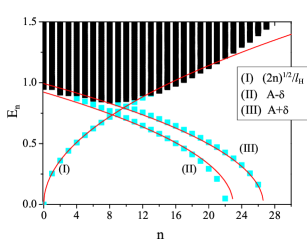
Figure 2: (color online) Landau level energies for $L_{z}/l_{z}=3\times 30^{3}$ and H_phys=10T, showing both surface(sky blue square) and bulk states(black square). Three surface branches are labeled (I) through (III) with analytic fits shown as red solid curves to $\sqrt{2n}/l_{H}$ (branch I) and $\sqrt{A\pm\delta-Bn}$ (branches II and III). $A$ and $B$ values are derived in the Appendix and a small offset $\delta$ is used to fit the numerical results. When H_phys=10T, $A=0.918,~{}\delta=0.068,~{}B=0.037$, respectively.

A recent paper by Liu et al. also computed the bulk and surface LLs based on the model Hamiltonian for Bi₂Se₃. In their Fig. 7 it appeared as though the surface LLs can exist well inside the bulk spectra as an independent branch. We believe this is an artifact of their calculation not taking care of the boundary conditions precisely. Once the boundary conditions at $z=\pm L_{z}/2$ are handled properly, the correct energy profile for $n>n_{c}$ is the one in which the surface-localized wave functions are hybridized with the extended states to form a “hybrid” state. To confirm this assertion, we have made a careful analysis of all the $\lambda_{b}$ values for eigenstates with energies both at the bottom of, and deep inside the bulk for $n>n_{c}$. While the details are too tedious to report here, we can say with certainty that states forming the bulk LL are typically a linear combination of solutions with real $\lambda_{b}$ (localized to surface) and some with purely imaginary $\lambda_{b}$ (extended). See Eq. (17) for a general definition of the eigenstate. Only for the three surface branches (I) through (III) is it possible to get all $\lambda_{b}$’s of the eigenstate being real and the wave function completely localized.

The existence of extra two surface branches, labeled (II) and (III) in Fig. 2, is unexpected. They begin to appear at $n\approx 4$ and $n\approx 8$ respectively for $H_{\mathrm{phys}}=10$T. We have confirmed their existence for $L_{z}/l_{z}$ as small as 10 and as large as 3000. Due to the insensitivity of their features to surface thickness, we can first of all conclude that the extra surface modes are bound to one particular surface and not hybridized with the other one. To further confirm that these branches are genuine, we have carried out an approximate analytic treatment valid at large LL index $n$ and infinite thickness $L_{z}$ and indeed found that two extra branches exist. Details of this analysis are given in the Appendix.

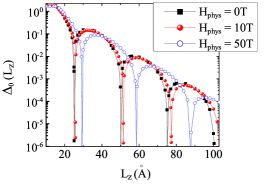
Figure 3: (color online) Hybridization gap energies for $H_{\mathrm{phys}}=0$T, 10T, and 50T with varying thickness $L_{z}$.

Hybridization effect mixes the two degenerate $n=0$ LLs previously associated with each surface layer and opens a gap. We have derived the $n=0$ surface LL energies analytically for symmetric $(E^{S}_{0})$ and anti-symmetric ($E^{A}_{0}$) combinations as

$$E_{0}^{S} \simeq -{4\alpha(H)\over\beta(H)}(1\!-\!\alpha_{\perp}H)\sin[\beta(H)L_{z}]e^{-\alpha(H)L_{z}},$$ (29)

and $E_{0}^{A}=-E_{0}^{S}$. The gap is defined as $\Delta_{0}=|E_{0}^{S}-E_{0}^{A}|=2|E_{0}^{S}|$. For practically available field strengths where $H\ll 1$, $\alpha(H)$ and $\beta(H)$ in Eq. (29) are

$$\alpha(H)\simeq{1\over 2\alpha_{z}},~{}~{}\beta(H)\simeq{\sqrt{4\alpha_{z}\!-\!1\!-\!4\alpha_{z}\alpha_{\perp}H}\over 2\alpha_{z}}.$$ (30)

They reduce exactly to $\alpha$ and $\beta$ coefficients obtained in Eq. (6) as $H\rightarrow 0$. The gap still exhibits an oscillatory decay similar to the gap at the $\Gamma$-point without magnetic field. In Fig. 3 we compare the energy gaps for zero-field and for $H_{\mathrm{phys}}=10$T and 50T. The similarity of their $L_{z}$-dependence is a strong clue that the origins of the gaps are the same. Ignoring the small field-induced shift, the gap can be

$$\Delta_{0}\approx 7M_{0}e^{-L_{z}/[9.2\AA]}\approx 2e^{-L_{z}/[9.2\AA]}\mathrm{eV}.$$ (31)

It gives a value $\approx 10$ meV for a seven quintuple-layer thin film and may well be resolved as two split $n=0$ LLs in a careful STM spectroscopy study. Currently available thin-film STM study was done on 50 quintuple-layer sampleSTM-B-thin-film . In Ref. liu, it was argued that the oscillation in the sign of the hybridization gap under zero magnetic field marks the transition between topologically trivial and non-trivial insulator phases. If this is so, our calculation seems to reveal that well-defined Dirac-like LLs exists regardless of the thickness and the sign of the gap, implying that changes in the topological character of the thin-film TI will not be revealed by examination of the surface LLs alone.

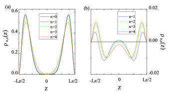
Figure 4: (color online) $n$th-LL wave function density $\rho_{n,c}(z)$ and the spin density $\rho_{n,s}(z)$for $L_{z}=60$Å.

The charge $(c)$ and spin $(s)$ densities of each $n$-th surface LL wave function can be defined as

$$\rho_{n,s(c)}(z) = {\int dxdy~{}\psi^{\dagger}_{n}\Gamma_{s(c)}\psi_{n}\over\int dxdydz~{}\psi^{\dagger}_{n}\psi_{n}},$$

$$\Gamma_{s} = \mathrm{diag}(1,1,-1,-1),$$

$$\Gamma_{c} = \mathrm{diag}(1,1,1,1).$$ (32)

Figure 4 shows results for a few surface LLs with small LL index $n$. All surface LLs are localized to within one $l_{z}$ of the termination, or within about one quintuple layer. As one can see from Fig. 4(b), the zeroth-LL is completely spin-polarized, $\int\rho_{0,s}(z)dz=-1$, while other higher surface LLs are nearly spin-quenched, $\int\rho_{n>0,s}(z)dz\approx 0$. The zeroth-LL has only the lower two elements of the four-component spinor $\chi$ take nonzero values, which refer to the amplitudes for Bi and Se states of spin-$\downarrow$ (See text following Eq. 1). There are two $n=0$ LL in the solution, and both of them are fully spin-$\downarrow$-polarized. The origin of the spin polarization is the analogue of the sublattice polarization of the $n=0$ LL in graphenecastro-neto . The difference is that the two valley $n=0$ Landau levels occupy the opposite sublattices, so that the overall sublattice symmetry is restored.

Here, by contrast, both top and bottom surface LLs give the same spin polarization. The reason is that for the top surface Dirac states the magnetic field is pointing out of the bulk but the bottom surface states experience the field pointing into the bulk, so that effectively the sense of the field direction is also reversed between the two surface layers. By reversing the field direction from $+\hat{z}$ to $-\hat{z}$ one will generate $n=0$ of spin-$\uparrow$ polarization. As a result a thin slab of TI subject to quantizing magnetic field creates two $n=0$ LLs which are completely spin polarized. Such spin-polarized surface layers are detectable by Faraday or Kerr rotation experimentsBi2Se3-theory .

V Conclusion

We showed how to derive the Landau level solution for a slab geometry of the topological insulator based on the four-band modelBi2Se3-theory ; Bi2Se3-theory2 . Previoius approaches were to first project the zero-field bulk Hamiltonian to the surface, then using the Peierls substitution to address the magnetic field effectSQShen-LL ; Bi2Se3-theory2 . Our strategy by contrast is to introduce the Peierls substitution directly into the bulk Hamiltonian and use the boundary conditions appropriate for a slab geometry. The obtained surface Landau level energies are in good accord with those obtained from the surface Dirac Hamiltonian, and we conclude that surface projection and the Peierls substitution can be implemented in any order with the same physical spectrum.

A dramatic departure of the present Dirac LL problem with an analogous one posed by the graphene systemcastro-neto is that the surface LLs are eventually bounded by the bulk spectra, and one has to face the issue what will happen to the surface LLs as they begin to merge with the bulk continuum. We addressed such a question numerically and analytically in this paper, with a prediction for the existence of new surface-bound LLs appearing at higher-LL indices. Detection of the predicted new surface modes presents an interesting challenge for the future surface-sensitive measurements on TI materials.

Appendix A Analysis of New Surface Modes

After some trial and error, we find that the following ansatz describe the numerically found surface modes (2) and (3) with good accuracy.

$$\lambda_{b}^{2}={\alpha_{H}\over\alpha_{z}}(n-m_{b}\sqrt{n}).$$ (33)

Here $m_{b}$ is a constant, to be determined later. This gives for $M_{n}$,

$$M_{n}=1-\alpha_{H}m_{b}\sqrt{n}-{1\over 2}\alpha_{H}.$$ (34)

We can also make an ansatz for the surface energy mode of the form

$$E_{n}^{2}=A-Bn,$$ (35)

with two undetermined positive coefficients $A$ and $B$. Inserting Eqs. (33) through (35) into Eq. (15) gives

$$\left[\left({\alpha^{2}_{H}}m_{b}^{2}+B-{\alpha_{H}\over\alpha_{z}}+{2\over l_{H}^{2}}\right)n+\left({1\over\alpha_{z}}-2\right)\alpha_{H}m_{b}\sqrt{n}+\cdots\right]^{2}=\alpha_{H}^{2}\left({\alpha_{H}\over\alpha_{z}}-B\right)n+\cdots.$$ (36)

The terms in $\cdots$ have subleading order in $n$ than the ones shown. Assuming a sufficiently large $n$ we require that the two sides of the equation cancel out at each order in $n$. From the equality of $n^{2}$, $n$, and $\sqrt{n}$-order terms we obtain the three following equations:

$$(\alpha_{H}m_{b})^{2} = {\alpha_{H}\over\alpha_{z}}-{2\over l_{H}^{2}}-B,$$

$$\left({1\over\alpha_{z}}-2\right)^{2}(\alpha_{H}m_{b})^{2} = \alpha_{H}^{2}\left({\alpha_{H}\over\alpha_{z}}-B\right),$$

$$2(1-{\alpha_{H}^{2}\over 4}-A)({1\over\alpha_{z}}-2)\alpha_{H}^{2}m_{b} = -{\alpha_{H}\over\alpha_{z}}\alpha_{H}^{2}m_{b}.$$ (37)

Upon solving them we obtain

$$m_{b}^{2} = {2/l_{H}^{2}\over(2-1/\alpha_{z})^{2}-\alpha_{H}^{2}},$$

$$B = {2\over l_{H}^{2}}-{\alpha_{H}\over\alpha_{z}}-{2\alpha_{H}^{2}/l_{H}^{2}\over(2-1/\alpha_{z})^{2}-\alpha_{H}^{2}},$$

$$A = 1-{\alpha_{H}^{2}\over 4}+{2\alpha_{H}^{2}/\alpha_{z}\over 1/\alpha_{z}-2}.$$ (38)

Further consideration of sub-leading corrections finally yield a splitting of $A$ into two branches responsible for (II) and (III) in Fig. 2. Rather than going into the complicated sub-leading order analysis, we can simply split $A$ into two branches by writing $A\pm\delta$ with $\delta$ chosen to fit the two branches in Fig. 2 while $A$ itself is completely determined from the parameters such as $\alpha_{z}$ and $\alpha_{\perp}$. It is shown that both branches (II) and (III) match quite well the ansatz for energy, Eq. (35).

We can also discuss the stability of the new surface branches by recalling the numerical value $\alpha_{z}=0.58$, and $\alpha_{H}=2\alpha_{\perp}/l_{H}^{2}=1.84/l_{H}^{2}$. It follows that positive $(\alpha_{H}m_{b})^{2}$ is possible if $2-(0.58)^{-1}-1.84/l_{H}^{2}=0.276-1.84/l_{H}^{2}>0$, or if $l_{H}^{2}>6.66$. Returning to physical length scales, this implies the magnetic length greater than $\sim$38Å, or the magnetic field strength less than 46T. We then expect that surface modes (II) and (III) should co-exist with the more familiar mode (I) inside the bulk gap for typical laboratory magnetic field ranges.

References

- (1) M. Z. Hasan and C. L. Kane, Rev. Mod. Phys. 82, 3045 (2010).
- (2) X.-L. Qi and S.-C. Zhang, Physics Today 63, 33 (2010).
- (3) Joel E. Moore, Nature 464, 194 (2010).
- (4) L. Fu and C. L. Kane, Phys. Rev. B 76, 045302 (2007).
- (5) D. Hsieh, D. Qian, L. Wray, Y. Xia, Y. S. Hor, R. J. Cava, and M. Z. Hasan, Nature 452, 970 (2008); D. Hsieh, Y. Xia, L. Wray, D. Qian, A. Pal, J. H. Dil, J. Osterwalder, F. Meier, G. Bihlmayer, C. L. Kane, Y. S. Hor, R. J. Cava, and M. Z. Hasan, Science 323, 919 (2009).
- (6) Pedram Roushan, Jungpil Seo, Colin V. Parker, Y. S. Hor, D. Hsieh, Dong Qian, Anthony Richardella, M. Z. Hasan, R. J. Cava and Ali Yazdani, Nature 460, 1106 (2009).
- (7) Y. Xia, D. Qian, D. Hsieh, L.Wray, A. Pal, H. Lin, A. Bansil, D. Grauer, Y. S. Hor, R. J. Cava and M. Z. Hasan, Nat. Phys. 5, 398 (2009); D. Hsieh, Y. Xia, D. Qian, L. Wray, J. H. Dil, F. Meier, J. Osterwalder, L. Patthey, J. G. Checkelsky, N. P. Ong, A. V. Fedorov, H. Lin, A. Bansil, D. Grauer, Y. S. Hor, R. J. Cava, and M. Z. Hasan, Nature 460, 1101 (2009); D. Hsieh, Y. Xia, D. Qian, L. Wray, F. Meier, J. H. Dil, J. Osterwalder, L. Patthey, A. V. Fedorov, H. Lin, A. Bansil, D. Grauer, Y. S. Hor, R. J. Cava, and M. Z. Hasan, Phys. Rev. Lett. 103, 146401 (2009); Y. L. Chen, J. G. Analytis, J.-H. Chu, Z. K. Liu, S.-K. Mo, X. L. Qi, H. J. Zhang, D. H. Lu, X. Dai, Z. Fang, S. C. Zhang, I. R. Fisher, Z. Hussain, and Z.-X. Shen, Science 325, 178 (2009).
- (8) J. G. Checkelsky, Y. S. Hor, M.-H. Liu, D.-X. Qu, R. J. Cava, and N. P. Ong, Phys. Rev. Lett. 103, 246601 (2009); J. G. Checkelsky, Y. S. Hor, R. J. Cava and N. P. Ong, arXiv:1003.3883v1 (2010).
- (9) Kazuma Eto, Zhi Ren, A. A. Taskin, Kouji Segawa, and Yoichi Ando, Phys. Rev. B 81, 195309 (2010); James G. Analytis, Jiun-Haw Chu, Yulin Chen, Felipe Corredor, Ross D. McDonald, Z. X. Shen, and Ian R. Fisher, Phys. Rev. B 81, 205407 (2010); N. P. Butch, K. Kirshenbaum, P. Syers, A. B. Sushkov, G. S. Jenkins, H. D. Drew, and J. Paglione, Phys. Rev. B 81, 241301(R) (2010).
- (10) Tong Zhang, Peng Cheng, Xi Chen, Jin-Feng Jia, Xucun Ma, Ke He, Lili Wang, Haijun Zhang, Xi Dai, Zhong Fang, Xincheng Xie, and Qi-Kun Xue, Phys. Rev. Lett. 103, 266803 (2009); Zhanybek Alpichshev, J. G. Analytis, J.-H. Chu, I. R. Fisher, Y. L. Chen, Z. X. Shen, A. Fang, and A. Kapitulnik, Phys. Rev. Lett. 104, 016401 (2010).
- (11) Yusuke Sakamoto, Toru Hirahara, Hidetoshi Miyazaki, Shin-ichi Kimura, and Shuji Hasegawa, Phys. Rev. B 81, 165432 (2010).
- (12) Guanhua Zhang, Huajun Qin, Jing Teng, Jiandong Guo, Qinlin Guo, Xi Dai, Zhong Fang, and Kehui Wu, Appl. Phys. Lett. 95, 053114 (2009); Yi Zhang, Ke He, Cui-Zu Chang, Can-Li Song, Li-LiWang, Xi Chen, Jin-Feng Jia, Zhong Fang, Xi Dai, Wen-Yu Shan, Shun-Qing Shen, Qian Niu, Xiao-Liang Qi, Shou-Cheng Zhang, Xu-Cun Ma and Qi-Kun Xue, Nat. Phys. 6, 584 (2010).
- (13) Peng Cheng, Canli Song, Tong Zhang, Yanyi Zhang, Yilin Wang, Jin-Feng Jia, Jing Wang, Yayu Wang, Bang-Fen Zhu, Xi Chen, Xucun Ma, Ke He, Lili Wang, Xi Dai, Zhong Fang, X. C. Xie, Xiao-Liang Qi, Chao-Xing Liu, Shou-Cheng Zhang, and Qi-Kun Xue, Phys. Rev. Lett. 105, 076801 (2010).
- (14) T. Hanaguri, K. Igarashi, M. Kawamura, H. Takagi, and T. Sasagawa, Phys. Rev. B 82, 081305(R) (2010).
- (15) Haijun Zhang, Chao-Xing Liu, Xiao-Liang Qi, Xi Dai, Zhong Fang and Shou-Cheng Zhang, Nat. Phys. 5, 438 (2009).
- (16) Chao-Xing Liu, Xiao-Liang Qi, HaiJun Zhang, Xi Dai, Zhong Fang, and Shou-Cheng Zhang, Phys. Rev. B 82, 045122 (2010).
- (17) A. H. Castro Neto, F. Guinea, N. M. R. Peres, K. S. Novoselov, and A. K. Geim, Rev. Mod. Phys. 81, 109 (2009).
- (18) Xiao-Liang Qi, Taylor L. Hughes, and Shou-Cheng Zhang, Phys. Rev. B 78, 195424 (2008).
- (19) Shun-Qing Shen, arXiv:0909.4125 (2009).
- (20) Jacob Linder, Takehito Yokohama, and Asle Sudbø, Phys. Rev. B 80, 205401 (2009).
- (21) Chao-Xing Liu, Haijun Zhang, Binghai Yan, Xiao-Liang Qi, Thomas Frauenheim, Xi Dai, Zhong Fang, and Shou-Cheng Zhang, Phys. Rev. B 81, 041307(R) (2010).
- (22) Hai-Zhou Lu, Wen-Yu Shan, Wang Yao, Qian Niu, and Shun-Qing Shen, Phys. Rev. B 81, 115407 (2010); Wen-Yu Shan, Hai-Zhou Li, and Shun-Qing Shen, New J. Phys. 12, 043048 (2010).
- (23) It follows immediately that an eigenstate with energy is obtained from the state with energy in Eq. (9) by the operation .