Directed motion of domain walls in biaxial ferromagnets under the influence of periodic external magnetic fields

Abstract

Directed motion of domain walls (DWs) in a classical biaxial ferromagnet placed under the influence of periodic unbiased external magnetic fields is investigated. Using the symmetry approach developed in this article the necessary conditions for the directed DW motion are found. This motion turns out to be possible if the magnetic field is applied along the easiest axis. The symmetry approach prohibits the directed DW motion if the magnetic field is applied along any of the hard axes. With the help of the soliton perturbation theory and numerical simulations, the average DW velocity as a function of different system parameters such as damping constant, amplitude, and frequency of the external field, is computed.

1 Introduction

One-dimensional ferromagnetic models are currently of considerable experimental and theoretical interest kik90pr ; ms91adp . A large portion of this interest has been directed towards the domain wall (DW) response to an ac magnetic field. One of the important problems here is the development of different ways for obtaining a net DW drift under the influence of unbiased perturbations.

The ratchet effect jap97rmp ; r02pr ; hmn05annpl ; hm09rmp has been shown to be an efficient tool to control the motion of particles and particle-like excitations. The mechanism of this effect is based on the breaking of all symmetries that connect two solutions with specular velocities fyz00prl . For topological solitons this phenomenon has been investigated both theoretically m96prl ; sq02pre ; sz02pre ; fzmf02prl ; m-mqsm06c ; zs06pre and experimentally cc01prl ; uckzs04prl ; bgnskk05prl in continuous and discrete Klein-Gordon-type systems. It has been shown sz02pre ; fzmf02prl that a biharmonic external field, consisting of a sinusoidal signal and its even overtone can yield a directed soliton motion. Similar biharmonic external field has been used in fo01pa to control the dynamics of an individual spin.

It should be mentioned that spatial asymmetry can be used for controlling the domain wall motion. This can be achieved by creating a sawtooth-like asymmetric pattern on the magnetic film srn05njp ; srn06prb . Experimental observation of this phenomenon was reported in hokonms05jap . Asymmetric pinning potential that consists of triangular holes has been proposed and experimentally implemented in ap-jr-rvmkaapm09jpd . Observations have shown that this asymmetry favours certain direction of the domain wall propagation.

On the other hand, since the work of Schlomann sm74ieeetm ; s75ieeetm the problem of a DW drift under the influence of an oscillating magnetic field, polarised either in the plane containing the easy axis bgd90jetp ; clp91epl ; k07pmm or in the plane perpendicular to it sm74ieeetm ; s75ieeetm ; bgd90jetp , has been studied in the literature. Despite a certain number of papers devoted to this problem, an interesting and important question arises: what are the necessary conditions which one has to impose on the unbiased external periodic magnetic field, such that a unidirectional DW motion will arise as a result? Also, we would like to point out the need of a unifying approach that would join together different ways of driving a unidirectional DW motion. In this paper, we show that the symmetry approach sz02pre ; fzmf02prl should be a perfect tool for this task.

Thus, the aim of this work is to investigate in detail the possibility of the unidirectional motion of magnetic topological solitons (domain walls). In particular, we formulate the necessary conditions which have to be imposed on the external unbiased magnetic field in such a way that this motion will take place.

The paper is organised as follows. In the next section, we describe the equations of motion for the biaxial ferromagnet. In Section 3, the symmetries of the Landau-Lifshitz (LL) equation are discussed. The average domain wall velocity is computed analytically in Section 4. The numerical solution of the LL equation is given in Section 5. Conclusions and a final discussion are presented in the last section.

2 Model and equations of motion

The dynamics of the one-dimensional chain of classical spins in the continuum limit is described by the well-known Landau-Lifshitz (LL) equation

$$\partial_{t}{\bf S}=-[{\bf S}\times(\partial_{x}^{2}{\bf S}+{\hat{J}}{\bf S})]+\epsilon{\bf f}({\bf S},t),$$ (1)

where ${\bf S}(x,t)=(S_{x},S_{y},S_{z})^{T}$ is a three-component dimensionless magnetisation vector. Without loss of generality, we assume the following normalisation condition: $S_{x}^{2}+S_{y}^{2}+S_{z}^{2}=1$. The matrix ${\hat{J}}=\mbox{diag}(J_{x},J_{y},J_{z})$ contains the information about the anisotropy constants ($\beta_{1}\equiv J_{x}-J_{y}$, $\beta_{3}\equiv J_{z}-J_{y}$), so that the total energy of the magnet is given by

$$E=\frac{1}{2}\int_{-\infty}^{+\infty}[(\partial_{x}{\bf S})^{2}-{\bf S}{\hat{J}}{\bf S}]~{}dx=\int_{-\infty}^{+\infty}{\cal E}[{\bf S}(x,t)]dx.$$ (2)

Note that if $\beta_{1}<0$, $\beta_{3}>|\beta_{1}|$, the OZ axis is the easiest axis, so that we have an easy axis ferromagnet with XY being the anisotropic hard plane. Here ${\cal E}({\bf S})$ is the energy density function. The perturbative term $\epsilon{\bf f}$ contains the external magnetic field and the phenomenological Landau-Gilbert damping

$$\epsilon{\bf f}=-[{\bf S}\times{\bf H}(t)]+\lambda[{\bf S}\times{\bf S}_{t}].$$ (3)

Here the periodic external magnetic field ${\bf H}(t)={\bf H}(t+T)$ has zero mean value $\langle{\bf H}(t)\rangle_{t}=0$ and $\lambda$ is a damping constant. For the most of magnetic materials $\lambda\sim 0.008\div 0.01$ aharoni .

In this paper, we are interested in computing the average DW velocity as a function of system parameters. But before embarking on this task, it is necessary to investigate the symmetry properties of the LL equation.

3 Symmetries of the Landau-Lifshitz equation

According to the previous work fzmf02prl ; sz02pre , we state that the necessary condition for the occurrence of the directed DW motion is the breaking of all the symmetries that relate two solitons with the same

topological charge and with specular velocities:

$$\widehat{\cal S}\;{\bf S}(x,t;v)={\bf S}(x,t;-v).$$ (4)

The unperturbed ($\epsilon=0$) DW solution of the LL equation is well known s79lomi . It is a topological soliton ${\bf S}^{(0)}(x,t;\phi)$ $=(\cos{\phi}~{}\mbox{sech}z,~{}\sin{\phi}~{}\mbox{sech}z,~{}Q\tanh z)$, where $z=\xi(x+x_{0})-Q\zeta t$=$\xi(x-x_{0}-vt)$, $\xi=\sqrt{\beta_{3}-\beta_{1}\cos^{2}{\phi}}$, $\zeta=\beta_{1}\sin\phi~{}\cos\phi$. Here $Q$ is the topological charge of the DW soliton with $Q=1$ corresponding to the kink (soliton) and $Q=-1$ to the antikink (antisoliton) solution. The azimuthal angle $\phi$ describes the direction of the projection of the magnetisation vector ${\bf S}$ on the XY plane, and thus the handedness or polarity of the DW changes depending on the interval to which the value of $\phi$ belongs: $0<\phi<\pi$ or $-\pi<\phi<0$. The DW velocity is defined by the value of $\phi$, moreover, $v(\phi)=v(\phi+\pi)$ and $v(-\phi)=-v(\phi)$.

Taking into account the properties of the unperturbed soliton and assuming that the perturbation is weak enough not to distort the soliton shape, one can define the soliton velocity and the center of mass as

$$v=\frac{dX_{c}}{dt}=\frac{1}{E}\int_{-\infty}^{+\infty}x\frac{\partial}{\partial t}{\cal E}[{\bf S}(x,t)]dx.$$ (5)

It is easy to see that there exist only two types of symmetries that can relate two arbitrary solutions with opposite velocities and the same topological charge. These operations must include either a space reflection and a time shift or, vice versa, a time reflection and a space shift:

$$\widehat{\cal S}_{1\alpha}: x\to-x+x^{\prime},t\to t+\tau_{\alpha},S_{\alpha}\to-S_{\alpha},$$ (6)

$$S_{z}\to-S_{z};~{}~{}\alpha=x,y,$$

$$\widehat{\cal S}_{2\alpha}: x\to x+x^{\prime},t\to-t+t^{\prime},S_{\alpha}\to-S_{\alpha};$$ (7)

$$\alpha=x,y,$$

where $x^{\prime}$ and $t^{\prime}$ are arbitrary constants and $\tau_{\alpha}=nT/2$, $n=0,1,2$. For the sake of clarity, let us briefly discuss the symmetries ${\widehat{\cal S}_{1x}}$ and ${\widehat{\cal S}_{1y}}$. The symmetry ${\widehat{\cal S}_{1x}}$ acts on the unperturbed solution by turning a DW ${\bf S}^{(0)}(x,t;\phi)$ into a solution ${\bf S}^{(0)}(x,t;\pi-\phi)$, while the symmetry ${\widehat{\cal S}_{1y}}$ turns a solution with $\phi$ into a solution with $-\phi$. In these cases, $v(\pi-\phi)=-v(\phi)$ and $v(-\phi)=-v(\phi)$, respectively. Therefore, the abovementioned symmetries connect two DW solutions with opposite velocities, while the other DW properties, in particular, the topological charge $Q$ or the width $\xi^{-1}$, remain unchanged. Note that although the symmetry ${\widehat{\cal S}}_{1y}$ changes the polarity of the DW, we still consider these two solutions as the same because the polarity is a local characteristic of a DW, in contrast to the topological charge.

Application of the perturbation (3) can or cannot destroy the above symmetries. Note that when the magnetic field is applied, the energy density (2) must be complemented with the term $-({\bf S},{\bf H}(t))$. The symmetries $\widehat{\cal S}_{1\alpha}$ are present if there exists such $\tau$ that the following equalities are satisfied for the magnetic field ${\bf H}(t)$:

$$H_{\alpha}(t+\tau_{\alpha})=-H_{\alpha}(t),~{}H_{\beta}(t+\tau_{\alpha})=H_{\beta}(t),~{}$$

$$H_{z}(t+\tau_{\alpha})=-H_{z}(t);~{}~{}\alpha=x,y,~{}~{}\beta\neq\alpha~{}.$$ (8)

One should stress that for each symmetry $\widehat{\cal S}_{1\alpha}$ there is a corresponding value of $\tau_{\alpha}$.

The symmetries $\widehat{\cal S}_{2\alpha}$ are always violated in the presence of dissipation ($\lambda\neq 0$), however, if $\lambda=0$, they are present if there exists such $t^{\prime}$ that the following equalities take place:

$$H_{\alpha}(-t+t^{\prime})=-H_{\alpha}(t),\;H_{\beta}(-t+t^{\prime})=H_{\beta}(t),$$

$$H_{z}(-t+t^{\prime})=H_{z}(t);~{}~{}\alpha=x,y,~{}\beta\neq\alpha.$$ (9)

Thus, in a general case $\lambda\neq 0$, in order to obtain the directed soliton motion one has to apply a magnetic field for which in both (for $\alpha=x$ and $\alpha=y$) the sets of the equalities (8) at least one equation in each set does not hold. In the dissipationless case, one has to violate both the sets (8) and (9).

Consider now the oscillating magnetic field directed along one of the coordinate axes. If ${\bf H}(t)||$OZ, in order to break the symmetries, $\widehat{\cal S}_{1\alpha}$ one has to choose the respective component $H_{z}(t)$ in such a way that it satisfies the inequality $H_{z}(t+T/2)\neq-H_{z}(t)$. In the cases ${\bf H}(t)||$OX and ${\bf H}(t)||$OY, one of the symmetries $\widehat{\cal S}_{1\alpha}$ will always be present. Indeed, if ${\bf H}(t)=(H_{x}(t),0,0)^{T}$, the symmetry $\widehat{\cal S}_{1x}$ is present if there exists such $\tau_{x}$ that $H_{x}(t+\tau_{x})=-H_{x}(t)$. Obviously, this equation holds if $\tau_{x}=T/2$. The symmetry $\widehat{\cal S}_{1y}$ is present if there exists such $\tau_{y}$ that the equality $H_{x}(t+\tau_{y})=H_{x}(t)$ holds. Since the external magnetic field is periodic, this condition is automatically fulfilled for $\tau_{y}=T$. Similarly, if we consider ${\bf H}(t)=(0,H_{y}(t),0)^{T}$, the symmetry $\widehat{\cal S}_{1y}$ is present if $H_{y}(t+T/2)=-H_{y}(t)$, but for the presence of $\widehat{\cal S}_{1x}$ it is sufficient to guarantee the periodicity of the function $H_{y}(t)$. Thus, it is not possible to obtain a directed soliton motion by applying magnetic field only along OX or OY axis, at least, for arbitrary small perturbation. On the other hand, it is possible to obtain a directed motion in the case ${\bf H}(t)||$OZ, since one can violate the equality $H_{z}(t+T/2)=-H_{z}(t)$ by various choices of the magnetic field, for instance, by choosing it in the following biharmonic form :

$${\bf H}(t)={\bf e}_{z}H(t)={\bf e}_{z}[H_{1}\cos(\omega t)+H_{2}\cos(m\omega t+\theta)],$$ (10)

with $m=2,3,\ldots$ . If $H_{2}\neq 0$ and $m$ is even, the abovementioned equality is always violated, while for odd $m$’s it is always satisfied. In the dissipationless case $\lambda=0$, another set of symmetries, namely ${\widehat{\cal S}_{2\alpha}}$, must be broken. For a given choice of the magnetic field direction, this situation occurs if there does not exist such $t^{\prime}$ that $H_{z}(-t+t^{\prime})=H_{z}(t)$. For the function (10) this means that the symmetries ${\widehat{\cal S}_{2\alpha}}$ are violated if $m$ is even and $H_{2}\neq 0$, $\theta\neq 0,\pm\pi$.

4 Computation of the average DW velocity using the perturbation theory

The perturbation theory in the first order implies that the perturbation (3) is too small to distort the soliton shape and it influences only the temporal evolution of the following soliton parameters: its center of mass $X(t)$ and the azimuthal angle $\phi(t)$. The equations that describe the parameter evolution are obtained in accordance with the papers p86jetp ; k89pd :

$$\frac{d\phi}{dt} = -\frac{\epsilon}{2}\int_{-\infty}^{+\infty}\frac{f_{-}(z)}{\cosh z}dz,$$ (11)

$$\frac{dX}{dt} = \frac{Q\zeta}{\xi}-\frac{\epsilon}{2\xi}\int_{-\infty}^{+\infty}\left[\frac{\zeta}{\xi^{2}}\frac{zf_{-}(z)}{\cosh z}+Qf_{z}\right]dz,$$

$$f_{-}(z) = f_{x}\sin\phi-f_{y}\cos\phi,$$ (12)

where $f_{\alpha}$ ($\alpha=x,y,z$) are the components of the perturbation vector (3), and the soliton parameters $\xi(t)=\sqrt{\beta_{3}-\beta_{1}\cos^{2}{\phi(t)}}$ and $\zeta(t)=\beta_{1}\sin\phi(t)\cos\phi(t)$ now depend on time.

Consider the case of the magnetic field (10) directed along the OZ axis. In this case, the equations for the time evolution of the soliton parameters $X(t)$ and $\phi(t)$ have the following form:

$$\frac{d\phi}{dt} = H(t)+\Gamma\sin 2\phi,~{}~{}\Gamma=-\frac{\lambda\beta_{1}}{2},$$ (13)

$$\frac{dX}{dt} = -Q\frac{\beta_{1}\sin 2\phi}{2\sqrt{\beta_{3}-\beta_{1}\cos^{2}\phi}}.$$ (14)

If one assumes that the soliton shape changes only insignificantly due to the perturbation, the vibrations of the azimuthal angle $\phi(t)$ around its equilibrium position appear to be small. Next, we assume the amplitudes $H_{1,2}$ to be small parameters. Then the oscillating solution of the equation (13) should be sought in the form $\phi(t)=\pm\pi/2+H_{1}\phi_{1}(t)+H_{1}^{2}\phi_{2}(t)+H_{1}^{3}\phi_{3}(t)+{\cal O}(H_{1}^{4})$. The initial value $\pm\pi/2$ comes from the fact that the Bloch wall configuration is energetically most favourable. After representing the external magnetic field in the form $H(t)\equiv H_{1}h(t)=H_{1}[\cos{\omega t}+H_{2}/H_{1}\cos{(2\omega t+\theta)}]$ and substituting the expansion for $\phi(t)$ into equation (13), one finds an approximate expression for $\phi$ which contains only the $\phi_{1}(t)$ and $\phi_{3}(t)$ terms. Then it remains only to substitute the expression for $\phi(t)$ into equation (14) and to average it over one oscillation period. In the expansion of the r.h.s of the equation (14) into the Taylor series with respect to the parameter $H_{1}$, we have limited ourselves with the term of the order ${\cal O}(H_{1}^{3})$. As a result, the following expression for the average DW velocity is obtained:

$$\langle v\rangle\simeq-QA(H_{1,2},\omega,\Gamma)\sin(\theta-\theta_{0}),$$

$$A(H_{1,2},\omega,\Gamma)=\frac{3\beta_{1}^{2}}{16\beta_{3}^{3/2}}\frac{H_{2}H_{1}^{2}}{(4\Gamma^{2}+\omega^{2})\sqrt{\Gamma^{2}+\omega^{2}}},$$

$$\theta_{0}=2\arctan(2\Gamma/\omega)-\arctan(\Gamma/\omega).$$ (15)

We would like to stress that this expression is the same for the initial angles $\phi=\pi/2$ and $\phi=-\pi/2$.

In the case of odd $m$’s, we obtain $\langle v\rangle=0$. The expression (15) clearly confirms the validity of the symmetry approach. The average soliton velocity becomes zero if $H_{2}=0$ and this signals the restoration of the symmetries ${\widehat{\cal S}_{1\alpha}}$. In the dissipationless limit ($\lambda\to 0$), $\theta_{0}\to 0$ and thus $\langle v\rangle\propto\sin\theta$. In this limit, the symmetries ${\widehat{\cal S}_{2\alpha}}$ are restored if $H(t)=H(-t)$. The average DW velocity becomes zero at the values $\theta=0,\pm\pi$, so that they are precisely those values at which the function $H(t)$ is symmetric.

5 Numerical simulations

In order to verify the symmetry approach developed in Section 3, the initial LL equation has been discretized in the spatial dimension with the step $h=0.05$ and the resulting system of coupled ordinary differential equations has been integrated numerically using the fourth order Runge-Kutta method. It is convenient to solve numerically the LL equation in the following form:

$$-\partial_{t}{\bf S}=\frac{1}{1+\lambda^{2}}\left[{\bf S}\times{\bf H}_{*}\right]+\frac{\lambda}{1+\lambda^{2}}\left[{\bf S}\times\left[{\bf S}\times{\bf H}_{*}\right]\right],$$

$${\bf H}_{*}=\partial^{2}_{x}{\bf S}+{\hat{J}}{\bf S}+{\bf H}(t),$$ (16)

which is equivalent to equation (1) with the perturbation (3). The validity of this method has been checked by monitoring the energy conservation in the purely Hamiltonian case $\lambda=0$ and ${\bf H}(t)=0$.

It should be emphasized that in order to compute the mean DW velocity, one has to average over the set of initial conditions: phase $-\pi\leq\phi\leq\pi$, initial time $0<t_{0}<T$, and time $t$. In the numerical simulations, we consider only the dissipative case $\lambda>0$, therefore we are interested in attractor(s) that correspond to moving DWs. If the perturbation (3) is small, then the phase space of the LL equation have to consist of the basin(s) of attraction of periodic attractor(s) [limit cycle(s)] that are locked to the frequency $\omega$ of the external magnetic field. Breaking the respective symmetries should manifest itself in desymmetrization of the basins of attraction that correspond to DWs moving with opposite velocities. Below we demonstrate that actually in the case of broken symmetries there exists only one attractor that corresponds to the directed DW motion. In this case, it is sufficient to compute only the average velocity on the attractor: $\langle v\rangle\to_{t\to\infty}[X(t+T)-X(t)]/T$, where $X(t)$ is the DW center of mass.

First, we consider the case ${\bf H}(t)||$OZ and the expression for the Z-component of the magnetic field given by equation (10). The time evolution of the DW center computed as $X_{max}=\mbox{max}_{x\in(-\infty,+\infty)}{\cal E}[{\bf S}(x,t)]$ (shown in Figure 1) clearly demonstrates the validity of the symmetry approach.

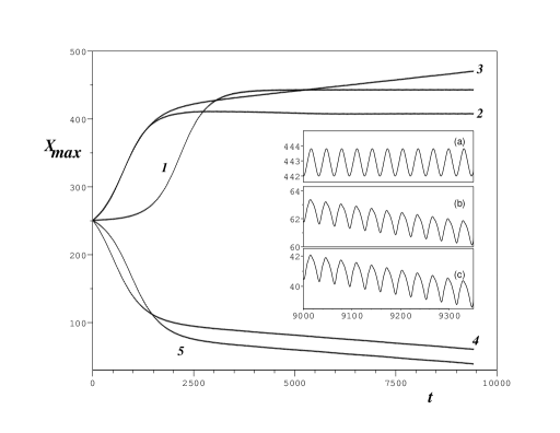
Figure 1: Time evolution of the kink center $X_{max}$ under action of the external magnetic field (10) for $J_{x}=0.2$, $J_{y}=0.5$, $J_{z}=1$, $\lambda=0.01$, $\omega=0.2$. Curve 1 corresponds to the case of single harmonic drive ($H_{1}=0.1$, $H_{2}=0$), curve 2 corresponds to $H_{1}=H_{2}=0.1$, $m=3$, $\theta=-2$. Curves 3-5 correspond to $H_{1}=H_{2}=0.1$, $m=2$, $\theta=-1$ (curve 3), $\theta=2.5$ (curves 4,5). The last two curves show evolution for different initial times: $t_{0}=T/4$ (curve 4) and $t_{0}=0$ (curve 5). Insets (a)-(c) give details of curves 1,4, and 5, respectively.

Curve 1 in this figure corresponds to the case of the single harmonic drive ($H_{2}=0$), where no directed DW motion is seen. Next, no directed DW motion is observed in the case of mixing two odd harmonics ($m=3$) as shown by curve 2. Curves 3-5 illustrate the evolution of the DW center for the case of two mixed harmonics with $m=2$. It is easy to notice that on the time scale $t>\lambda^{-1}$, the system settles on a periodic attractor (the periodicity can be observed from the insets in Figure 1) that corresponds to the motion in the direction, defined by the phase shift $\theta$. The simulations have been performed for different initial values of $\phi$ and initial times $t_{0}$, and in all the cases the system settles on the same attractor (compare, for example, curves 4 and 5).

The dependence $\langle v\rangle(\theta)$ of the average DW velocity on the phase shift between the harmonics, $\theta$, is shown in Figure 2.

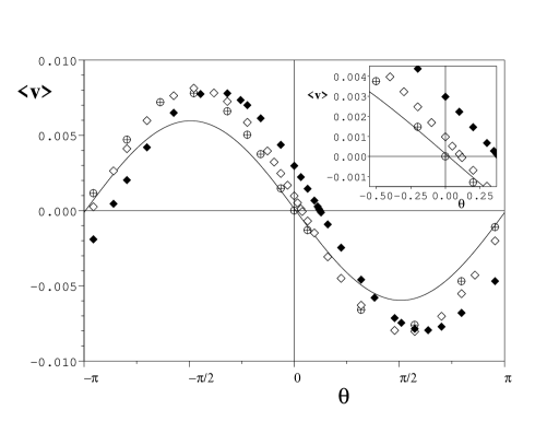
Figure 2: Dependence $\langle v\rangle=\langle v\rangle(\theta)$ for $\lambda=0.01$ ($\oplus$), $\lambda=0.1$ ($\diamond$, scaled by factor $1.3$), and $\lambda=0.3$ ($\blacklozenge$, scaled by factor $1.85$) computed numerically from equation (16). The perturbation theory result (15) for $\lambda=0.01$ is shown by solid line. Other parameters are chosen the same as for curves 3-5 in Figure 1. The inset shows details in the vicinity of $\theta=0$.

It appears to have a sinusoidal shape, as predicted by the perturbation theory result (15). Another demonstration of the validity of the symmetry approach is the behavior of the points where $\langle v\rangle(\theta)=0$. In Figure 2 along with the data for $\lambda=0.01$, the data for $\lambda=0.1$ and $\lambda=0.3$ have been plotted as well. Although these values of damping do not correspond to realistic values for magnets, these results are very instructive for the illustration of the restoration of the symmetries ${\widehat{\cal S}_{2\alpha}}$. Indeed, when $\lambda\to 0$, the values of $\theta$, at which the DW velocity becomes zero, gradually shift to $0,\pm\pi$. As shown already in Section 3, both the symmetries ${\widehat{\cal S}_{2\alpha}}$ are restored if $H_{z}(-t)=H_{z}(t)$. This happens if $\theta=0,\pm\pi$ [see equation (10)]. We would like also to point out good correspondence between the perturbation theory results (shown by the solid line) given by equation (15) and the results of direct integration of the LL equation.

Next, we consider the case of the magnetic field directed along the OX axis [${\bf H}(t)={\bf e}_{x}H(t)$], but which has the same functional dependence (10). According to the symmetry approach, this periodic drive does not yield the directed DW motion. The numerical simulations of this case are illustrated by Figure 3. The basins of attraction of two DW solutions that have opposite polarities and opposite velocities appear to be symmetric with respect to the value $\phi=0$. Indeed, if the initial value of the azimuthal angle is positive (see curves 1,3, and 5), the dynamics of the system settles on the attractor with the positive DW velocity ($v=0.00031$), while for negative values of $\phi$ (see curves 2,4 and 6) it tends to the solution with the DW velocity of opposite sign ($v=-0.00031$).

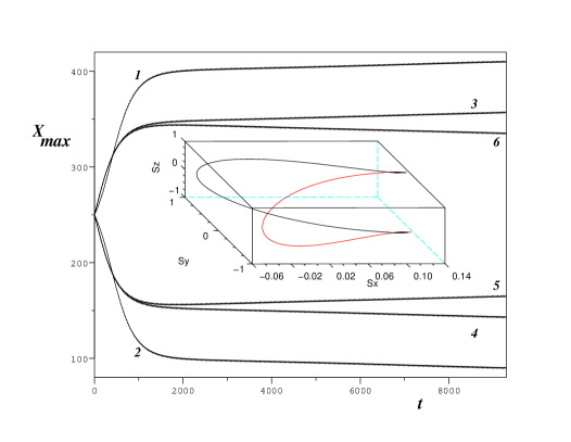
Figure 3: Time evolution of the kink center $X_{max}$ under action of the external magnetic field (10) for $H_{1}=H_{2}=0.05$, $\theta=1$, $m=2$ with initial azimuthal angle $\phi=\pi/10$ (curve 1), $\phi=-\pi/10$ (curve 2), $\phi=\pi/4$ (curve 3), $\phi=-\pi/4$ (curve 4), $\phi=3\pi/4$ (curve 5), and $\phi=-3\pi/4$ (curve 6). The rest of parameters is as in the case of Figure 1. The inset shows distribution of the magnetisation vector components $(S_{x},S_{y},S_{z})^{T}$ of DWs that correspond to curves 3 (black) and 4 (red) of the main figure.

In the case of ${\bf H}(t)||$OY, the same scenario is observed.

6 Discussion and conclusions

In this paper, the symmetry approach for the analysis of the unidirectional domain wall motion has been developed. The main objective was to demonstrate that a proper choice of the oscillating unbiased magnetic field can yield a net directed motion of the domain wall. With the help of the symmetry approach, we have obtained the necessary conditions to be imposed on the magnetic field in order to obtain the unidirectional motion. When the magnetic field is applied along a certain coordinate axis, this motion turns out to be possible only if this axis coincides with the easy axis, say OZ. The symmetry arguments prohibit the directed DW motion if the magnetic field is applied along any of the hard axes. The necessary condition for the directed DW motion in the presence of dissipation is given by $H_{z}(t)\neq-H_{z}(t+T/2)$. Next, we demonstrate the cubic dependence $\langle v\rangle\propto H_{1}^{2}H_{2}$ of the average DW velocity on the magnetic field amplitude. These results appear to be similar to those for topological solitons in the ac driven sine-Gordon (SG) equation sz02pre . Very recently, qca-n10pre a rigorous proof of the universality of these results for a wide range of nonlinear systems driven by the biharmonic signals of the type (10) has been obtained.

However there are certain differences in the directed soliton motion in the LL and SG cases. Due to the fact that the LL equation is three-component, while SG is scalar, there are more ways to apply the external field to the system, namely along any of three coordinate axes. But only in the case of magnetic field applied along the easy axis, the directed motion is possible. Here it should be stressed that we are interested in the average net motion which is independent from the the local properties of the DW such as handedness (polarity). The application of any ac signal along non-easy axes drives DWs with opposite polarities into opposite directions. The basins of respective attractors of the LL equation are symmetric with respect to the $\pi$-shift of the initial azimuthal angle. Therefore, a weak noise which is inevitable in realistic systems will lead to exploration of the whole phase space and eventually to zero net motion.

Another difference with respect to the SG case caused by the multicomponentness of the LL equation is a wider range of possibilities to drive a DW by external oscillating fields. Let us briefly discuss the case when two of the magnetic field components are nonzero. Consider first the case of magnetic field polarised in the easy plane XY [${\bf H}(t)=(H_{x}(t),H_{y}(t),0)^{T}$]: $H_{x}(t)=H_{0}^{(x)}\cos(m_{x}\omega t+\theta_{x})$, $H_{y}(t)=H_{0}^{(y)}\cos(m_{y}\omega t+\theta_{y})$. Here $m_{x},m_{y}=1,2,3,\ldots$, and they do not have a common divisor. Note that such a way to control the DW motion has been suggested in bgd90jetp for the particular case of $m_{x}=m_{y}=1$. The symmetry $\widehat{\cal S}_{1x}$ requires the simultaneous fulfilment of the equalities $H_{x}(t+T/2)=-H_{x}(t)$ and $H_{y}(t+T/2)=H_{y}(t)$. Similarly, the $\widehat{\cal S}_{1y}$ symmetry is present if both the equalities $H_{x}(t+T/2)=H_{x}(t)$ and $H_{y}(t+T/2)=-H_{y}(t)$ hold. If both $m_{x}$ and $m_{y}$ are odd, we have $H_{\alpha}(t+T/2)=-H_{\alpha}(t)\neq H_{\alpha}(t)$. Therefore none of the sets of equations (8) can be satisfied and thus both symmetries $\widehat{\cal S}_{1\alpha}$ are broken. If $m_{x}$ is even and $m_{y}$ is odd, we have $H_{x}(t+T/2)=H_{x}(t)\neq-H_{x}(t)$, thus $\widehat{\cal S}_{1x}$ is broken. But, $H_{y}(t+T/2)=-H_{y}(t)$, therefore $\widehat{\cal S}_{1y}$ is present. Similarly, if $m_{y}$ is even and $m_{x}$ is odd, the symmetry $\widehat{\cal S}_{1x}$ is satisfied and $\widehat{\cal S}_{1y}$ is broken. Therefore if one of $m_{x,y}$ is even and another one is odd, we expect no directed motion, whereas this motion must occur if both $m_{x,y}$ are odd.

Another way to drive unidirectionally a domain wall is to apply the oscillating magnetic field polarised in the plane that contains the easy axis k07pmm :
$H_{y}(t)=H_{0}^{(y)}\cos(m_{y}\omega t+\theta_{y})$, $H_{z}(t)=H_{0}^{(z)}\cos(m_{z}\omega t+\theta_{z})$; $m_{y},m_{z}=1,2,3,\ldots$. Alternatively, one can consider the field polarised in the XZ plane. If both $m_{y}$ and $m_{z}$ are odd, it is impossible to break simultaneously the set of equalities (8) and (9). In this case, the breaking of $\widehat{\cal S}_{1x}$ takes place because $H_{z}(t+T/2)=-H_{z}(t)$ but $H_{y}(t+T/2)=-H_{y}(t)\neq H_{y}(t)$. However, the symmetry $\widehat{\cal S}_{1y}$ is still present. If $m_{y}$ is even and $m_{z}$ is odd, we obtain $H_{z}(t+T/2)=-H_{z}(t)$ but $H_{y}(t+T/2)=H_{y}(t)\neq-H_{y}(t)$, therefore $\widehat{\cal S}_{1x}$ is present while $\widehat{\cal S}_{1y}$ is broken. If $m_{y}$ is odd and $m_{z}$ is even both the symmetries $\widehat{\cal S}_{1x,y}$ are broken because $H_{z}(t+T/2)=H_{z}(t)\neq-H_{z}(t)$. Therefore this is the only way to obtain the directed DW motion with the help of magnetic field polarised in the YZ plane.

Finally, we would like to outline the future directions of applications of the symmetry approach. It is of interest to consider topological magnetic excitations in two- and three-dimensional systems, where alongside the directed translational motion a unidirectional rotation can take place as well, as shown previously for particles dzfy08prl . Another question is how to apply the symmetry approach to the problem of DW directed motion in more complicated magnetic systems such as antiferromagnets, ferrites, magnetoelastic systems, and others. In this direction, some progress has already being accomplished in the papers ggg-d94prb ; gs95jmmm .

References

- (1) A.M. Kosevich, B.A. Ivanov, A.S. Kovalev, Phys. Rep. 194(3-4), 117 (1990)
- (2) H.J. Mikeska, M. Steiner, Adv. Phys. 40(3), 191 (1991)
- (3) F. Jülicher, A. Ajdari, J. Prost, Rev. Mod. Phys. 69, 1269 (1997)
- (4) P. Reimann, Phys. Rep. 361, 57 (2002)
- (5) P. Hänggi, F. Marchesoni, F. Nori, Ann. Phys. (Leipzig) 14(1-3), 51 (2005)
- (6) P. Hänggi, F. Marchesoni, Rev. Mod. Phys. 81, 387 (2009)
- (7) S. Flach, O. Yevtushenko, Y. Zolotaryuk, Phys. Rev. Lett. 84(11), 2358 (2000)
- (8) M.C. Marchesoni, Phys. Rev. Lett. 77(12), 2364 (1996)
- (9) M. Salerno, N.R. Quintero, Phys. Rev. E 65, 025602(R) (2002)
- (10) M. Salerno, Y. Zolotaryuk, Phys. Rev. E 65(5), 056603(10) (2002)
- (11) S. Flach, Y. Zolotaryuk, A.E. Miroshnichenko, M.V. Fistul, Phys. Rev. Lett. 88(18), 184101 (2002)
- (12) L. Morales-Molina, N.R. Quintero, A. Sánchez, F.G. Mertens, Chaos 16(1), 013117 (2006)
- (13) Y. Zolotaryuk, M. Salerno, Phys. Rev. E 73(6), 066621 (2006)
- (14) G. Carapella, G. Costabile, Phys. Rev. Lett. 87, 077002(4) (2001)
- (15) A.V. Ustinov et al, Phys. Rev. Lett. 93, 087001 (2004)
- (16) M. Beck et al, Phys. Rev. Lett., 95, 090603 (2005)
- (17) S. Flach, A.A. Ovchinnikov, Physica A 292, 268 (2001)
- (18) S. Savel’ev, A. Rakhmanov, F. Nori, New. J. Phys. 7 82 (2005).
- (19) S. Savel’ev, A.L. Rakhmanov, F. Nori, Phys. Rev. B 74 024404 (2006).
- (20) A. Himeno et al, J. Appl. Phys. 97 066101 (2005).
- (21) A. Alija et al, J. Phys. D: Appl. Phys. 42 045001 (2009).
- (22) E. Schlomann, J. Milne, IEEE Trans. Magn. 10, 791 (1974)
- (23) E. Schlomann, IEEE Trans. Magn. 11, 1051 (1975)
- (24) V. Bar’yakhtar, Y.I. Gorobyets, S. Denisov, Zh. Eksp. Teor. Fiz. (Sov. Phys. JETP) 98, 1345 (1990) [Sov. Phys. JETP 71, 751 (1991)]
- (25) P. Coullet, J. Lega, Y. Pomeau, Europhys. Lett. 15, 221 (1991)
- (26) G.E. Khodenkov, Phys. Met. Metallogr. 103(3), 228 (2007)
- (27) A. Aharoni, Introduction to the theory of ferromagnetism (Oxford University Press, Oxford, 2000)
- (28) E.K. Sklyanin, LOMI Preprint E-3-79 (1979)
- (29) L. Potemina, Sov. Phys. JETP 63, 562 (1986) [Sov. Phys. JETP 63, 562 (1986)]
- (30) Y.S. Kivshar, Physica D 40, 11 (1989)
- (31) N.R. Quintero, J.A. Cuesta, R. Alvarez-Nodarse, Phys. Rev. E 81(3), 030102 (2010)
- (32) S. Denisov, Y. Zolotaryuk, S. Flach, O. Yevtushenko, Phys. Rev. Lett. 100(22), 224102 (2008)
- (33) V.S. Gerasimchuk, Y.I. Gorobets, S. Goujon-Durand, Phys. Rev. B 49(14), 9608 (1994)
- (34) V. Gerasimchuk, A. Sukstanskii, J. Magn. Magn. Mater 146, 323 (1995)