Online Event Segmentation in Active Perception using Adaptive Strong Anticipation

Abstract

Most cognitive architectures rely on discrete representation, both in space (e.g., objects) and in time (e.g., events). However, a robot interaction with the world is inherently continuous, both in space and in time. The segmentation of the stream of perceptual inputs a robot receives into discrete and meaningful events poses as a challenge in bridging the gap between internal cognitive representations, and the external world. Event Segmentation Theory, recently proposed in the context of cognitive systems research, sustains that humans segment time into events based on matching perceptual input with predictions. In this work we propose a framework for online event segmentation, targeting robots endowed with active perception. Moreover, sensory processing systems have an intrinsic latency, resulting from many factors such as sampling rate, and computational processing, and which is seldom accounted for. This framework is founded on the theory of dynamical systems synchronization, where the system considered includes both the robot and the world coupled (strong anticipation). An adaption rule is used to perform simultaneous system identification and synchronization, and anticipating synchronization is employed to predict the short-term system evolution. This prediction allows for an appropriate control of the robot actuation. Event boundaries are detected once synchronization is lost (sudden increase of the prediction error). An experimental proof of concept of the proposed framework is presented, together with some preliminary results corroborating the approach.

1 Introduction

The perception of a robot is grounded on the physical world. Its sensors receive a continuous stream of information, as for instance the light patterns hitting the CCD sensor of a video camera. Cognitive representations, however, are often discrete, as in the case of events and objects. Although the usage of digital computers demand that all sensory information is discretized, this discretization is commonly performed in fixed, not always adjustable, discretization step (e.g, the frame rate and the pixel resolution of a video camera). The detection of meaningful events from a stream of sensory information is an important challenge, from the point of view of the design of a cognitive architecture for robots, contributing to bridge the gap between a continuous time world and discrete time, event-based cognitive representations.

The segmentation of a continuous stream of information into events is often overlooked, being commonly performed in an ad-hoc manner, either recurring to threshold values over heuristic functions, or fixed time triggers, for instance. But these methods are mostly sensor modality dependent, as well as task specific. This work addresses the problem of bridging the gap between the time continuous stream of sensory/actuation information, and the discrete time sequence of cognitive representations, proposing a modality and task independent framework for event segmentation.

This problem is addressed using a biologically inspired approach. Under this paradigm, our goal is not to faithfully model any aspect of the human brain, but rather to employ findings from neuroscience capable of providing guidance on how to engineer better systems.

The Event Segmentation Theory (EST) provides a model of how the human brain segments perception into a sequence of events [18, 7]. This model sustains that event segmentation is based on the detection of prediction errors in the sensory stream. Prediction is a commonplace mechanism found in many brain systems. In particular, the human brain is permanently making predictions and comparing them with the actual outcome [12]. Events are detected whenever a significant disparity between prediction and outcome is encountered. An event segmentation mechanism can be built following this principle, but the problem of how to make predictions about perceptions has to be addressed first.

Dubois distinguishes between strong and weak anticipation [3, 13]: the latter is based on an explicit model of the world, where the physics is encoded in analytical constructs, that can be mathematically solved given an initial condition. On the contrary, strong anticipation does not rely on a model, but rather on the dynamical evolution of the interaction of the agent with the world, seen as a single system. An example of strong anticipation can be found on the behavior of an outfield baseball player when catching a well-struck ball: weak anticipation of the ball landing position requires modeling the physics of the ball, encoding the initial state of the system (initial velocity, mass, friction coefficient, etc), and then predicting the landing position by solving the analytical model; in contrast, strong anticipation views the outfielder and the ball as a single system with new dynamics, as the outfielder moves itself driven by the projection of the ball on his retina. Empirical evidence suggest that this is the way an human outfield player functions [13]. In the context of robotics, a model based approach to anticipation may be appropriate for passive sensors, but when designing systems that actively engage in interactions with the world, as in the case of active perception, the world can no longer be modeled as an independent, self-contained system.

Stepp proposes an approach to strong anticipation based on the work developed in the field of chaotic systems concerning synchronization of dynamical systems [13]. Consider two systems, denoted D (drive) and R (response), connected by a unidirectional flow of information from D to R. It is possible to design the system R such that its dynamic evolution synchronizes with the one of D, regardless of the initial condition of each system. One way of doing this is for the R system to compare its state with the one of the D, and bias its dynamics accordingly, i.e., system R is controlled by a feedback loop, where the error results from this comparison. More interestingly, if this feedback loop contains a delay, system R is capable, under certain conditions, to anticipate system D [14]. Considering that system D includes both the robot and the world, and system R to be a model internal to the robot, this approach suggests an interesting mechanism to perform strong anticipation of the dynamical evolution of the world-robot system.

One problem remains to be solved: how to design system R? No system model is assumed a priori, since it depends on the coupling involving the robot and the world. A possible approach is to adapt system R during interaction. A solution to the adaptation of response systems in the context of dynamical systems synchronization has been proposed by Chen [1], where the convergence to the solution has been proved using the Lyapunov stability theory. This result does not directly apply, however, to anticipating synchronization.

The contributions of this work are:

• An event segmentation method based on Stepp’s strong anticipation concept [13], cast as an anticipating system synchronization framework;

• The application of Chen’s parameter identification method [1] to anticipating synchronization;

• A proof-of-concept implementation of an architecture for event segmentation and active perception, employing these methods.

This report is organized as follows: after a short section surveying related work, two sections on the theoretical background behind strong anticipation and the adaptation method to learn the response system R follow. Then, the proposed architecture for event segmentation is described, followed by some experimental results of a proof of concept implementation of these ideas. A section presenting some conclusions and open questions closes the report.

2 Related work

The problem of event segmentation has been studied in the past. See [10] for a review of recent techniques for the formation of event memories in robots. Ramoni et al. proposed a method to cluster robot activities using Markov chain models [11]. In [4] a batch maximum likelihood estimator is used to fit a sequence of time-indexed models to raw data. The incremental version of this algorithm is based on thresholding the likelihood of the current model along time. The spatio-temporal segmentation of video have been researched in [16], applying motion model clustering, and in [2] using hierarchical clustering of the 3D space-time video stream. Gesture segmentation and recognition has been addressed in [6] employing hidden-Markov models (HMM).

3 Strong anticipation

In [13] strong anticipation is modeled using a dynamical system synchronization framework. Consider two continuous dynamical state vectors $x(t),y(t)\in\mathbb{R}^{n}$ with the following coupled dynamics:

$$\begin{split}\dot{x}&=f(x)\\ \dot{y}&=f(y)+k(x-y_{\tau})\end{split}$$ (1)

where $y_{\tau}=y(t-\tau)$, i.e., a feedback loop with a constant delay $\tau$, and $k$ is a scalar gain. The first system is called the drive (D) while the second the response (R). This delayed feedback loop in the response system is a fundamental aspect, and is responsible for the response system capability of anticipating the trajectory of the drive.

This delayed feedback loop is neurophysiologically supported by the discovery of forward models in the brain, which predict sensory consequences of motor commands [8, 17, 5]. These models receive as input a copy of the subject motor action, and produce a prediction of future perceptions. For instance, when performing an arm movement, these models predict the trajectory followed by the arm, as perceived by the subject. One important function of this mechanism is to overcome the sensory processing latency in the brain, when the subject is performing controlled, quick movements.

To understand how the response system can anticipate the drive, consider that $\tau=0$ and that the systems are synchronized at time $t_{0}$, i.e., $x(t_{0})=y(t_{0})$. Under these conditions, the systems will remain synchronized, since $x-y_{\tau}=0$ and thus there is null feedback in the response. In this case, the concatenated state $z=(x,y)\in\mathbb{R}^{2n}$ evolves in the $x=y$ hyperplane, called the synchronization manifold [9]. The response system synchronizes with the drive if the error system with state $e=y-x$, also called the transversal system

$$\dot{e}=f(y)-f(x)-k\,e$$ (2)

is able to reject the perturbation $e$, driving it to zero. For $f(y)\simeq f(x)$, system (2) behaves like a first-order system with an exponential decay to zero. Anticipation is realized once $\tau>0$, as synchronization implies $x(t)=y_{\tau}=y(t-\tau)$ and thus $y(t)=x(t+\tau)$, meaning that the response anticipates the driver. This is called anticipating synchronization [14], where $x=y_{\tau}$ defines the anticipatory manifold [15].

Successful synchronization from an arbitrary initial condition is not guaranteed in general (unless for simple cases), and strongly depends on the values of $k$ and $\tau$. However, for any delay value $\tau$, $e(t)=0$ is a fixed point of the transversal system (2), meaning that once synchronized, the system will remain so. Voss conjectures that, if $e(t)=0$ is a stable fixed point for $\tau=0$, then there is a $\tau_{0}>0$ such that, for any $0<\tau<\tau_{0}$, the transversal system has a stable fixed point at $e(t)=0$. This conjecture has been backed up by numerical simulations [15].

In general, for sufficiently small $\tau$, stability of the transversal system can be expected. In the case of this work, since $\tau$ models the delay of the perceptual system (e.g., the latency from a change in the environment up to its detection by the computer vision algorithm), this delay can be assumed smaller than the time scale of the events being perceived.

4 Adaptive synchronization

In the previous section it was assumed that the dynamics of the drive and response systems are equal. If the drive system corresponds to the world-robot coupled system, its dynamics is not known a priori. One way of tackling this problem is to adapt the response system, online, during synchronization.

Chen proposes in [1] an approach to adapt response systems in the context of dynamical system synchronization. It does not account, however, for a delayed feedback.

Consider that the drive system has the form

$$\dot{x}=f(x)+F(x)\theta$$ (3)

where $\theta\in\mathbb{R}^{m}$ is a vector of (constant) parameters, $f(x)\in\mathbb{R}^{n}$ and $F(x)\in\mathbb{R}^{n\times m}$. The response system is identical, except for the parameter vector that is unknown, and for the synchronization feedback loop

$$\dot{y}=f(y)+F(y)\alpha+U(y,x,t,\alpha)$$ (4)

where $\alpha$ is the response parameter vector, and $U(y,x,t,\alpha)$ is called the controller of the response. Chen et al. proved in [1] that, under certain conditions, not only the response system synchronizes with the drive, but also that the response parameters $\alpha$ converge to the ones of the drive $\theta$, i.e.,

$$\lim_{t\rightarrow+\infty}||\alpha(t)-\theta||=0.$$ (5)

These conditions consist of the existence of a smooth controller $U(y,x,t,\theta)$ and of a scalar (Lyapunov) function $V(e)$, where $e=y-x$, such that:

1. $c_{1}||e||^{2}\leq V(e)\leq c_{2}||e||^{2}$,

2. the derivative of $V(e)$ along the solution of the coupled system

   $$\begin{split}\dot{x}&=f(x)+F(x)\theta\\ \dot{y}&=f(y)+F(y)\theta+U(x,y,t,\theta)\end{split}$$ (6)

   satisfies $\dot{V}(e)\leq-W(e)$, and

3. the parameter vector $\alpha$ is adapted according to the learning rule

   $$\dot{\alpha}(t)=-F^{T}(x)\left[\nabla V(e)\right]^{T}$$ (7)

   for $\nabla V(e)$ denoting the gradient (row) vector of $V$ with respect to $e$,

where $c_{1}$ and $c_{2}$ are two positive constants, $W(e)$ is a positive definite function, and $U(y,y,t,\theta)=0$.

This result has two important consequences: first, it proves convergence, provided that the response system is capable of synchronizing with the driver if $\alpha=\theta$ (i.e., if the true parameters were known), and second, it provides a learning law, in the form of the gradient of $\alpha$. However, in order to use this result, one has to find a controller $U$ and a function $V$ satisfying the premises of the theorem. Chen shows that the controller

$$U(y,x,t,\theta)=-e+f(x)-f(y)+\left[F(x)-F(y)\right]\theta$$ (8)

and the Lyapunov function

$$V(e)=\frac{1}{2}e^{T}e$$ (9)

satisfy the premises for any $F$ and $f$.

The practical application of these results raises three practical issues. One is the assumption that functions $F$ and $f$ are known, meaning that one should have a prior knowledge of the structure of the dynamics of the system. One can reverse this argument, stating that, given functions $f$ and $F$ sufficiently generic, this method allows the adaptation to any dynamical system that can be modeled by (3) for some parameter vector $\theta$. Second, this result was proved for continuous time systems. The discretization of $\dot{\alpha}$ raises the issue of the choice of a learning rate (hidden in a proportionality constant of $V$, since the theorem is invariant to a change of scale of this Lyapunov function). Finally, the third issue concerns hidden state variables: if there is a state variable that is hidden, i.e., the Lyapunov function $V(e)$ does not depend on its error, then this function is no longer positive definite. This requires that all drive state variables have to be fed to the response system controller. This is mostly true once the state variables considered are all obtained from perception (as in the case of the outfield baseball player example above).

5 Event segmentation

The event segmentation framework we propose in this work, depicted in Figure 1, consists of a pair of response systems, one performing adaptation (labeled adaptive response), and the other anticipation (labeled anticipating response). The adaptive response learns the parameter vector $\alpha$ as described in the Adaptive synchronization section, while anticipating response performs anticipating synchronization as explained in the Strong anticipation section. The robot-world coupled system is modeled by the controlled drive system. Note that the access of the architecture to the world state is subject to a delay, modeling for instance the latency of the perceptual channel (image acquisition, processing, and tracking). The controller computes the actuation vector $u$ based on the anticipated world state $y$.

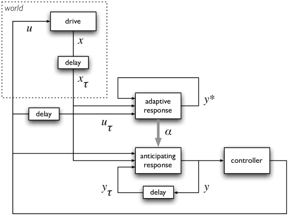
Figure 1: System architecture, consisting of the drive system and the perceptual delay (world), and the double response system formed by the adaptive and the anticipating responses. The anticipating response uses the parameters $\alpha$ obtained by the adaptive response. The control input $u$ is obtained by a controller fed with the anticipated state $y$.

The drive system, together with the perceptual delay, is modeled by the dynamical system

$$\dot{x}=f(x)+F(x)\theta+u$$ (10)

where $u$ is the control input, modeling the actuation of the robot in the world. Shifting this equation by a delay of $\tau$ one obtains

$$\dot{x}_{\tau}=f(x_{\tau})+F(x_{\tau})\theta+u_{\tau}$$ (11)

where $u_{\tau}(t)=u(t-\tau)$. This model can be put in the form of (3) defining a time varying function

$$f_{\tau}(x_{\tau},t)=f(x_{\tau})+u_{\tau}$$ (12)

from which $\dot{x}_{\tau}=f_{\tau}(x_{\tau},t)+F(x_{\tau})\theta$. The adaptive response receives the delayed state $x_{\tau}$, together with the delayed control input $u_{\tau}$

$$\dot{y}^{*}=f(y^{*})+F(y^{*})\alpha+u_{\tau}+U(y^{*},x_{\tau},t,\alpha)$$ (13)

Once $f_{\tau}(y^{*},t)=f(y^{*})+u_{\tau}$, this equation can be put in the form of (4). The anticipating response is described by

$$\dot{y}=f(y)+F(y)\alpha+u+k(y_{\tau}-x_{\tau})$$ (14)

where $y_{\tau}=y(t-\tau)$ as before, and the parameter vector $\alpha$ equals the one obtained by the adaptive response. The anticipatory synchronization manifold is defined by $y_{\tau}=x_{\tau}$. Thus, $y=x$, meaning that the anticipating response is synchronized with the drive system, which is the same to say that it is anticipating the delayed perception $x_{\tau}$. By shifting (12) in time one can get $f_{\tau}(y,t+\tau)=f(y)+u$, allowing us to write (11) and (14) as

$$\begin{split}\dot{x}_{\tau}&=f_{\tau}(x_{\tau},t)+F(x_{\tau})\theta\\ \dot{y}&=f_{\tau}(y,t+\tau)+F(y)\alpha+k(y_{\tau}-x_{\tau})\\ \end{split}$$ (15)

thus matching (1) (except for the time varying dynamics, which do not affect the previous considerations on anticipating synchronization) when $\alpha=\theta$.

According to the theory of Event Segmentation  [18], perceptual systems continuously make predictions about perceptual input, and perceive event boundaries when transient errors in prediction arise. On the adaptive synchronization framework, the Lyapunov function $V(e)$ defined in (9), for $e=y^{*}-x_{\tau}$ provides a solid estimate of the prediction error. Considering the function values in a time window, we can associate the obtained samples with a random variable with Normal distribution of mean $\mu_{V}$ and variance $\sigma^{2}_{V}$. Under this assumption, the normalized metric

$$b_{V}=\frac{V-\mu_{V}}{\sigma_{V}}$$ (16)

is normally distributed with zero mean and unit variance. When $|b_{V}|$ exceeds a threshold $b_{\textrm{event}}$, an event boundary is detected. If $b_{V}$ is normally distributed with zero mean and unit variance, the cumulative probability of the distribution tails for $|b_{V}|>b_{\textrm{event}}$ is the probability of false positive detection. Thus, $b_{\textrm{event}}$ should be sufficiently high so that false positive detection is minimized, but low enough in order to detect the prediction error increase due to a sudden change in the dynamics of the system.

6 Experimental results

As a proof of concept for the ideas presented here, a simple scenario was simulated: a ball rolling free on a series of inclined planes, with different slopes, is observed by a robot camera which aims to follow it, in order to center it on the image, as depicted in Figure 2. The camera moves parallel to the plane, for simplicity sake.

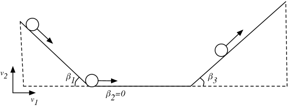
Figure 2: Simulated scenario, where $\beta_{1}=\beta_{3}=\pi/12$.

Denoting the ball coordinates by $v=[v_{1}\>v_{2}]^{T}$ and the camera coordinates by $c=[c_{1}\>c_{2}]^{T}$, the ball projection $x=[x_{1}\>x_{2}]^{T}$ in the image plane is assumed orthographic: $x=v-c$. Assuming that there is no ground friction, the dynamics of the ball is a double integrator

$$\begin{split}\ddot{v}_{1}&=-g\sin\beta\cos\beta\\ \ddot{v}_{2}&=-g\sin^{2}\beta\\ \end{split}$$ (17)

Considering that the camera support is frictionless and that its movement is controlled in acceleration (i.e., force control), the resulting drive system, in state space form, is given by

$$\begin{split}\ddot{x}_{1}&=-g\sin\beta\cos\beta-\ddot{c}_{1}\\ \ddot{x}_{2}&=-g\sin^{2}\beta-\ddot{c}_{2}\\ \dot{x}_{1}&=\dot{x}_{1}\\ \dot{x}_{2}&=\dot{x}_{2}\\ \end{split}$$ (18)

considering the state vector $x=[\dot{x}_{1}\>\dot{x}_{2}\>x_{1}\>x_{2}]^{T}$. This system can be put in the form (10) once

$$\begin{split}f(x)&=\left[\begin{array}[]{c}0\\ 0\\ \dot{x}_{1}\\ \dot{x_{2}}\end{array}\right]\\ \theta&=\left[\begin{array}[]{c}-g\sin\beta\cos\beta\\ -g\sin^{2}\beta\\ \end{array}\right]\end{split}\quad\begin{split}F(x)&=\left[\begin{array}[]{cc}1&0\\ 0&1\\ 0&0\\ 0&0\\ \end{array}\right]\\ u&=\left[\begin{array}[]{c}-\ddot{c}_{1}\\ -\ddot{c}_{2}\\ 0\\ 0\end{array}\right]\end{split}$$ (19)

For this proof of concept, we set the response system to be structurally identical, thus employing the same functions $f$ and $F$, and control input $u$. The vector $\alpha=[\alpha_{1}\>\alpha_{2}]^{T}$ is the parameter vector to be adapted according to Chen’s learning rule (7).

When the anticipating response is synchronized with the drive, we have $x=y$, and thus the dynamics of the anticipating response becomes

$$\ddot{y}=\alpha-\ddot{c}.$$ (20)

The camera motion controller considered has the form

$$\ddot{c}=k_{p}y+k_{d}\dot{y}+\alpha$$ (21)

where $k_{p}$ and $k_{d}$ are the proportional and the derivative gains of the controller. Thus, the closed loop dynamics becomes

$$\ddot{y}=-k_{p}y-k_{d}\dot{y}$$ (22)

The design of the controller gains $k_{p}$ and $k_{d}$ can be performed by pole placement (in the experiments we set $k_{d}^{2}=4k_{p}$, yielding a smooth response with a double pole at $-k_{d}/2$).

The experiments were conducted after discretizing the above equations using a simple approximation $\dot{z}(t)\simeq[z(t+T)-z(t)]/T$. The sampling rate was 100Hz, $k_{p}=1$, $k_{d}=2$, $k=1$, and the Lyapunov function used was (9). The delay considered was $\tau=0.65s$ (65 samples). Event boundaries are detected using a 10-second window and a $b_{\mathrm{event}}=3$. The system is initialized with the ball starting on the top left position of the ramp, and as the ball transverses the scenario there are two events, corresponding to the two changes of the ramp slope. Each simulation takes 100s of simulated time.

Figure 3 attests the performance of the adaptive response system, in terms of the evolution of the parameters $\alpha$, compared with the ground truth ($\theta$, that changes with the slope). As can be seen, the parameter vector $\alpha$ converges to the true parameters $\theta$ after some time.

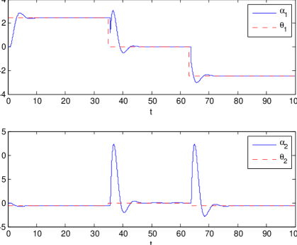
Figure 3: Parameters $\alpha$ evolution (solid line) in comparison with the true values (dashed line).

Figure 4 shows the evolution of the ball position in the camera without an anticipating response system, i.e., the camera motion controller is fed by $y^{*}$ instead of $y$. As expected, the delay introduced by the latency of the perceptual channel jeopardizes the control of the camera. Also, the adaptive response follows the drive with a delay of $\tau$.

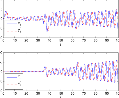
Figure 4: System response without anticipation.

Figure 5 compares the ball position in the camera with its anticipated response. In this case, both are synchronized, since the ball coordinates in the image converge to zero (except for a brief time after each slope change, while the adaptive system learns the new parameters). Also, the anticipating response makes it possible to control the drive system satisfactorily.

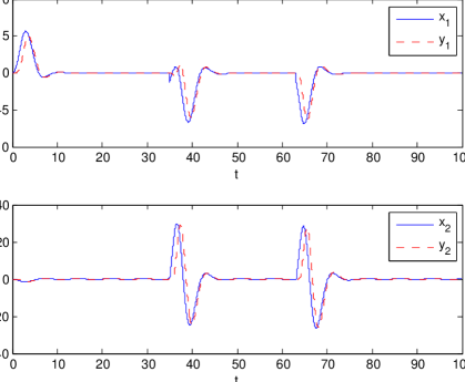
Figure 5: System response using the full architecture.

Figure 6 pictures the evolution of the prediction error estimate $V(e)$. Its value approaches zero as the drive and response system become synchronized.

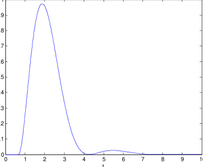
Figure 6: Prediction error $V$ for the first 10 seconds of the simulation.

Finally, Figure 7 shows the event segmentation results obtained using the normalized metric (16), with a window of 10s. As expected, each change of plane is detected as an event boundary by the framework. Interestingly, the peak of this metric, at the event boundary, increases with the window size, without any loss of temporal resolution.

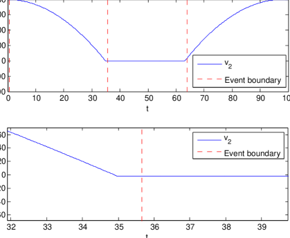
Figure 7: The ball $v_{2}$ coordinate evolution along the experiment: top plot shows the detected events, and the bottom plot a zoom around the first detected event. The delay observed in this second plot corresponds to the perceptual delay $\tau$.

These results show that the proposed system is capable of correctly (1) detecting the event boundaries that correspond to the change of ramp slope by the ball, (2) controlling the camera movement using anticipation, and (3) learning the correct system parameters.

7 Conclusions and future work

This report describes an event segmentation framework, targeting active perception in robots, based on the concept of strong anticipation proposed by Stepp et al. in [13]. A dynamical system synchronization paradigm is used as theoretical foundation of the proposed architecture, where the robot-world coupled system is identified using a parametric method for adaptation proposed by Chen et al. in [1], and the actuation is performed using anticipation. This anticipation accommodates for the net delay of the perceptual channel. The capability of the architecture to anticipate perception allows the robot to control its actuation based on the prediction of the robot-world state, instead of relying on the delayed perceptual data.

Having the described proof of concept experiments shown that the proposed architecture behaves as expected, future work includes scaling this approach to more complex domains. This involves tackling the issues of the learning rate, which is hidden in the proportionality constant of the Lyapunov function, used in the Chen’s learning rule, as well as the automatic design of the controller, given the adapted parameters. Other open questions include dealing with hidden state variables, as well as complex relations among objects (e.g., grasping, occlusion, and so on).

References

- [1] Shihua Chen and Jinhu Lü. Parameters identification and synchronization of chaotic systems based upon adaptive control. Physics Letters A, 299:353–358, 2002.
- [2] D. DeMenthon. Spatio-temporal segmentation of video by hierarchical mean shift analysis. Language, 2, 2002.
- [3] Daniel M. Dubois. Mathematical foundations of discrete and functional systems with strong and weak anticipations. In Anticipatory Behavior in Adaptive Learning Systems, Lecture Notes in Computer Science, pages 107–125. Springer, 2003.
- [4] V. Guralnik and J. Srivastava. Event detection from time series data. In Proceedings of the fifth ACM SIGKDD international conference on Knowledge discovery and data mining, pages 33–42. ACM, 1999.
- [5] Mitsuo Kawato. Internal models for motor control and trajectory planning. Current Opinion in Neurobiology, 9(6):718–727, December 1999.
- [6] Daehwan Kim, Jinyoung Song, and Daijin Kim. Simultaneous gesture segmentation and recognition based on forward spotting accumulative hmms. Pattern Recognition, 40(11):3012–3026, November 2007.
- [7] Christopher A. Kurby and Jeffrey M. Zacks. Segmentation in the perception and memory of events. Trends in Cognitive Sciences, 12(2):72–79, February 2008.
- [8] R.C. Miall, D. J. Weir, D. M. Wolpert, and J. F. Stein. Is the cerebellum a smith predictor? Journal of Motor Behavior, 25(3):203–216, 1993.
- [9] Louis M. Pecora, Thomas L. Carroll, Gregg A. Johnson, and Douglas J. Mar. Fundamentals of synchronization in chaotic systems, concepts, and applications. Chaos, 7(4):520–543, 1997.
- [10] Erich Prem, Erik Hörtnagl, and Georg Dorffner. Growing event memories for autonomous robots. In Proceedings of the Workshop On Growing Artifacts that Live: Basic Principles and Future Trends, 2002.
- [11] Marco Ramoni, Paola Sebastiani, and Paul Cohen. Unsupervised clustering of robot activities: a bayesian approach. In Proceedings of the fourth international conference on Autonomous agents (AGENTS’00), pages 134–135, 2000.
- [12] Wolfram Schultz and Anthony Dickinson. Neuronal coding of prediction errors. Annual Review of Neuroscience, 23:473–500, 2000.
- [13] N. Stepp and M.T. Turvey. On strong anticipation. Cognitive Systems Research, 11:148–164, 2010.
- [14] Henning U. Voss. Anticipating chaotic synchronization. Physical review E, 61(5):5115–5119, 2000.
- [15] Henning U. Voss. Dynamic long-term anticipation of chaotic states. Physical Review Letters, 87(1):14102, July 2001.
- [16] J.Y.A. Wang and E.H. Adelson. Spatio-temporal segmentation of video data. In SPIE Proceedings Image and Video Processing II, volume 2182, pages 120–131, 1994.
- [17] Daniel M. Wolpert, R. Chris Miallb, and Mitsuo Kawato. Internal models in the cerebellum. Trends in Cognitive Sciences, 2(9):338–347, 1998.
- [18] Jeffrey M. Zacks, Nicole K. Speer, Khena M. Swallow, Todd S. Braver, and Jeremy R. Reynolds. Event perception: A mind–brain perspective. Psychological Bulletin, 133(2):273–293, 2007.