Observational Constraints for $\delta\mu$ Mixing

Abstract

We provide a brief review of thermohaline physics and why it is a candidate extra mixing mechanism during the red giant branch (RGB). We discuss how thermohaline mixing (also called $\delta\mu$ mixing) during the RGB due to ${}^{3}\mathrm{He}$ burning, is more complicated than the operation of thermohaline mixing in other stellar contexts (such as following accretion from a binary companion). We try to use observations of carbon depletion in globular clusters to help constrain the formalism and the diffusion coefficient or mixing velocity that should be used in stellar models. We are able to match the spread of carbon depletion for metal poor field giants but are unable to do so for cluster giants, which may show evidence of mixing prior to even the first dredge-up event.

1 Introduction

The need for extra mixing on the RGB is observationally well established. Any mechanism (or the combined effect of multiple mechanisms) must meet the following requirements:

1. It must occur after the luminosity bump and continue to operate until near the tip of the RGB. (Gilroy & Brown, 1991; Weiss & Charbonnel, 2004; Smith & Martell, 2003; Martell et al., 2008)

2. It must occur over a range of masses and metallicities. (Smiljanic et al., 2009)

3. It must deplete ${}^{7}\mathrm{Li}$. (Charbonnel et al., 1998; Smiljanic et al., 2009)

4. It must deplete ${}^{3}\mathrm{He}$. (Dearborn et al., 1986; Hata et al., 1995; Dearborn et al., 1996)

5. It must lower the ${}^{12}\mathrm{C}$/${}^{13}\mathrm{C}$ ratio (Charbonnel, 1994, 1996)

6. It must deplete the carbon abundance and increase the nitrogen abundance. (Smiljanic et al., 2009; Smith & Martell, 2003; Martell et al., 2008)

These criteria suggest that, in order for theory to remain consistent with observations, material must be mixed through radiative regions, processed by the H-shell, and mixed back into the enevelope. This requirement is often referred to as deep mixing because mixing deeper than the formal convective boundary into the radiative zones will lead to material being exposed to regions of higher temperature and will result in the required additional processing. In general the ${}^{12}\mathrm{C}$/${}^{13}\mathrm{C}$ ratio is used to probe the efficiency of first dredge up (FDU); (Dearborn et al., 1975; Tomkin et al., 1976) and is also used as a tracer of the extent of deep mixing. A good example of this was Sweigart & Mengel (1979) who were the first to use the isotopes to investigate the role of rotational mixing on the RGB. More recently Palacios et al. (2006) have shown that, whilst rotation does reduce the ${}^{12}\mathrm{C}$/${}^{13}\mathrm{C}$ isotopic ratio, it is unable to explain the values seen in giant photospheres. Although it is understood that extra mixing must take place, only recently has a mechanism (i.e. thermohaline mixing) been discovered that can potentially satisfy all of the aforementioned criteria (Eggleton et al., 2006).

2 Thermohaline Mixing In Stars

2.1 Historical Overview

Thermohaline mixing was first studied in the Earth’s oceans by Stern (1960) where stratified warm salty water sits upon a cool unsalted layer. The layers are initially stable. However, heat diffuses more quickly than composition so the warmer layers cool. Now they are simply denser than the material underneath, and a turnover is initiated via the formation of lengthy “fingers” of cooler salty water reaching down into the cold fresh water. This displaces cool fresh water upwards, and a mixing occurs. On a slower timescale the salt diffuses out of the salty cool water to reach a new saltiness in the mixed region.

This double diffusive mixing was first applied to a stellar context by Stothers & Simon (1969). Ulrich (1972) applied this to a perfect gas and Kippenhahn et al. (1980) extended this to allow for a non-perfect gas which included radiation pressure and degeneracy. There were two obvious situations in which they applied thermohaline mixing. Firstly, during pre-main sequence contraction when in-situ ${}^{3}\mathrm{He}$ burning lowers the local mean molecular weight, $\mu$ because the reaction

$$^{3}\mathrm{He}\left({}^{3}\mathrm{He},2\rm{p}\right)^{4}\mathrm{He}$$ (1)

produces more particles than it destroys. The mixing is determined by the competition of the heat diffusion and the difference in composition but it is driven by the change in local molecular weight. This was found to have little effect, due to the short pre-main-sequence time scale and the fact the star becomes fully convective before reaching the Zero Age Main Sequence (ZAMS). The second case consisdered was during the core flash, when during off-centre He ignition, carbon-rich material sits upon helium-rich material. This also was considered to have little effect on the evolution primarly due to the uncertainty of competing timescales. The mixing must occur before the star settles down to quiescent helium burning. Eggleton et al. (2006) also showed that a small amount of overhooting inwards could remove the molecular weight inversion on a dynamical timescale.

2.2 Application to the RGB

Eggleton et al. (2006) used a 3D hydrodynamical stellar code (Dearborn et al., 2006) to show an instability develops due to ${}^{3}\mathrm{He}$ burning along the RGB, an instability that Charbonnel & Zahn (2007) model as thermohaline mixing. Charbonnel & Zahn (2007) and Eggleton et al. (2008) have modelled this ${}^{3}\mathrm{He}$ burning driven instability in their 1D codes and demonstrated the significant effect the mixing has during the RGB. Following FDU, the convective envelope recedes, leaving behind a homogeneous region. Any composition and molecular weight gradient has been removed due to the convective mixing. As the hydrogen burning shell begins to advance, ${}^{3}\mathrm{He}$ begins to burn. From Equation 1 it can be seen that this reaction creates a local molecular weight inversion; Eggleton et al. (2008) found its magnitude to be of the order ${\bigtriangleup\mu}/{\mu}$ $\sim$ 10^-4. Although the inversion seems small, convection is in fact driven by a similarly small superadiabaticity. Usually such a small change in the local molecular weight would have almost no effect, as it would be swamped by the existing $\mu$ gradient produced by the burning of other species. It is this unique situation where ${}^{3}\mathrm{He}$ begins to burn before the other species and the fact that first dredge up has homogenised the region that allows the inversion to develop.
Although there is no salt in the star the process is doubly diffusive and thus labelled thermohaline mixing. The authors refer to this as $\delta\mu$ mixing to emphasise that the mechanism that drives the mixing and the fact it is more complex than the other examples of thermohaline mixing. As ${}^{3}\mathrm{He}$ burns, a parcel forms that is hotter and has lower molecular weight than its surroundings. It quickly expands (and begins to cool) in order to establish pressure equilibrium. The expansion reduces the density and therefore the element becomes buoyant. The parcel rises until it finds an equilibrium point where the external pressure and density are equal to that inside the bubble. This is expected to be a small displacement which occurs on a dynamical timescale.

As the molecular weight inside the bubble is lower than its surroundings the equilibrium point must correspond to a place where the external temperature is higher than that of the bubble. The temperature inside the bubble will be lower than its surroundings:

$$\rm{\frac{T_{i}}{T_{o}}=\frac{\mu_{i}}{\mu_{o}}},$$ (2)

where subscript i denotes the inside of the bubble and subscript o denotes the surroundings. As heat begins to diffuse into the parcel, we expect layers will start to strip off in the form of long fingers. It is this secondary mixing that governs the overall mixing timescale. The mixing cycles in fresh ${}^{3}\mathrm{He}$ from the envelope reservoir, while CN-processed material is cycled into the convection zone.
Eggleton et al. (2008, EDL hereafter) found that this mixing satisfies the criteria outlined in Section 1. The level of depletion of the carbon isotopes will depend on the efficiency of the mechanism. EDL estimated the mixing speed and with their formula for the diffusion coefficient found that a window of three orders of magnitude in the mixing velocity can lead to observed levels of ${}^{12}\mathrm{C}$/${}^{13}\mathrm{C}$ and ${}^{3}\mathrm{He}$ depletion. Ulrich (1972) and Kippenhahn, Ruschenplatt, & Thomas (1980) use essentially the same formula for the diffusion coefficient (UKRT hereafter) but their geometric coefficients vary by two orders of magnitude. Charbonnel & Zahn (2007) have applied the UKRT mixing to the RGB. Both Charbonnel & Zahn (2007) and EDL see the ${}^{12}\mathrm{C}$/${}^{13}\mathrm{C}$ ratio is reduced to similar levels. In this study we will attempt to use globular cluster observations to constrain both the form of the diffusion coefficient and the mixing velocity.

3 The Mixing Speed

In order to implement $\delta\mu$ mixing into our 1D codes we must consider the following:

1. Which formalism should be used? Here we will limit our investigation to the EDL and UKRT prescriptions for the diffusion coefficient.

2. Once the preferred formalism is identified what mixing velocity is needed to match observations? What values do we use for any free parameters?

3. The ${}^{12}\mathrm{C}$/${}^{13}\mathrm{C}$ ratio is generally used as a proxy to probe the extent of mixing. This quickly saturates in low metallicity stars and therefore could be misleading. Is there a better way to try to constrain the velocity?

EDL postulated the following formula based on the velocities from their 3D code in analogy with the existing convective formalism in their code:

$$D=\left\{\begin{array}[]{ccc}\frac{{F_{\rm inv}}r^{2}}{{t_{\rm nuclear}}}{\thinspace}(\mu-\mu_{\rm min})&\mbox{ if }(k\geq k_{\rm min})\\ \\ 0&\mbox{ if }(k\leq k_{\rm min}),\end{array}\right.$$ (3)

where $\mu_{\rm{min}}$ is the smallest value of $\mu$ in the current model, $k$ the mesh point number, counted outwards from the centre, $r$ is the radial coordinate, $F_{\rm{inv}}$ is a constant which is selected to obtain the desired mixing efficiency and ${t_{\rm nuclear}}$ is an estimate of the nuclear evolution timescale (see EDL).

This formulation ensured the correct region was mixed but ensures the mixing is formally zero at the position where $\mu$ has its minimum even though it should presumably be the most efficient at this point. EDL give upper and lower estimates for the mixing velocity and find that they can alter the speed by three orders of magnitude and still produce the observed levels of ${}^{12}\mathrm{C}$/${}^{13}\mathrm{C}$ and ${}^{3}\mathrm{He}$. Charbonnel & Zahn (2007) adopt the UKRT formula

$$D_{t}=C_{t}\,K\left({\varphi\over\delta}\right){-\nabla_{\mu}\over(\nabla_{\rm ad}-\nabla)}\quad\hbox{for}\;\nabla_{\mu}<0,$$ (4)

where $\nabla=(\partial\ln T/\partial\ln P)$, $\varphi=(\partial\ln\rho/\partial\ln\mu)_{P,T}$, $\delta=-(\partial\ln\rho/\partial\ln T)_{P,\mu}$ and $C_{t}$ is the geometric factor.

Empirical studies of fluids in laboratory conditions led Ulrich (1972) to determine that $C_{\rm{t}}$ $\sim$ 1000. He saw the development of long salt fingers with lengths that were larger than their diameters, which led to efficient mixing. Kippenhahn on the other hand envisaged the classical picture where mixing is due to blobs and thus determined $C_{\rm{t}}$ $\sim$ 10.

We have run stellar models of various masses, with both EDL and UKRT mixing. We tested different values of $F_{\rm{inv}}$ and $C_{\rm{t}}$ in order to alter the efficiency of mixing. To test our models for the extra mixing we chose to use the carbon abundance as a function of $M_{\rm{V}}$ as determined by Smith & Martell (2003). They plotted carbon abundance as a function of visual magnitude for a variety of globular clusters. In doing so they were able to clearly demonstrate the depletion of carbon along the RGB. Globular cluster have always been an excellent test bed for stellar theory and by trying to match the carbon depletion for various red giant branches we have an alternative abundance test for mixing efficiency.

4 Results

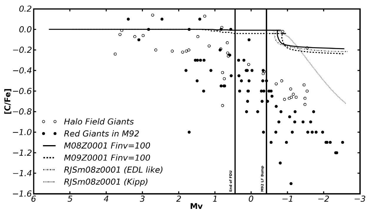
Figure 1: We plot the carbon abundance [C/Fe] as a function of $M_{\rm{V}}$ for observed giants and our models. We include cluster giants from M92 (solid circles) along with Galactic halo field giants (open circles) where the metallicity covers [Fe/H] =-1 to -2. Both sets of observational data were taken fromSmith & Martell (2003). The solid line and the bashed line correspond to models run with MONSTAR. The solid black line is the evolutionary track for a 0.8 $\rm{M}_{\odot}$ star up until the core flash. The dashed line is the evolution of a 0.9 $\rm{M}_{\odot}$ star. The dotted and dot-dashed lines are models run with the Eggleton code which has been modified by Stancliffe & Eldridge (2009). The dot-dashed line corresponds to the evolution of a 0.8 $\rm{M}_{\odot}$ star using an EDL formalism. The dotted line is for a 0.8 $\rm{M}_{\odot}$ star using a UKRT style mixing and $C_{\rm{t}}$ = 1000.

In Figure 1 we plot carbon abundance for stars in the Galactic globular cluster M92 and the Galactic halo from Smith & Martell (2003). Open circles denote galactic field giants whose metallicity ranges from -2.0 $\leq$ [Fe/H] $\leq$ -1.0 also taken from Smith & Martell (2003) . The filled circles correspond to RGB stars in M92. In both the field and the halo it is immediately obvious that there is carbon depletion as stars ascend the giant branch. If our models are able to match the carbon depletion we may be able to constrain the thermohaline mixing formalism and velocity. Another thing to notice before turning to the models is the spread in carbon for a given visual magnitude. We attribute this to the primordial abundances of the cluster with the most C-rich at a given magnitude being the “normal” stars. The spread in C at a given magnitude is assumed to be of primordial origin as is the case with many other globular clusters. Our primary aim is to match the level of carbon depletion. That is, we are concerned with matching the decrease in the upper and lower limits of the [C/Fe] values, as a function of magnitude. The solid and dashed lines were computed using MONSTAR (Campbell & Lattanzio 2008). We have evolved a 0.8 $\rm{M}_{\odot}$ and a 0.9 $\rm{M}_{\odot}$ star until the core flash. These masses straddle the age limits of stars in this cluster. A metallicity of Z=0.0001 was used to match that of the M92 where [Fe/H]=-2.2 (Bellman et al., 2001). The EDL mixing quickly destroys the ${}^{3}\mathrm{He}$ without significantly altering the FDU values of carbon. We believe this model is not mixing to high enough temperatures. As mentioned in the previous section, the mixing speed is formally zero at the position where $\mu$ has its minimum. By not mixing at the minimum properly the $\mu$ profile is being affected and carbon is not being exposed to the required temperature in either model.
The dot-dashed line is a model computed using the Eggleton code, (Eggleton, 1971; Stancliffe & Eldridge, 2009). It too is of mass 0.8 $\rm{M}_{\odot}$ and corresponds to the metallicity of M92 however it is run without mass loss. Running without mass loss here will result in less carbon depletion than we would otherwise expect, therefore will serve as a lower limit for the depletion of carbon. An EDL style formula for the diffusion coefficient is used in this calculation, that is there is a dependence on the position where $\mu$ reaches it’s minimum. The $F_{\rm{inv}}$ here was cailbrated such that a 1.5 $\rm{M}_{\odot}$, Z=0.0001 model gave the same level of carbon depletion on the RGB as a 1.5 $\rm{M}_{\odot}$ Z=0.0001 model with UKRT mixing where $C_{\rm{t}}$=1000, (see Stancliffe 2010 for more detail).

The dotted line is a model with a UKRT prescription taken from Stancliffe et al. (2009) where $C_{\rm{t}}$=1000. This also was run without mass loss. The UKRT mixing is a local formalism that is dependent on the $\mu$ gradient. Unlike in the EDL case this translates to the mixing being more efficient at the position where $\mu$ reaches its minimum. In both cases carbon is brought down from the envelope but here it is mixed to the position of lowest molecular weight and hence exposed to the shell much faster. The high temperature gradient ensures that mixing only a little deeper will see the carbon undergo larger depletion. This is of course all dependent on the amount of ${}^{3}\mathrm{He}$ available to drive the mixing. We see that the UKRT mixing can lead to levels of depletion seen in the field giants. Given that the field giants and M92 stars are of similar age and metallicity it is interesting the cluster stars undergo more substantial depletion. We defer the discussion of why this is to subsequent work.

5 Conclusion

Our initial motivation behind this paper was to use the observed variation of carbon abundances on the giant branch to help constrain some of the uncertainties present in the thermohaline mixing which we believe is operating during the red-giant phase. Drawn by the best data being available for M92, we chose this as our first attempt to fit the observations. The fact that we have failed in our aim has nevertheless taught us three important things:

1. The functional form of the diffusion co-efficient strongly influences the depletion of carbon.

2. Comparing the carbon isotope ratio is not necessarily useful because it saturates at the equilibrium value of about four while C continues to burn into N.

3. The carbon abundances in M92 may provide a very serious challenge for stellar evolution, independent of any deep-mixing mechanism. At the same time it could in fact be telling us something very important about the deep mixing process.

Concerning the first point we note that the simple formula used by EDL causes an initially rapid depletion and then a leveling off, which does not seem to match the observations for metal-poor globular clusters. The UKRT description results in a more gradual depletion and may be a better description. Neither depletes the carbon by enough to match the observations, but we note that the Eggleton models here are run without mass loss which will exaggerate the discrepancy.

We believe that the third point is more fundamental. The data for M92 clearly show depletion in [C/Fe] for stars with magnitudes $M_{\rm{V}}$ $>$ 1. Note that standard stellar evolution predicts that the first dredge-up does not produce observable abundance changes for these stars, and that this dredge-up does not finish until a magnitude $M_{\rm{V}}$ $\sim$ +0.5. By this stage in the evolution, the stars are already showing depletions of C of order 0.5 dex. Further, the bump in the luminosity function (hereafter LF bump) is observed to be at $M_{V}$ $\sim-0.4$ (Fusi Pecci et al., 1990). According to the usual ideas, deep-mixing (by whatever the mechanism) is inhibited until the star reaches the LF bump and the advancing H-shell removes the molecular weight discontinuity left behind by the receding convective envelope at the end of first dredge-up. In the case of M92 the stars on the giant branch have already depleted their [C/Fe] by about 0.8 dex when they reach this stage. If we have to postulate that some form of mixing begins sufficiently early to produce this depletion, then the mixing must necessarily remove the abundance discontinuity that is itself responsible for the observed LF bump! The resulting contradiction produces, in our view, a serious problem for stellar astrophysics.

It is worth noting that the LF bump in M92 is not as clearly visible as it is in more metal-rich clusters. Fusi Pecci et al. (1990) had to co-add data for three very similar clusters to make it visible in the data. Indeed, recent work by Paust et al. (2007) provides little evidence for a bump in the observed LF of M92. These authors show that even the theoretically predicted bump is small (see also Sweigart 1978). We are left trying to identify cause and effect: is the reduced bump the result of a reduced discontinuity in the molecular weight in this case, which is not enough to prevent mixing before the disconintuity is erased by nuclear burning? Or does some mixing begin before the bump is reached, with the necessity of that mixing reducing the molecular weight discontinuity?
We note that we are not the first to have noticed this problem, as it has been discussed by (at least) Martell et al. (2008), Bellman et al. (2001), and Langer et al. (1986). However, the data in Figure 1 are compiled from various sources and this presents a uniformity problem. Offsets by 0.3 dex are possible (G Smith, private communication) and could be the cause of the apparent contradiction. Certainly to use M92 as a constraint for $\delta\mu$ mixing requires a homogeneous set of data covering a wide range of luminosities. Such data are simply not available at present, but would prove extremely valuable.

References

- Bellman et al. (2001) Bellman, S., Briley, M. M., Smith, G. H., & Claver, C. F. 2001, PASP, 113, 326
- Campbell & Lattanzio (2008) Campbell, S. W. & Lattanzio, J. C. 2008, AAP, 490, 769
- Charbonnel (1994) Charbonnel, C. 1994, AAP, 282, 811
- Charbonnel (1996) Charbonnel, C. 1996, in From Stars to Galaxies: the Impact of Stellar Physics on Galaxy Evolution, Vol. 98, 213–+
- Charbonnel et al. (1998) Charbonnel, C., Brown, J. A., & Wallerstein, G. 1998, AAP, 332, 204
- Charbonnel & Zahn (2007) Charbonnel, C. & Zahn, J. 2007, AAP, 467, L15
- Dearborn et al. (1975) Dearborn, D. S., Bolton, A. J. C., & Eggleton, P. P. 1975, MNRAS, 170, 7P
- Dearborn et al. (2006) Dearborn, D. S. P., Lattanzio, J. C., & Eggleton, P. P. 2006, Ap.J., 639, 405
- Dearborn et al. (1986) Dearborn, D. S. P., Schramm, D. N., & Steigman, G. 1986, Ap.J., 302, 35
- Dearborn et al. (1996) Dearborn, D. S. P., Steigman, G., & Tosi, M. 1996, Ap.J., 465, 887
- Eggleton (1971) Eggleton, P. P. 1971, MNRAS, 151, 351
- Eggleton et al. (2006) Eggleton, P. P., Dearborn, D. S. P., & Lattanzio, J. C. 2006, Science, 314, 1580
- Eggleton et al. (2008) Eggleton, P. P., Dearborn, D. S. P., & Lattanzio, J. C. 2008, Ap.J., 677, 581
- Fusi Pecci et al. (1990) Fusi Pecci, F., Ferraro, F. R., Crocker, D. A., Rood, R. T., & Buonanno, R. 1990, AAP, 238, 95
- Gilroy & Brown (1991) Gilroy, K. K. & Brown, J. A. 1991, Ap.J., 371, 578
- Hata et al. (1995) Hata, N., Scherrer, R. J., Steigman, G., et al. 1995, Physical Review Letters, 75, 3977
- Kippenhahn et al. (1980) Kippenhahn, R., Ruschenplatt, G., & Thomas, H. 1980, AAP, 91, 175
- Langer et al. (1986) Langer, G. E., Kraft, R. P., Carbon, D. F., Friel, E., & Oke, J. B. 1986, PASP, 98, 473
- Martell et al. (2008) Martell, S. L., Smith, G. H., & Briley, M. M. 2008, Aj, 136, 2522
- Palacios et al. (2006) Palacios, A., Charbonnel, C., Talon, S., & Siess, L. 2006, AAP, 453, 261
- Paust et al. (2007) Paust, N. E. Q., Chaboyer, B., & Sarajedini, A. 2007, Aj, 133, 2787
- Smiljanic et al. (2009) Smiljanic, R., Gauderon, R., North, P., et al. 2009, AAP, 502, 267
- Smith & Martell (2003) Smith, G. H. & Martell, S. L. 2003, PASP, 115, 1211
- Stancliffe (2010) Stancliffe, R. J. 2010, MNRAS, 403, 505
- Stancliffe et al. (2009) Stancliffe, R. J., Church, R. P., Angelou, G. C., & Lattanzio, J. C. 2009, MNRAS, 396, 2313
- Stancliffe & Eldridge (2009) Stancliffe, R. J. & Eldridge, J. J. 2009, MNRAS, 396, 1699
- Stern (1960) Stern, M. 1960, Tellus, 12
- Stothers & Simon (1969) Stothers, R. & Simon, N. R. 1969, Ap.J., 157, 673
- Sweigart (1978) Sweigart, A. V. 1978, in IAU Symposium, Vol. 80, The HR Diagram - The 100th Anniversary of Henry Norris Russell, ed. A. G. D. Philip & D. S. Hayes, 333–343
- Sweigart & Mengel (1979) Sweigart, A. V. & Mengel, J. G. 1979, Ap.J., 229, 624
- Tomkin et al. (1976) Tomkin, J., Luck, R. E., & Lambert, D. L. 1976, Ap.J., 210, 694
- Ulrich (1972) Ulrich, R. K. 1972, Ap.J., 172, 165
- Weiss & Charbonnel (2004) Weiss, A. & Charbonnel, C. 2004, Memorie della Societa Astronomica Italiana, 75, 347