Matching Stages of Heavy Ion Collision Models
Abstract
Heavy ion reactions and other collective dynamical processes are frequently described by different theoretical approaches for the different stages of the process, like initial equilibration stage, intermediate locally equilibrated fluid dynamical stage and final freeze-out stage. For the last stage the best known is the Cooper-Frye description used to generate the phase space distribution of emitted, non-interacting, particles from a fluid dynamical expansion/explosion, assuming a final ideal gas distribution, or (less frequently) an out of equilibrium distribution. In this work we do not want to replace the Cooper-Frye description, rather clarify the ways how to use it and how to choose the parameters of the distribution, eventually how to choose the form of the phase space distribution used in the Cooper-Frye formula. Moreover, the Cooper-Frye formula is used in connection with the freeze-out problem, while the discussion of transition between different stages of the collision is applicable to other transitions also.
More recently hadronization and molecular dynamics models are matched to the end of a fluid dynamical stage to describe hadronization and freeze-out. The stages of the model description can be matched to each other on spacetime hypersurfaces (just like through the frequently used freeze-out hypersurface). This work presents a generalized description of how to match the stages of the description of a reaction to each other, extending the methodology used at freeze-out, in simple covariant form which is easily applicable in its simplest version for most applications.
I introduction
Relativistic heavy ion reactions exhibit dominant collective flow behaviour, especially at higher energies where the number of involved particles, including quarks and gluons, increases dramatically. At intermediate stages approximate local equilibrium is reached, while the initial and final stages may be far out of local equilibrium. Also, different stages may have different forms or phases of matter, especially when Quark Gluon Plasma (QGP) is formed.
The need to describe and match different stages of a reaction was realized by the development of the final freeze-out (FO) description in Landau’s fluid dynamical (FD) model La53 . Then it was improved by Milekhin Mi5861 , and a covariant simple model was given by Cooper and Frye CF74 . In all these models the FO happened when the fluid crossed a hypersurface in the spacetime.
At early relativistic heavy ion collisions, the initial compression and thermal excitation was described by a compression shock in nuclear matter. This was already pointed out by the first publications of W. Greiner and E. Teller and their colleagues T73 ; G74 , and the shock took place crossing a spacetime hypersurface (e.g. a relatively thin layer resulting in a Mach cone). When sudden large changes happen across a spacetime front the conservation laws and the requirement of increasing entropy should be satisfied:
| (1) | |||
| (2) | |||
| (3) |
where is the baryon current, is the entropy current, is the energy momentum tensor, which, for a perfect fluid, is given by
| (4) |
where is the energy density, is the pressure, is the entropy density, and is the baryon density of matter. These are invariant scalars. The is the normal vector of the transition hypersurface, is the particle four velocity , normalized to . The square bracket means , the difference of quantity over the two sides of the hypersurface. The metric tensor is defined as . We will also use the following notations: , is the invariant scalar baryon current across the front, is the generalized specific volume, , and , .
For a perfect fluid local equilibrium is assumed, thus the fluid can be characterized by an Equation of State (EoS), . Eqs. (1,2) and the EoS are 6 equations, and can determine the 6 parameters of the final state, , , , and .
Later Csernai Cs87 ; Cs94 pointed out the importance of satisfying energy, momentum and particle charge conservation laws across such hypersurfaces and generalized the earlier description of Taub Ta48 to spacelike and timelike hypersurfaces (with spacelike and timelike normals respectively). In this situation the matter both before and after the shock was near to thermal equilibrium, and thus the conservation laws led to scalar equations connecting thermodynamical parameters of the two stages of the matter: the generalized Rayleigh line and Taub adiabat Cs87 ; Cs94 :
| (5) |
At much higher energies, at the first stages of the collision, the matter becomes ’transparent’ and the initial state is very far from thermal equilibrium. For this stage other models were needed to handle the initial development, e.g. refs. Ma0102 . The initial non-equilibrium state in this situation cannot be characterized by thermodynamical parameters or an EoS, so the previous approach, with the generalized Rayleigh line and Taub adiabat is not applicable. Nevertheless, the intermediate (fluid dynamical) stage is in equilibrium and has an EoS, while the initial state has a well defined energy momentum tensor. In this work we will demonstrate that the final invariant scalar, thermodynamical parameters can be determined in this situation also from the conservation laws.
Then, Bugaev Bu96 ; AC99-3309 observed that FO across hypersurfaces with spacelike normals, has problems with negative contributions in the Cooper-Frye evaluation CF74 of particle spectra, thus the FO must yield an anisotropic distribution, which he could approximate with a cut-Jüttner distribution Bu96 ; AC99-3309 . This is not surprising as in the rest frame of the front (RFF) all post FO particles must move ”outwards”, i.e. is required. This condition is not satisfied by any non-interacting thermal equilibrium distribution, which extend to infinity in all directions even if they are boosted in the RFF. 222In the following discussion we use the term anisotropic distribution for momentum distributions in their own local rest (LR) frame. Thermal distributions are spherical in their LR frame, although they become anisotropic in an other frame of reference Cs94 .
Subsequently, another analytic form was proposed by Csernai and Tamosiunas, the cancelling-Jüttner distribution Ta07 , which replaced the sharp cutoff by a continuous cutoff, based on kinetic model results.
Parallel to this development, the FO process was analysed in kinetic, transport approaches AL99-388 ; Magas:2003yp ; MC0607 ; NW_layer ; Grassi-volFO , where the FO happened in an outer layer of the spacetime, or in principle it could be extended to the whole fluid (although, at early moments of a collision/explosion, from the center of the reaction few particles can escape). These transport studies also indicated that the post FO distributions may become anisotropic Magas:2003yp ; MC0607 ; NW_layer even for FO hypersurfaces with timelike normal [in short: timelike surface], if the normal, , and the velocity four-vector, , are (very) different.
These studies led to another FO description, where the initial stages of the collision with strongly interacting matter were described by fluid dynamics, while the final, outer spacetime domain (or later times) was described by weakly interacting particle (and string) transport models, where the final FO was inherently included, as each particle was tracked, until its last interaction. It is important to mention, that in these approaches, the transition from the FD stage to the molecular dynamics (MD) or cascade stage happens when the matter crosses a spacetime hypersurface, thus the conservations laws Cs87 ; Cs94 have to be satisfied and the post FO particle phase space distributions Bu96 ; Ta07 have to be used when the post FO distributions become anisotropic.
In this work for the first time we present a simple covariant solution for the transition problem and conservation laws for the situations when the matter after the front is in thermal equilibrium (i.e. it has isotropic phase space distribution) and has an EoS, but the matter before the front must not be in an equilibrium state.
Then we discuss the situation where microscopic models are appended to the fluid dynamical model, which are in, or close to thermal equilibrium, but the EoS, is not necessarily known.
Subsequently, we present the way to generalize the problem to anisotropic matter in final state, which is necessary for FO across spacelike surfaces and also for timelike surfaces if the flow velocity is large in the rest frame of the front (RFF). This problem was solved in kinetic approach for the Bugaev cut-Jüttner approach AC99-3309 ; AL99-388 and the Csernai-Tamosiunas cancelling-Jüttner approach, Ta07 by calculating the energy momentum tensors explicitly from the anisotropic phase space distributions, but no general solution is given for post FO matter with anisotropic pressure tensor.
II Numerical extraction of a Freeze Out hypersurface
The transition hypersurface between two stages of a dynamical development are most frequently postulated, governed by the requirement of simplicity. Thus, such a hypersurface is frequently chosen as a fixed coordinate time in a descartian frame , or at a fixed proper time from a spacetime point, although in a general 3+1 dimensional system the choice of such a point is not uniquely defined. It is important that the transition hypersurface should be continuous, (without holes where conserved particles or energy or momentum could escape through, without being accounted for). To secure that one quantity (e.g. baryon charge) does not escape through the holes of a hypersurface is not sufficient, as other quantities may (e.g. momentum in case if is different on the two sides of a hole). Again, to construct such a continuous hypersurface in a general 3+1 dimensional system is a rather complex task, although, in 1+1 or 2+1 dimensions it seems to be easy.
Both the initial state models and the intermediate stage, fluid dynamical models may be such that the calculation could be continued beyond the point where a transition takes place. Then spacetime location of the transition to the next stage can or should be decided, based on a physical condition or requirement, which may be external to the development itself. As a consequence, in some cases the determination of transition surface may be an iterative process.
Numerically, the extraction of a Freeze Out (FO) hypersurface is by no means trivial. One of us, BRS, has recently provided a proper numerical treatment regarding the extraction of FO hypersurfaces in two (2D), three (3D) and four (4D) dimensions BRS09 ; BRS03 ; BRS04 ; BRS10 .
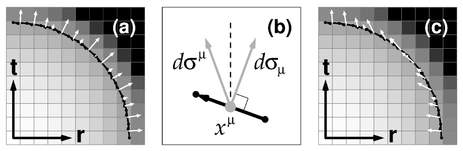
For instance, in 2D the history, i.e., the temporal evolution, of a temperature field of a one-dimensional (1D) relativistic fluid can be represented by a gray-level image (cf., Fig. 1). In the figure, we use the time and the radius for the temporal and the spatial dimensions, respectively. Let bright pixels (i.e., picture elements) refer to high temperatures and dark ones to low temperatures of the fluid. In this example, a 2D freeze-out hypersurface is an iso-therme.
In Fig. 1.a, we also depict the corresponding co-variant normal vectors . In 2D, the length of each normal vector is equal to the length of each supporting iso-contour vector. Each normal vector has its origin at the contra-variant center, , of a given contra-variant iso-contour vector and points to the exterior of the enclosed spacetime region. The latter is also indicated in Fig. 1.b, where we show that a contra-variant normal vector can be obtained by reflection of the co-variant normal vector at the time axis (dashed line).
Finally, in Fig. 1.c we show the contra-variant FO contour vectors with their corresponding contra-variant normal vectors . Not all of these contra-variant normal vectors point to the exterior of the enclosed spacetime region.
Note that the sign conventions of the normals of the transition hypersurface are important, and must be discussed, especially if both timelike and spacelike surfaces are studied. In fact, only the timelike contra-variant normal vectors point outwards, whereas the spacelike contra-variant normal vectors point inwards BRSnote .
If we know the FO hypersurface and the local momentum distribution after the transition the total, measurable momentum distribution can be evaluated by the Cooper-Frye formula CF74 .
III Equations for parameters of final matter in equilibrium
Let us define the contra-variant and co-variant surface normal four-vectors as
where in general , as the surface element can be either spacelike (-) or timelike (+). We can also introduce a unit normal to the surface as: so that Furthermore where for timelike surfaces and for spacelike surfaces . For the frequently used timelike, one-dimensional case .
In the general case the conserved energy-momentum current crossing the surface element is
| (6) |
must be continuous across the freeze-out surface, as must the baryon current ,
| (7) |
where is the invariant scalar baryon charge current.
We assume that the initial state, ””, and its energy momentum tensor and baryon current before the front is known. We aim for the characteristics of the final state. In total there are six unknowns in the equilibrated final state, these are , , and (here we drop the index ”” for the final state for shorter notation), however the pressure , a function of and , is given by the EoS, . Knowing and , the EoS, and the particular form of the corresponding equilibrated distribution function, the parameters , and , can also be obtained.
Thus, we have to solve 5 equations:
| (8) | |||||
| (9) | |||||
| (10) | |||||
| (11) | |||||
| (12) |
The l.h.s. represents quantities of the initial state of matter and the corresponding conserved quantities are known. Equations (9,10) can be solved for in the calculational frame:
| (13) |
Using now Eq. (10,11,12) one obtains , and in a similar fashion and
| (14) |
This results for , in
| (15) |
where, is an invariant scalar, and transforms as the 0-th component of the 4-vector . Notice that eq. (8) was not used up to this point, thus we can use there results both for the baryon-free and baryon-rich case.
We can have an elegant direct solution for the proper energy density, , and pressure, , as both of these quantities are invariant scalars, and we can express these by the covariant, 4-vector equation (6). From this 4-vector equation we can get two invariant scalar equations by (i) taking its norm, , and (ii) taking its projection to the normal direction, :
| (16) | |||||
| (17) |
Now expressing from eq. (17) and inserting it to eq. (16) , we obtain our final equation
| (18) |
which can be solved straightforwardly if the EoS, , is known. The other three elements of the equation, , , and , are known from the normal to the surface and from energy-momentum current from the pre-transition side.
Then, eqs. (13-15) can be used to determine the final flow velocity. At the end, after all conservation law equations are solved, we have to check the non-decreasing entropy condition (3) to see whether the solution is physically possible. If the overall entropy is decreasing after transition that would mean that the hypersurface is chosen incorrectly. One will need to choose more realistic condition for the transition and repeat the calculations.
This result can be used both if the initial state is in equilibrium and if it is not.
III.1 Final Matter with zero Baryon charge
In case of an ideal gas of massless particles after the front, with an EoS of , eq. (18) leads to a quadratic equation,
where , is the energy momentum transfer 4-vector across a unit hypersurface element.
If the flow velocity is normal to the FO hypersurface, , then for an initial perfect fluid in the Local Rest (LR) frame the above covariant equation takes a simple form,
This has two real roots, (energy density is conserved) and which does not correspond to a physical solution, as the energy density should not be negative.
III.2 Final Matter with Finite Baryon Charge
If the EoS depends on the conserved baryon charge density also, then we must exploit in addition eq. (7):
and inserting from here to eq. (17) yields
where is the generalized specific volume, well known from relativistic shock and detonation theory Cs94 . This equation provides another equation for as
| (19) |
which, together with eq. (18) and the EoS, , provide three equations to be solved for and .
This evaluation of the post FO configuration is in agreement with the theory of relativistic shocks and detonations Cs87 ; Ta48 allowing for both spacelike and timelike FO hypersurfaces. See also Cs94 . This method of evaluation observables is frequently used at the end of fluid dynamical model calculations (see e.g.Bravina ; Cs2009 ; Cs2010 ).
IV Transition to Molecular Dynamics before Freeze Out
Recently a frequently practiced method to describe the final stages of a reaction is to switch the FD model over to a Molecular Dynamics (MD) description at a transition hypersurface. This is frequently a fixed time, , or fixed proper time, hypersurface. The generation of the initial state of such an MD model is a task, which depends on the constituents of the matter described by the MD model. Nevertheless, same principles must be satisfied, like the conservation laws, eqs.(1-2).
IV.1 Equilibrium and EoS known before and after the transition
Let us assume, although not required by physical laws, that we have thermal equilibrium on both sides of the transition and we know explicitly the corresponding final momentum distribution of particles. Then, the fundamental equation to construct the post transition microscopic state, in addition to the conservation laws is the Cooper-Frye formula,
| (20) |
assuming that the local phase space distribution, , is known for all initial components of the MD model. If are local equilibrium distributions then (in principle) we know the intensive and extensive thermodynamical parameters and the EoS of the matter when the MD model simulation starts. These must not be the same as the ones before the transition hypersurface.
In the usual transition from FD to MD models, where the initial state of MD is in equilibrium, the EoS-s are known on both sides of the transition surface, and thus, both the equations of Rayleigh-line and Taub-adiabat, eqs. (5), as well as the invariant scalar equations derived here, eqs.(16,17,18,19) can be used to determine all parameters of the matter starting the MD simulation. These then determine the phase space distributions, of all components of the MD simulation. Subsequently eq.(20) can be used to generate randomly the initial constituents of the MD simulation.
As eq.(20) is a covariant equation applicable in any frame of reference, the most straightforward is to perform the generation of particles in the calculational frame of the MD model. This transition is by now performed in many hybrid models combining fluid dynamics with microscopic transport models BD1999 . These models at present are the most effective to describe experimental data and make the need for a Modified Boltzmann Transport Equation NW_layer less problematic.
In some cases the first step of the transition, the determination of the parameters of the final state from the exact conservation laws, is dropped with the argument that both before and after the transition the matter has the same constituents and the same EoS, thus the all extensive and intensive thermodynamical parameters as well as the flow velocity must remain the same. Then, using the intensive parameters the final particle distributions in the Cooper-Frye formula, eq.(20), can be directly evaluated in a straightforward way. This procedure is correct, but only if all features of the two states of the matter and their EoS are identical. In some cases the pre transition EoS assumes effective hadron masses depending on the matter density, while the final EoS is that of a hadron ideal gas mixture, but with fixed vacuum masses. This leads to a difference in the EoS, thus the above procedure is approximate. In such cases, the method can be used, but the accurate conservation laws can be enforced by a final adjustment step described in the next subsection.
The situation is similar if the constituents and the EoS are almost identical before and after the transition, but before the transition a weak or weakening mean field potential or compression energy is taken into account.
IV.2 Enforcing Conservation Laws with Approximate Generation of the Final State
In addition to the above mentioned approximate methods, even for really identical EoS-s across the transition or with generating the final EoS parameter based on conservation laws for the final EoS, inaccuracies may arise due to other reasons: during the random generation of the initial constituent particles of the MD simulation, the exact conservation laws may be violated, due to finite number effects. However, the energy and particle number conservations are usually enforced during the random generation of particles, even if the above procedure of solving the conservation laws beforehand is not fully followed. This is usually the consequence of the fact that the EoS of the MD model is not necessarily known if the model has complex constituents and laws of motion.
In any case to remedy this random error and make the conservation laws exactly satisfied a final correction step is advisable, and it is not always performed. If the energy and particle number conservations are enforced then, the last variable to balance is the momentum conservation. This regulates the flow velocity of the matter after the transition initiating the MD simulation.
The energy momentum tensor and baryon current for the generated random set of particle species, ”’, for each fluid cell (or group of cells if the multiplicity in a single cell is too low) can be calculated from the kinetic definition:
which, yield the resulting momentum and flow velocity of the matter. This can be used to adjust the flow velocity to achieve exact conservation of momentum, and modify the velocity of generated particles by the required Lorentz boost. The other conserved quantities may then be affected also, but an iterative procedure to eliminate the error completely is not crucial as the error can be given quantitatively.
If the randomly generated state is not following a thermal equilibrium phase space distribution, , and thus does not have an EoS, the above described scalar equations cannot be used to generate the initial configuration of the MD model. Nevertheless, the second step to check the conservation laws with the kinetic definition, and then correct the parameters of the generated particles can be done. For a required level of accuracy in this case an iterative procedure may be necessary.
Another, easier way to remedy this problem is to choose the transition hypersurface earlier so that the subsequent matter is still in thermal equilibrium. This can always be done if the requirement of entropy increase is satisfied.
V Final state out of thermal equilibrium
We have mentioned that the assumption for having thermal equilibrium in the final state is neither excluded nor required from transport theoretical considerations. However, thermal equilibrium distribution is not possible if we have to describe FO across a spacelike hypersurface (see the discussion in section I.)
In the MD model description the final post FO momentum distributions develope a local anisotropy if the FO has locally a preferred direction. Unless the unit normal of the FO hypersurface is equal to the local flow velocity of the pre FO matter, there is always a selected spatial direction which is the dominant direction of FO. This situation is discussed in several theoretical works, and some general features can be extracted from these studies.
V.1 Approximate kinetic models for Freeze Out
In explicit transport models this situation is handled Bu96 ; AC99-3309 ; Ta07 ; AL99-388 : starting from an equilibrium Jüttner distribution and considering a momentum dependent escape probability in the collision term, - which reflected the direction of the FO front and the distance from the front, - an anisotropic distribution was obtained (i.e. a distribution, which was anisotropic even in its own LR frame).
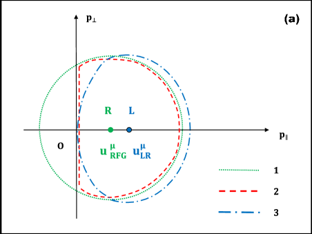
This anisotropic distribution could be approximated with analytic distribution functions Bu96 ; AC99-3309 : The starting point is the un-cut, isotropic, Jüttner distribution in the rest frame of the gas (RFG), which is centered around the 4-velocity vector, . This distribution is then cut or cut and smoothed. The resulting distribution has a different new flow velocity, , which is non-zero in RFG, and is pointing in space in the direction of the normal of the FO hypersurface, , labeled by . This defines the Local Rest (LR) frame of the post FO matter.
The spatial direction of is not affected by the Lorentz transformation from RFF to RFG and then to LR, as is the direction of the Lorentz transformation from RFG to LR 333In general the spatial components of the FO surface, , must not be parallel to or but these latter velocities can be decomposed to and components with respect to . Due to the construction Bu96 ; AC99-3309 ; Ta07 of the cut- or cancelling-Jüttner distributions or .. In the general case the boost in the direction leads to a change of the distribution function in the direction, but does not affect the distribution in the direction, or the procedure of cutting or cancelling the distribution in the direction. (The illustration in Fig. 2a shows the spatial momentum distribution where the boost in the orthogonal direction is already performed.)
In the final LR frame, the matter is characterized by a rather complex energy momentum tensor, inheriting some parameters from the original uncut distribution in RFG, like the temperature and chemical potential, but as the resulting distribution is not a thermal equilibrium distribution, these parameters are not playing any thermodynamical role. One has to determine all parameters numerically from conservation laws (1,2), as done in refs. AC99-3309 ; Ta07 .
Interestingly, a simplified numerical kinetic FO model AL99-388 led to a FO distribution satisfying the condition for spacelike FO with a smooth distribution function, which is anisotropic (also in its own LR frame) and has a symmetry axis pointing in the dominant FO direction. This distribution was then approximated with an analytic, ”cancelling-Jüttner” distribution Ta07 , which can also be used to solve the FO problem.
After FO, the symmetry properties of the energy momentum tensor are the same for the cut-Jüttner and cancelling-Jüttner cases Bu96 ; AC99-3309 ; Ta07 . The FO leads to an anisotropic momentum distribution and therefore to an anisotropic pressure tensor. The energy momentum tensor is not diagonal in the RFG frame, there is a non vanishing transport term, AC99-3309 ; Ta07 , in the 2-dimensional plane spanned by the 4-vectors, and . One can, however, diagonalize the energy momentum tensor by making a Lorentz boost into the LR frame using Landau’s definition for the 4-velocity, . In this frame then the energy momentum tensor becomes diagonal, but the pressure terms are not identical, due to the anisotropy of the distribution:
| (21) |
Here the energy density, , of course must not be the same as in the case of an isotropic, thermal equilibrium post FO momentum distribution. This can be seen from the kinetic definition of the energy momentum tensor as shown in refs. AC99-3309 ; Ta07 .
We need the complete post FO momentum distribution and the corresponding energy momentum tensor to determine final observables. This depends on the transport processes at FO, and cannot be given in general; however, due to the symmetries of the collision integral, the symmetries of the energy momentum tensor are the same irrespectively of the ansatz used (e.g. cut-Jüttner, cancelling-Jüttner or some other distribution).
In kinetic transport approaches the microscopic escape probability MC0607 is peaking in the direction of , which yields a distribution peaking in this direction, i.e. yielding the same symmetry properties as the previously mentioned analytic ansatzes. The energy momentum tensor in general takes the form
| (22) |
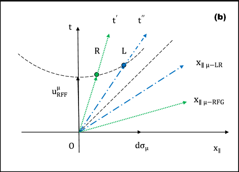
where is the orthogonal projector to , and is the unit 4-vector projection of in the direction orthogonal to , i.e. , where ensures normalization to -1. In the Landau LR frame this returns expression (21). The 4-velocity, , and the other parameters of the post FO state of matter, should be determined from the conservation laws (1,2). The schematic diagram of the asymmetric distributions and the different reference frames can be seen in Fig. 2.
The FO problem was solved for these configurations and ansatzes, by satisfying the conservation laws explicitly for the full energy momentum tensor. We do not have a general EoS(s) that would characterize the connection among , and , furthermore the relation connecting these quantities depends on the 4-vectors and . In addition this connection depends on the details or assumptions of the transport model. The simple models AC99-3309 ; Ta07 provide examples for such a dependence. If is known, then for baryon free matter we can determine four unknowns: and, an additional parameter of the post FO distribution, from eq. (2). (Due to normalization only 3 components of are unknowns.) For baryon-rich matter we can determine one more unknown parameter, since we have one additional equation, the conservation of baryon charge from eq. (1).
V.2 Exploiting general symmetries of anisotropic final states
The first step of solution can be done similarly to the isotropic case. Then in eq. (6) the enthalpy will change as , and , plus an additive term will appear, . Furthermore, eqs. (9-12) remain of the same form, with , and , plus the additive term will appear in the r.h.s. of eqs.(9-12). This additive term will also appear in the expression of after eq. (13) and in the denominator of eq. (15) also.
The additional term, , in eq. (6) is orthogonal to (by definition of ), so when we calculate the scalar product (16) their cross term vanishes, so
| (23) | |||||
| (24) | |||||
Now one can express from eq. (24) and inserting it to eq. (23), we obtain that
| (25) |
where this equation is not a scalar equation as it dependes on , where the projector is dependent on . These equations are similar to the ones obtained for the isotropic case, however, to solve this last equation we need a more complex relation among , , . As these arise from the collision integral in the BTE approach the needed relation may depend on and . On the other hand, the escape probability may be simple, or may be approximated in a way, which yields an ansatz for this relation with adjustable parameters, and then the problem is solvable. This was the case in refs. MC0607 ; NW_layer .
The recent covariant formulation of the kinetic freeze-out description MC0607 indicates that the relation among the different parameters of the anisotropic energy momentum tensor, should be possible to express in terms of invariant scalars, which may facilitate the solution of the anisotropic FO problem.
When the adjustable parameters of the post FO matter are determined in this way from the conservation laws, we still need the underlying anisotropic momentum distribution of the emitted particles in order to evaluate the final particle spectra using the Cooper-Frye formula with this anisotropic distribution function. Once again, when all conservation law equations are solved we have to check the non-decreasing entropy condition to see whether the selected FO hypersurface is realistic.
In case of an anisotropic final state, due to the increased number of parameters and their more involved relations, the covariant treatment of the problem may not provide a simplification, compared to the direct solution of conservation laws for each component of the energy momentum tensor (e.g. AC99-3309 ; Ta07 ).
V.3 Anisotropic initial and final states
Recent viscous fluid dynamical calculations evaluate the anisotropy of the momentum distribution is in the pre FO viscous flow (see e.g. MoHu09 .) This anisotropy is governed by the spacetime direction of the viscous transport. The pre and post FO matter may still be different, e.g. the pre FO state may be viscous QGP with current quarks and perturbative vacuum, while post FO we may have a hadron gas or constituent quark gas. The final state will also be anisotropic, not only because of the initial anisotropy but also due to freeze-out. The two physical processes leading to anisotropy are independent, so their dominant directions are in general different. In this case the general symmetries are uncorrelated and cannot be exploited to simplify the description of the transition. Due to the change of the matter properties, the conservation laws, eqs. (1-3), are needed to determine the parameters of the post FO matter before the Cooper-Frye formula with non-equilibrium post FO distribution is applied to evaluate observables.
VI Summary
In this work a new simple covariant treatment is presented for solving the conservation laws across a transition hypersurface. This leads to a significant simplification of the calculation if both the initial and final states are in thermal equilibrium. The same method can also be used for the more complicated anisotropic final state, however, this method is only advantageous if the more involved relations among the parameters of the post FO distribution and the distribution itself is given in covariant form, preferably through invariant scalars.
References
- (1) L. D. Landau, Izv. Akad. Nauk SSSR 17 (1953) 51.
- (2) G. Milekhin, Zh. Eksp. Teor. Fiz. 35 (1958) 1185; Sov. Phys. - JETP 35 (1959) 829; and G. A. Milekhin, Trudy FIAN 16 (1961) 51.
- (3) F. Cooper and G. Frye, Phys. Rev. D, 10 (1974) 186.
- (4) G.F. Chapline, M.H. Johnson, E. Teller and M.S. Weiss, Phys. Rev. D8 (1973) 4302
- (5) W. Scheid, H. Müller and W. Greiner, Phys. Rev. Lett. 32 (1974) 741.
- (6) L. P. Csernai, Sov. JETP 65 (1987) 216; Zh. Eksp. Theor. Fiz. 92 (1987) 379.
- (7) L. P. Csernai: Introduction to Relativistic Heavy Ion Collisions (Wiley, New York, 1994).
- (8) A. H. Taub, Phys. Rev. 74 (1948) 328.
- (9) V.K. Magas, L.P. Csernai, D.D. Strottman, Phys. Rev. C64 (2001), 014901, and V.K. Magas, L.P. Csernai, D.D. Strottman, Nucl. Phys. A 712 (2002) 167.
- (10) K. A. Bugaev, Nucl. Phys. A 606 (1996) 559.
- (11) Cs. Anderlik, L. P. Csernai, F. Grassi, W. Greiner, Y. Hama, T. Kodama, Zs. I. Lazar, V. K. Magas, and H. Stöcker, Phys. Rev. C 59 (1999) 3309.
- (12) K. Tamosiunas, L. P. Csernai. Eur. Phys. J. A20 (2004) 269.
- (13) Cs. Anderlik et al., Phys. Rev. C 59 (1999) 388; V. K. Magas et al., Heavy Ion Phys. 9, 193 (1999); Phys. Lett. B 459, 33 (1999); Nucl. Phys. A 661, 596 (1999).
- (14) V. K. Magas, A. Anderlik, C. Anderlik and L. P. Csernai, Eur. Phys. J. C 30, 255 (2003)
- (15) E. Molnar, L. P. Csernai, V. K. Magas, A. Nyiri, K. Tamosiunas, Phys. Rev. C74, 024907 (2006); J. Phys. G 34 (2007) 1901; E. Molnar, L. P. Csernai and V. K. Magas, Acta Phys. Hung. A 27, 359 (2006); V. K. Magas, L. P. Csernai and E. Molnar, Acta Phys. Hung. A 27, 351 (2006).
- (16) V. K. Magas, L. P. Csernai and E. Molnar, Eur. Phys. J. A 31, 854 (2007); Int. J. Mod. Phys. E 16, 1890 (2007); V. K. Magas and L. P. Csernai, Phys. Lett. B 663, 191 (2008);L.P. Csernai, V.K. Magas, E. Molnar et al., Eur. Phys. J. C 25, 65 (2005);V.K. Magas, L.P. Csernai, E. Molnar et al., Nucl. Phys. A 749, (2005).
- (17) F. Grassi, Y. Hama, S. S. Padula, and O. Socolowski, Phys. Rev. C 62 (2000) 044904.
- (18) B. R. Schlei, “A new computational framework for 2D shape-enclosing contours,” Image and Vision Computing 27 (2009) 637, doi: 10.1016/j.imavis.2008.06.014.
- (19) B. R. Schlei, “VESTA - Surface Extraction,” Theoretical Division - Self Assessment, Special Feature, a portion of LA-UR-03-3000, Los Alamos (2003) 37.
- (20) B. R. Schlei, “Hyper-Surface Extraction in Four Dimensions,” Theoretical Division - Self Assessment, Special Feature, a portion of LA-UR-04-2143, Los Alamos (2004) 168.
- (21) B. R. Schlei, “Volume-Enclosing Surface Extraction,” in preparation.
- (22) Note, that we actually use for hypersurface construction in 1+1, 2+1, and 3+1 dimensional numerical simulations the corresponding computer codes, i.e., DICONEX, VESTA, and STEVE, respectively. Ref. BRS09 explains in great detail the extraction of an oriented FO contour which is represented by a set of contra-variant (so-called “DICONEX iso-contour”) vectors. In 2D, the simplices which represent a hypersurface best are line segments, whereas in 3D and 4D they are triangles BRS03 ; BRS10 and tetrahedrons BRS04 , respectively. In particular, the contra-variant 2D FO contour vectors are oriented counter-clockwise around the enclosed spacetime regions. The co-variant normals of the contra-variant simplices are obtained from calculating the mathematical duals of these simplices with respect to a geometric product (cf., e.g., Ref. CP09 ) within the N-dimensional multi-linear space under consideration. Note, that the co-variant normal vectors do not depend on any given metric tensor, whereas the contra-variant normal vectors do BRS10 .
- (23) C. Perwass, Geometric Algebra with Applications in Engineering, Geometry and Computing, Springer, 2009.
- (24) L. Bravina, L.P. Csernai, P. Lévai, and D. Strottman, PRC 50 (1994) 2161.
- (25) L.P. Csernai, Y. Cheng, Sz. Horvát, V. Magas, D. Strottman and M.Zétényi, J. Phys. G 36 (2009) 064032.
- (26) L.P. Csernai, Y. Cheng, V.K. Magas. I.N. Mishustin and D. Strottman, Nucl. Phys. A 834 (2010) 261c.
- (27) S.B. Bass, A. Dumitru, M. Bleicher et al., Phys. Rev. C60, 021902 (1999); D. Teaney, J. Lauret and E.V. Shuryak, Nucl. Phys. A 698, 479 (2002); S.A. Bass, T. Renk, J. Ruppert et al., J. Phys. G 34, S979 (2007); C. Nonaka, M. Asakawa and S.A. Bass, J. Phys. G 35, 104099 (2008); H. Petersen, J. Steinheimer, G. Burau, M. Bleicher, H. Stöcker, Phys. Rev. C 78 (2008) 044901; T. Hirano and Y. Nara, Phys. Rev. C 79, 064904 (2009).
- (28) P. Huovinen and D. Molnar, Phys. Rev. C 79 (2009) 014906.