Semiclassical quantization of skipping orbits

Abstract

We propose a simple description of the spectrum of edge states in the quantum Hall regime, in terms of semiclassical quantization of skipping orbits along hard wall boundaries, ${\cal A}=2\pi(n+\gamma)\ell_{B}^{2}$, where ${\cal A}$ is the area enclosed between a skipping orbit and the wall and $\ell_{B}$ is the magnetic length. Remarkably, this description provides an excellent quantitative agreement with the exact spectrum. We discuss the value of $\gamma$ when the skipping orbits touch one or two edges, and its variation when the orbits graze the edges and the semiclassical quantization has to be corrected by diffraction effects. The value of $\gamma$ evolves continuously from $1/2$ to $3/4$. We calculate the energy dependence of the drift velocity along the different Landau levels. We compare the structure of the semiclassical cyclotron orbits, their position with respect to the edge, to the wave function of the corresponding eigenstates.

I Introduction

The edge states play a crucial role for understanding the integer and fractional quantum Hall effects. Their description has been introduced in the seminal paper by Halperin. Halperin82 ; MacDonald84 This picture has then been elaborated by Buttiker Buttiker88 and a review can be found in ref. [review, ]. It appears often convenient to picture qualitatively these edge states in terms of skipping cyclotron orbits. But the link between the full quantum mechanical treatment of the states and this qualitative picture is missing (see however ref. [Beenakker89, ]). Here we propose an extensive development of this picture and show how the semiclassical quantization of these orbits leads to a qualitative and even quantitative description of the edge states energy levels.

We consider a free electron (mass $m$, charge $-e$) moving in a ribbon infinite along the $y$ direction and bounded along the $x$ direction. A magnetic field $B$ is applied along $z$. As in ref. [Halperin82, ], we consider the situation where the confining potential consists in an abrupt potential well of infinite height. This is known not to be the correct situation in the two-dimensional electron gas of $GaAs$ heterostructures, where the confining potential is rather smooth at the scale of the magnetic length $\ell_{B}$. However, we believe that the case of the abrupt potential is interesting in itself and may be relevant to other related situations exhibiting edge states. For example, graphene ribbons have sharp boundaries which must be modeled with sharp potentials.BreyFertig ; Delplace We comment the case of smooth boundaries at the end of the paper. Far from the edges, the energy levels are given by $E_{n}=(n+1/2)\hbar\omega_{c}$ where $\omega_{c}=eB/m$ is the cyclotron frequency. This Landau quantization can be obtained quite easily from the Bohr-Sommerfeld quantization rule that we recall below. The goal of this work is to describe the semiclassical motion of the electron near one edge, described here by a ”hard wall”, that is an infinite potential well. We consider the vicinity of the edge located at $x=0$, assuming first that the second edge is far away ($x\rightarrow-\infty$).

The problem is solved semiclassically by quantization of the action. In the appropriate gauge, the well-known Landau problem is related to the problem of a one-dimensional oscillator. In the presence of a sharp edge, the problem to be solved is the one of an harmonic oscillator in the presence of an infinite potential well. This problem is solved by quantization of the semiclassical action $S(E)=2\pi(n+\gamma)\hbar$, where $\gamma$ is related to a so-called Maslov index.Maslov For the free oscillator, $\gamma=1/2$ corresponds to the sum of two contributions $\gamma_{i}=1/4$ of the two turning points. In the presence of the potential well, $\gamma$ evolves from $1/2$ to $3/4$ when the guiding center $x_{c}$ of the cyclotron orbit (the center of the harmonic oscillator) approaches the wall. A form of the continuous variation $\gamma_{n}(x_{c})$ for a given $n$ has been recently obtained.Avishai08

In this paper, we give a very simple description of the edge states spectrum in terms of quantization of skipping orbits. This image, currently used in the literature or in pedagogical presentations, has curiously never been described in details (see however ref. [Beenakker89, ]). Yet, it leads to a number of results which to our knowledge have never been discussed. In the next section, we recall the mapping, in the Landau gauge, to a one-dimensional problem of a harmonic oscillator and we calculate the action $S(E)$ of this oscillator. In section III, we give a complete picture of the evolution of the energy levels in terms of the quantization of the area of skipping orbits. The well-known quantization of closed orbits can be extended to the case of skipping orbits. Then, their area depends on the distance $x_{c}$ to the wall and must be quantized as

$${\cal A}(R,x_{c})=2\pi(n+\gamma)\ell_{B}^{2}$$ (1)

where $\ell_{B}$ is the magnetic length, $R$ is the cyclotron radius and $x_{c}$ is the position of the guiding center with respect to the wall. This well-known quantization rule for closed orbits appears to be also valid for open but periodic skipping orbits. Using the same method, we calculate in section IV the full spectrum in the case a ribbon, when the magnetic length is of the order of the width of the ribbon so that the two edges have to be considered. Then we conclude in section V, with a comparison with the case of a smooth potential.

II Mapping to a one-dimensional oscillator

The problem to be solved is described by the Hamiltonian

$${\cal H}={p_{x}^{2}\over 2m}+{p_{y}^{2}\over 2m}+V(x)$$ (2)

where the potential $V(x)$ describes the edge of the sample along the $y$ direction. We choose $V(x)=0$ when $x<0$ and $V(x)=\infty$ when $x>0$. Using the Landau gauge ${\bm{A}}=(0,Bx,0)$, the corresponding eigenvalue problem reads ($-\infty<x\leq 0$) :

$$[-{\hbar^{2}\over 2m}{d^{2}\over dx^{2}}+{1\over 2}m\omega_{c}^{2}(x_{c}-x)^{2}]\psi(x)=E\psi(x),$$ (3)

with the constraint $\psi(0)=0$. The center $x_{c}$ of the oscillator, is related to the $k_{y}$ component of the wave vector which is a good quantum number: $x_{c}=k_{y}\ell_{B}^{2}$ where $\ell_{B}=\sqrt{\hbar/eB}$ is the magnetic length. The action $S$ along a closed trajectory is given by $S=\oint p_{x}dx=2\int p_{x}dx$ where, far from the edge (region I in Fig. 1) factor2

$$S =2\int_{x_{c}-R}^{x_{c}+R}\sqrt{2mE-m^{2}\omega_{c}^{2}(x-x_{c})^{2}}dx$$ (4)

$$={2\pi E\over\omega_{c}}={\pi}m\omega_{c}R^{2}.$$

$R(E)=\sqrt{2E/m\omega_{c}^{2}}$ is the cyclotron radius of the classical trajectory and $x_{c}\pm R$ are the positions of the turning points. The semiclassical quantization of the action

$$S(E)=2\pi(n+\gamma)\hbar$$ (5)

leads to the energy quantization,

$$E=(n+\gamma)\hbar\omega_{c}$$ (6)

where the value $\gamma=1/2$ is not given by the semiclassical quantization rule and results from the matching of the wave function at the two turning points.

When the cyclotron orbit approaches the edge, that is when the center $x_{c}$ of the cyclotron orbit becomes larger than $-R$ (energy regions IIa and IIb in Fig. 1), the turning points are located at $x_{1}=x_{c}-R$ and $x_{2}=0$. The action now explicitly depends on $x_{c}$ and it is given by factor2

$$S(E,x_{c}) = 2\int_{x_{c}-R}^{0}\sqrt{2mE-m^{2}\omega_{c}^{2}(x-x_{c})^{2}}dx$$ (7)

$$= {2E\over\omega_{c}}[{\pi\over 2}-\arcsin{x_{c}\over R}-{x_{c}\over R}\sqrt{1-x_{c}^{2}/R^{2}}].$$

Introducing the angle $\theta$ such that $\cos\theta=x_{c}/R$, the action can be rewritten as

$$S(E,x_{c})={E\over\omega_{c}}[2\theta-\sin 2\theta]={1\over 2}m\omega_{c}R^{2}[2\theta-\sin 2\theta]\ .$$ (8)

We give in the next section a very simple interpretation of this angle $\theta$. The energy levels $E_{n}(x_{c})$ are still given by quantization of the action (5) which now depends on the position with respect to the wall. When $x_{c}>-R$, the factor $\gamma$ is equal to $3/4$, because it results from different matching conditions at the two turning points. At the left turning point $\gamma_{l}=1/4$, while at the right turning point, the vanishing of the wavefuntion implies $\gamma_{r}=1/2$, so that $\gamma=\gamma_{l}+\gamma_{r}=3/4$. $\gamma$ evolves between $1/2$ and $3/4$ when $x_{c}\simeq-R$.

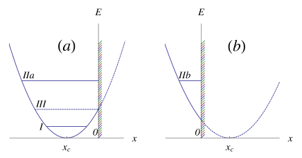
Figure 1: $1D$ harmonic oscillator centered on $x_{c}$, with an infinite potential well in $x=0$. a) The guiding center is inside the sample. b) The guiding center is outside the sample. Three distinct regions have to be considered : I : the energy levels are not affected by the edge and $\gamma=1/2$, II: the trajectories hit the edge and $\gamma=3/4$. In between, the phase factor $\gamma$ evolves between $1/2$ and $3/4$. It is $2/3$ when the cyclotron orbit just grazes the wall (III).

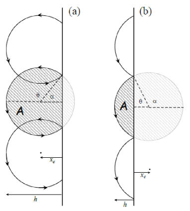
Figure 2: Semiclassical skipping orbits a) when the guiding center is inside the sample (region IIa in Fig. 1); b) when it is outside (region IIb in Fig. 1). The dashed area ${\cal A}$ is quantized as ${\cal A}=2\pi(n+\gamma)\ell_{B}^{2}$.

III Quantization of skipping orbits

III.1 Quantization of the area

The quasiclassical Bohr-Sommerfeld quantization rule for skipping orbits has been discussed by Beenakker and Van Houten Beenakker89 . Since the motion along the $x$ axis is periodic, this quantization rule can be written as

$$S=\oint p_{x}\cdot dx=2\pi(n+\gamma)\hbar\ .$$ (9)

where ${\bm{p}}=m{\bm{v}}-e{\bm{A}}$. The trajectories are now open and the notation $\oint$ means that the integral is taken along one period of the motion. The gauge for the vector potential ${\bm{A}}$ must be chosen such that $A_{x}$ is periodic. The simplest choice is $A_{x}=0$, so that $p_{x}=mv_{x}$. The classical equation of motion for the $x$ component of the velocity is $v_{x}=-\omega_{c}(y-y_{0})$ where $y_{0}$ is an arbitrary position. Therefore the quantization condition (9) becomes

$$m\oint v_{x}dx=-eB\oint(y-y_{0})dx=2\pi(n+\gamma)\hbar\ .$$ (10)

The integral is nothing but the area ${\cal A}$ enclosed between one arc of the periodic orbit and the wall (see Fig. 2). Therefore we can generalize the familiar quantization rule (1) of the area ${\cal A}$ to the case of skipping orbits. This area can be parametrized by the angle $\theta$ shown in Fig. 2 and defined by $x_{c}=R\cos\theta$. We have

$${\cal A}(E,x_{c})={R^{2}\over 2}[2\theta-\sin 2\theta]$$ (11)

which is precisely the same equation (8) as obtained in the 1D picture. Then the quantization of the area ${\cal A}$ reads

$${\cal A}(R,x_{c})=2\pi(n+\gamma)\ell_{B}^{2}$$ (12)

so that the angle $\theta$ can be used to parametrize the solutions ($\theta=\pi$: the orbit just grazes the edge, $x_{c}=-R$. $\theta=\pi/2$: the guiding center of the orbit in precisely on the edge. $\theta<\pi/2$: the center of the orbit stands outside the sample). From equations (11,12), we obtain

$$R^{2}={4\pi(n+\gamma)\ell_{B}^{2}\over 2\theta-\sin 2\theta}$$ (13)

and the energy levels are given by

$$E=\hbar\omega_{c}{R^{2}\over 2\ell_{B}^{2}}=\hbar\omega_{c}(n+\gamma){2\pi\over 2\theta-\sin 2\theta}$$ (14)

The cyclotron radius $R$ is related to the position $x_{c}$ of the guiding center:

$$x_{c}=R\cos\theta=\ell_{B}\sqrt{4\pi(n+\gamma)\over 2\theta-\sin 2\theta}\cos\theta$$ (15)

so that the dependence $E_{n}(x_{c})$ is simply parametrized by the angle $\theta$. However, the main complexity of the problem comes from the fact that $\gamma$ is not a constant. It is fixed to the value $1/2$ far from the edge, but on the other hand, for skipping orbits, it reaches the value $3/4$. Therefore, from the quantization condition (12), we obtain two branches (Fig. 3).

III.2 Spectrum

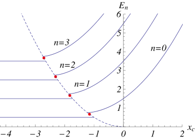
Figure 3: Energy levels obtained from semiclassical quantization of the area ${\cal A}(E,x_{c})=2\pi(n+\gamma)\ell_{B}^{2}$. Inside the sample ($x_{c}<<-R$), $\gamma=1/2$. For skipping orbits ($x_{c}>>-R$), $\gamma=3/4$. The dashed line corresponds to $x_{c}=-R$, the case where the cyclotron orbit just touches the edge. In this case, we have found that $\gamma=2/3$ and the position of the energy levels is marked with small dots along the dashed line. The energy levels are plotted in units of $\hbar\omega_{c}$ and the distance $x_{c}$ is plotted in units of $\ell_{B}$.

In the intermediate region, when the cyclotron orbit is very close to the wall, that is when $x_{c}\simeq-R$, $\gamma$ varies continuously between $1/2$ and $3/4$. This regime has been studied recently within a WKB approach.Avishai08 In particular, when the cyclotron orbit strictly touches the wall $x_{c}=-R$, it has been found that the parameter $\gamma=2/3$. This factor comes from a contribution $1/4$ on the left side and a very peculiar and new contribution $5/12$ from the right side, which, to our knowledge has never been studied, at least in this context. Moreover, in ref. [Avishai08, ], we have found an interpolation formula for $\gamma_{n}(x_{c})$ for a given value of $n$. It is given by

$$\gamma_{n}(x_{c})={1\over 2}\ {1+3e^{AX}\over 1+2e^{AX}}$$ (16)

where $X=(2n+4/3)^{1/6}(x_{c}/\ell_{B}+\sqrt{2n+4/3})$ and $A\simeq 3.5$. This expression can be extended by transforming it into a function of energy and $x_{c}$ : $\gamma(E,x_{c})$ is still given by Eq. (16), with $X=(2E/\hbar\omega_{c})^{1/6}(x_{c}/\ell_{B}+\sqrt{2E/\hbar\omega_{c}})$. It can be actually decomposed in the form

$$\gamma(E,x_{c})={1\over 2}+\gamma_{r}(E,x_{c})$$ (17)

since it is known to be the contribution of two terms corresponding respectively to the left and to the right turning points. We have

$$\gamma_{r}(E,x_{c})={1\over 4}\ {1+4e^{AX}\over 1+2e^{AX}}$$ (18)

Given these expressions and the implicit equation (12), the full spectrum is obtained in Fig. 4.

The scenario when the cyclotron orbits approaches the edge is the following. When $x_{c}\ll-R$, that is far from the edge, the cyclotron radius is $R=\ell_{B}\sqrt{2n+1}$. When the distance between the orbit and the edge becomes of order of the magnetic length $\ell_{B}$, the energy and the cyclotron radius start to increase to reach the values $E_{n}=(n+2/3)\hbar\omega_{c}$ and $R=\ell_{B}\sqrt{2n+4/3}$ when the cyclotron orbit just touches the edge. Then the energy and the cyclotron radius continue to increase as shown in Fig. 4.

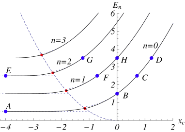
Figure 4: Black curves: Energy levels obtained from semiclassical quantization of the area ${\cal A}(E,x_{c})=2\pi(n+\gamma_{n}(x_{c}))\ell_{B}^{2}$, where we have used the expression (16) for $\gamma_{n}(x_{c})$. The dashed line corresponds to $x_{c}=-R$, the case where the cyclotron orbit just touches the edge. On this line, $\gamma=2/3$. The dotted lines are the approximation of a constant $\gamma=1/2$ or $3/4$, see Fig. 3. The large dots indicate special points where the wave function can be easily obtained from the solution of the harmonic oscillator in free space (see Figs. 6,7). When $x_{c}\simeq-R$, $\gamma$ varies continuously between $1/2$ and $3/4$ so that the spectrum is continuous. The energy levels are plotted in units of $\hbar\omega_{c}$ and the distance $x_{c}$ is plotted in units of $\ell_{B}$.

It is also interesting to introduce the position ${h}$ of the extremum of the cyclotron orbit (Fig. 2), that is the position of the left turning point in the $1D$ picture. It is ${h}=-2R$ when the cyclotron orbit just touches the edge and it varies to ${h}\rightarrow 0$ when $x_{c}\rightarrow\infty$. A simple geometric picture shows that ${h}=x_{c}-R=R(\cos\theta-1)<0$, that is, using 13:

$${h}=R(\cos\theta-1)=\ell_{B}\sqrt{4\pi(n+\gamma)\over 2\theta-\sin 2\theta}(\cos\theta-1)$$ (19)

In Fig. 5, we plot the energy as a function of the position ${h}$. Of course, $x_{c}$ can increase to infinity and ${h}$ stays confined to the inside of the sample (${h}<0$). (cf. inflexion point).

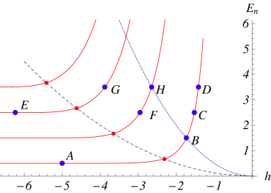
Figure 5: Energy levels $E_{n}({h})$ obtained from semiclassical quantization. ${h}$ is the position of the extremum of the cyclotron orbit. The dashed line corresponds to ${h}=-2R$, the case where the cyclotron orbit just touches the edge. On this line, $\gamma=2/3$. The dotted line corresponds to ${h}=-R$, that is $x_{c}=0$. The large dots indicate special points where the wave function can be easily obtained from the solution of the harmonic oscillator in free space (see figures 6,7). The energy levels are plotted in units of $\hbar\omega_{c}$ and the distance ${h}$ is plotted in units of $\ell_{B}$

The large dots marked in Figs. 4,5 correspond to simple cases where the energy and the wave function are easily known. For these special points, where the energy is the same as in free space ($3/2,5/2,7/2\times\hbar\omega_{c}$), the wave function is also the same as in free space but must vanish in $x=0$. The wave functions in free space are well known to be related to the Hermite functions. Therefore the edge must coincide with a zero of these Hermite functions. For example the points $B$ and $H$ correspond to antisymmetric wave functions, that is to energies $E_{n}=E_{2p+1}=\hbar\omega_{c}(2p+3/2)$. In Fig. 6, we have shown the evolution of the normalized squared wavefunction $|\psi(x)|^{2}$ for increasing values of $x_{c}$. In Fig. 7, we show three wave functions with energy $5/2\hbar\omega_{c}$, having respectively $two$, $one$ and no zeroes. In these two figures, one sees that the extension of the wave function is given by the extremum of the classical skipping orbit.

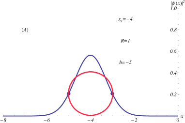
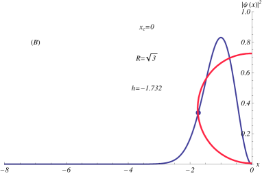
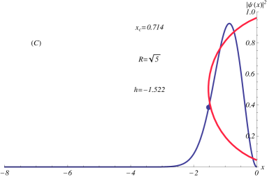
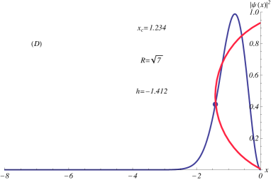
Figure 6: Evolution of the ground state wave function ($n=0$) when the position $x_{c}$ of the guiding center approaches and crosses the edge. The four cases correspond to the points (A), (B), (C) and (D) shown in Figs. 4,5. The position of the turning point (at distance $|{h}|$ from the edge) is marked with a dot. Is is seen that the extension of the wave function is given by the extremum of the classical skipping orbit. The distance $x$ is plotted in units of $\ell_{B}$.

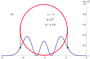
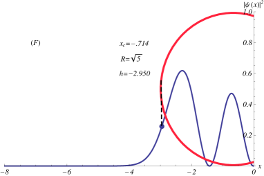
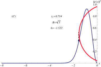
Figure 7: Evolution of the state of energy $5/2\hbar\omega_{c}$ when $x_{c}$ increases, corresponding to the points (E), (F) and (C) shown in Figs. 4,5. The extension of the wave function is given by the extremum of the semiclassical orbit. Distances are in units of $\ell_{B}$.

III.3 Drift velocity

We now calculate semiclassically the drift velocity along an edge state at a given energy $E$. The cyclotron radius is $R=\sqrt{2E/m\omega_{c}^{2}}$ and the velocity along the cyclotron orbit is given by $v_{E}=\omega_{c}R=\sqrt{2E/m}$. The length of the skipping orbit being $2R\theta$ (Fig. 2), the period $T$ is given by

$$T=2R\theta/v={2\theta\over\omega_{c}}\ .$$ (20)

Classically, the drift velocity $v_{d}^{cl}$ along the $y$ direction can be easily obtained from simple geometry (Fig. 2), the distance between two successive hits on the edge being $2R\sin\theta$:

$$v_{d}^{cl}={2R\sin\theta\over T}=\omega_{c}R{\sin\theta\over\theta}=v_{E}{\sin\theta\over\theta}$$ (21)

It is interesting to compare this value to the drift velocity obtained from the energy

$$v_{d}={\partial E\over\hbar\partial k_{y}}={1\over eB}{\partial E\over\partial x_{c}}$$ (22)

which is the correct result, beyond semiclassical approximation. The derivative can be calculated from Eqs. (14, 15), and one recovers the classical expression (21) provided $\gamma$ is a constant. However in the region where the cyclotron orbit is near the edge $x_{c}\simeq-R$, $\gamma$ varies continuously between $1/2$ and $3/4$. A better evaluation of the drift velocity is obtained in the WKB approximation which accounts for the variation of $\gamma$ (Eq. 16). The energy levels are given by the two equations

$$R^{2}={4\pi[n+\gamma_{n}(x_{c})]\over 2\theta-\sin 2\theta}\ell_{B}^{2}\qquad,\qquad x_{c}=R\cos\theta$$ (23)

Since $E=\hbar\omega_{c}R^{2}/2\ell_{B}^{2}$, the drift velocity is

$$v_{d}^{WKB}={1\over eB}{\partial E\over\partial x_{c}}=\omega_{c}R{\partial R\over\partial x_{c}}$$ (24)

By differentiating Eqs. (23), and eliminating $\partial R/\partial\theta$, we obtain

$$v_{d}^{WKB}=\omega_{c}R{\sin\theta\over\theta}+2\pi\omega_{c}\ell_{B}^{2}{\sin^{2}\theta\over\theta(1-\cos 2\theta)}{\partial\gamma_{n}\over\partial x_{c}}$$ (25)

The derivative $\partial\gamma_{n}\over\partial x_{c}$ is non zero only in the vicinity $x_{c}\simeq-R$, in which case the angle $\theta$ is very close to $\pi$. Therefore, in a very good approximation, we obtain:

$$v_{d}^{WKB}=v_{d}^{cl}+\omega_{c}\ell_{B}^{2}{\partial\gamma_{n}\over\partial x_{c}}\ .$$ (26)

The dependence $v_{d}^{WKB}(x_{c})$ is plotted in Fig. (8) and is compared to the numerical fully quantum calculation. The drift velocity, which is zero inside the sample, starts to increase when the cyclotron orbit touches the edge. The WKB approximation is excellent except close to the point where the classical cyclotron orbit just touches the boundary. When the skipping orbit gets closer and closer to the edge, the energy increases and the classical approximation (21) becomes excellent.

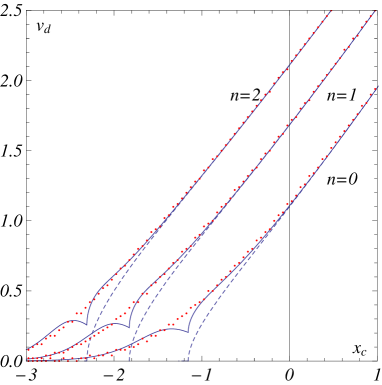
Figure 8: Variation of the drift velocity $v_{d}$ (in units of $\hbar/m\ell_{B}$) with the position $x_{c}$ for the three lowest energy levels. Red dots: exact numerical calculation; full line: result (26) of the WKB calculation; dashed line: classical drift velocity (21). $x_{c}$ is in units of $\ell_{B}$.

Fig. 9 represents the drift velocity normalized to the Fermi velocity, as a function of the energy along a given edge state. The drift velocity ultimately saturates towards the Fermi velocity at high energy.

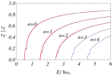
Figure 9: Variation of the drift velocity with the energy along different Landau levels. The drift velocity is normalized to the Fermi velocity $v_{E}$ corresponding to energy $E$. The full lines are the WKB calculations and the dots are the exact results.

.

IV Two edges

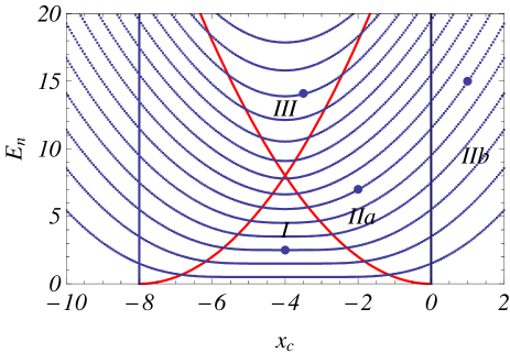
Figure 10: Landau levels spectrum calculated numerically for a ribbon of finite width $d=8\ell_{B}$. The two vertical lines indicate the position of the edges and the two parabolas indicate the positions $x_{c}$ for which the classical orbits touch the edges, $x_{c}=-R$ and $x_{c}=-d+R$. $x_{c}$ is written in units of $\ell_{B}$.

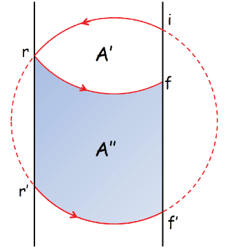
Figure 11: In the presence of two walls, the area delimited by a periodic trajectory in the area ${\cal A}^{\prime}$, but the area ${\cal A}$ to be quantized is ${\cal A}={\cal A}^{\prime}+{\cal A}^{\prime\prime}$.

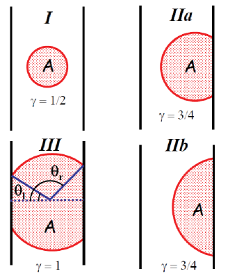
Figure 12: Particular trajectories showing the four different possibilities described in Fig. (10). The spectrum is obtained from quantization of the shaded areas.

The description of a ribbon with two edges is straightforward when the two edges are sufficiently far apart compared to the cyclotron length. Here we consider the situation where this is not necessarily the case, that is when the distance $d>0$ between the two edges is of the order of a few magnetic lengths $\ell_{B}$. The spectrum with two edges obtained numerically for $d=8\ell_{B}$ is shown in Fig. (10), and clearly exhibits three different regions. We now give a full semiclassical description of this spectrum, considering these three different cases. Regions I and II have already been discussed and correspond either to a free cyclotron orbit or to an orbit skipping along one boundary. The new interesting case is the region III for which a cyclotron orbit touches the two boundaries.

We first show that in this case the area $\cal{A}$ to be quantized is the area of a circular orbit cut by the two boundaries (area III in Fig. 12). This may not seem a priori obvious since this area is not bounded by a classical trajectory. Actually a periodic trajectory, the arc $\overset{\;\rotatebox{90.0}{)}}{irf}$ in Fig. 11, encloses an area $\cal{A}^{\prime}$ smaller than ${\cal A}$. Let us return to the argument developed in section (III.A). The Bohr-Sommerfeld quantization rule states that the integral of the velocity along the trajectory $\overset{\;\rotatebox{90.0}{)}}{irf}$ has to be quantized:

$$m\oint_{i}^{f}v_{x}dx=2\pi(n+\gamma)\hbar\ .$$ (27)

$i$ and $f$ are respectively the initial and final points of the periodic trajectory and $r$ is the point where the trajectory bounces on the second boundary (Fig. 11). Now the velocity must be calculated with caution. Along the trajectory $\overset{\;\rotatebox{90.0}{)}}{ir}$, it is given by $v_{x}=-\omega_{c}(y-y_{0})$. Then after the bouncing along the second wall, it is now given by $v_{x}=-\omega_{c}(y+y_{rr^{\prime}}-y_{0})$ where $y_{rr^{\prime}}$ is the distance between the bouncing point $r$ and the point $r^{\prime}$ which is the next intersection between the fictitious cyclotron orbit and the second boundary. Therefore we have:

$${1\over\omega_{c}}\oint v_{x}dx=-\oint_{i}^{f}(y-y_{0})dx-\int_{r}^{f}y_{rr^{\prime}}dx$$ (28)

The first integral on the right side is the area delimited by one period of the motion (${\cal A}^{\prime}$ in Fig. 11) and the second integral is the shaded area (${\cal A}^{\prime\prime}$ in Fig. 11). The sum of these two areas ${\cal A}={\cal A}^{\prime}+{\cal A}^{\prime\prime}$ is indeed the total area delimited by the free cyclotron orbits and the boundaries (Fig. 12.III).

Defining $d>0$ as the distance between the edges, this area ${\cal A}$ is now given by

$${\cal A}(E,x_{c})={R^{2}\over 2}[2\theta_{r}-\sin 2\theta_{r}-2\theta_{l}+\sin 2\theta_{l}]$$ (29)

where $\theta_{r}$ and $\theta_{l}$ define the position of the cyclotron orbits with respect to the two edges (see Fig. 12. We have $\cos\theta_{r}=x_{c}/R$ and $\cos\theta_{l}=(d+x_{c})/R$, where $-d<x_{c}<0$ when the guiding center is inside the sample. The energy levels are semiclassically given by the quantization (12) of the area ${\cal A}(E,x_{c})$ given by (29), where the index $\gamma$ depends on the geometry of the orbit. It is the sum of two terms, $\gamma=\gamma_{l}+\gamma_{r}$, where $\gamma_{l,r}=1/4$ in free space, $\gamma_{l,r}=1/2$ for a skipping orbit, $\gamma_{l,r}=5/12$ when the cyclotron orbit just touches a wall. Between these different values, $\gamma$ varies continuously. In the general case, we have obtained the value of $\gamma(E,x_{c})$ from its decomposition explained above (Eq. 17). Its value is given by

$$\gamma=\gamma_{l}+\gamma_{r}\qquad\mbox{with}\qquad\gamma_{r,l}={1\over 4}\ {1+4e^{AX_{r,l}}\over 1+2e^{AX_{r,l}}}$$ (30)

$$X_{r} = \left({2E\over\hbar\omega_{c}}\right)^{1/6}(x_{c}+\sqrt{2E/\hbar\omega_{c}})$$

$$X_{l} = \left({2E\over\hbar\omega_{c}}\right)^{1/6}(-x_{c}-d+\sqrt{{2E\over\hbar\omega_{c}}})\ .$$ (31)

The function $\gamma(E,x_{c})$ is shown in Fig. 13 as a function of the energy and the position $x_{c}$ in the ribbon. Note that in the limit where the ribbon is narrow $d<<R$, that is in the high energy regime III, we recover straightforwardly that the area is now ${\cal A}(E,x_{c})=2dR$, so that the quantization of this area gives $R=\pi(n+\gamma)\ell_{B}^{2}/d$ and $E_{n}={\hbar^{2}\over 2m}{n^{\prime 2}\pi^{2}\over d^{2}}$, with $n^{\prime}=n+1$, since $\gamma=1$, corresponding to the two reflections on the edges.

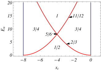
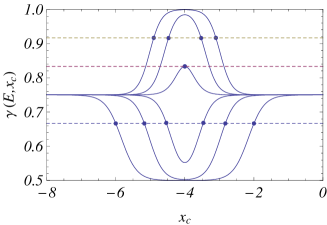
Figure 13: Bottom: dependence $\gamma(E,x_{c})$ versus $x_{c}$ for various fixed energies ($E/\hbar\omega_{c}=2,4,6,8,10,12$, from bottom to top curves). We have indicated the special values ${1\over 2},{2\over 2},{3\over 4},{5\over 6},{11\over 12},1$ corresponding to the different regions shown on the upper diagram.

The spectrum obtained from semiclassical quantization of the area (29) with fixed values of $\gamma=1/2,3/4,1$ corresponding to an free orbit, an orbit touching one or two edges, is displayed in Fig. 14. The approximation is quite good but there are discontinuities corresponding to $x_{c}=-R$ and $x_{c}=-d+R$. In Fig. 15, the spectrum is obtained from quantization of the area, with the appropriate value of $\gamma$ obtained above (Eqs. 30,31). We obtain a perfect quantitative description of the full numerical spectrum.

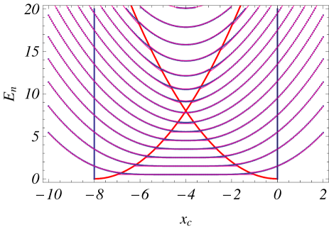
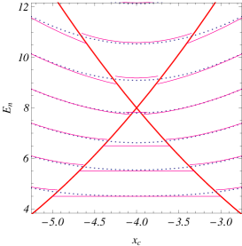
Figure 14: Full curves: Spectrum obtained by semiclassical quantization of the area (29), with fixed values of $\gamma=1/2,3/4,1$ corresponding respectively to free cyclotron orbits, orbits touching one or two edges. Dotted curves: Exact spectrum obtained by numerical calculation. The semiclassical approximation is quite good except when the classical cyclotron orbit approaches the edges. The two parabolas correspond to $x_{c}=-R$ and $x_{c}=-d+R$.

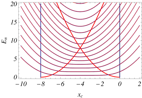
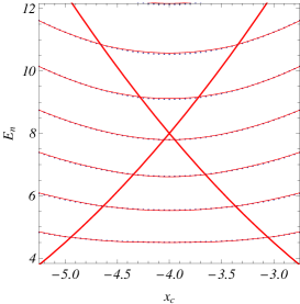
Figure 15: Full curves: Spectrum obtained by semiclassical quantization of the area (29), with $\gamma$ given by Eqs. (30,31). Dotted curves: Exact spectrum obtained by numerical calculation. This semiclassical WKB approximation is now perfect even when the classical cyclotron orbit approaches the edges. The two parabolas correspond to $x_{c}=-R$ and $x_{c}=-d+R$.

V Conclusion

We have provided a semiclassical treatment for the position dependence of the edge states energy levels in the presence of an abrupt infinite potential. This full spectrum may be obtained from the Bohr-Sommerfeld quantization of the area of cyclotron orbits. The orbits do not need to be closed, and the quantization is obtained in all cases, where the orbits hit one or two edges. We provide a simple expression for the mismatch factor $\gamma$ valid for all energies and positions with respect to the boundaries. The situation of an abrupt potential corresponds to a physical limit where the range of variation of the potential at the edge is much smaller than the magnetic length $\ell_{B}$. In the case of a smooth potential, the correct description corresponds to the adiabatic approximation where the energy levels simply follow the potential $V(x_{c})$ at the edge: $E_{n}(x_{c})=(n+1/2)\hbar\omega_{c}+V(x_{c})$, as shown in Fig. 16. An important difference with the case of the abrupt potential is that here the energy profile is exactly the same for all levels. In particular, the drift velocity is $independent$ on $n$ and is simply given by

$$v_{d}={1\over eB}{\partial V\over\partial x_{c}}$$ (32)

and it starts to increase when the potential increases, while for the abrupt potential, the drift velocity depends on $n$, it starts to increase at a distance of order $\sqrt{2n+1}\ell_{B}$ from the boundary (Compare Figs. 4 and 16). Another important difference is that, for an abrupt potential, the maximal value reached by the drift velocity is of order of the Fermi velocity $v_{E}$. If one considers a soft potential of the form $m\omega^{2}(x+x_{0})^{2}/2$, where it is usually assumed that $\omega<\omega_{c}$ (this corresponds to the approximation $\ell_{B}V^{\prime}<\hbar\omega_{c}$), the maximal velocity is of order $v_{E}\omega^{2}/\omega_{c}^{2}$, much smaller than $v_{E}$.

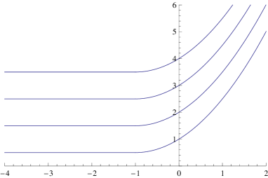
Figure 16: Energy levels in the case of a smooth confining potential $V(x)$. In this case, the energy levels following simply the potential profile: $E_{n}(x_{c})=(n+1/2)\hbar\omega_{c}+V(x_{c})$, compare with Fig. 4.

In conclusion, we have shown that the semiclassical picture of quantized skipping orbits leads to a quantitative description of the edge states energy spectrum. We believe that this quite simple description, not only has a pedagogical interest, but may allow the study of physical quantities not very much discussed in the literature, like the drift velocity. We believe also that it can help for the description of more sophisticated problem like the structure of edge states in graphene.BreyFertig ; Delplace

- (1) B. I. Halperin, Phys. Rev. B 25, 2185 (1982).
- (2) A. H. Macdonald and P. Streda, Phys. Rev. B29, 1616 (1984).
- (3) M. Büttiker, Phys. Rev. B 38, 9375 (1988).
- (4) M. Büttiker, in Nanostructured systems, M. Reed ed., Semiconductors and semimetals, 35, 191 (Academic Press, Boston, 1991); C. L. Kane and M. P. A. Fisher, in Perspectives in Quantum Hall Effects, p.109 (Wiley Interscience 2007)
- (5) H. Van Houten, C.W.J. Beenakker, J.G. Williamson, M.E. Broekaart, P.H.M. Loosdrecht, B.J. van Wees, J.E. Mooij, C.T. Foxon and J.J Harris, Phys. Rev. B 39, 8556 (1989); H. Van Houten and C.W.J. Beenakker, in Analogies in Optics and Micro Electronics, W. Van Haeringen and P. Lenstra eds. (Kluwer, Dordrecht, 1990)
- (6) L. Brey and H. A. Fertig, Phys. Rev. B 73, 235411 (2006)
- (7) P. Delplace and G. Montambaux, in preparation
- (8) See for example H. Friedrich and J. Trost, Phys. Rev. A, 54 (1996). The Maslov indices are usually defined such as
- (9) Y. Avishai and G. Montambaux, Eur. Phys. J. B, 66, 41 (2008)
- (10) In ref. Avishai08 , the action was defined along half a period.