Superconductor-Insulator transition and energy localization
Abstract
We develop an analytical theory for generic disorder-driven quantum phase transitions. We apply this formalism to the superconductor-insulator transition and we briefly discuss the applications to the order-disorder transition in quantum magnets. The effective spin- models for these transitions are solved in the cavity approximation which becomes exact on a Bethe lattice with large branching number and weak dimensionless coupling . The characteristic features of the low temperature phase is a large self-formed inhomogeneity of the order-parameter distribution near the critical point where the critical temperature of the ordering transition vanishes. We find that the local probability distribution of the order parameter has a long power-law tail in the region where is much larger than its typical value . Near the quantum critical point, at , the typical value of the order parameter vanishes exponentially, while the spatial scale of the order parameter inhomogeneities diverges as . In the disordered regime, realized at we find actually two distinct phases characterized by different behavior of relaxation rates. The first phase exists in an intermediate range of . It has two regimes of energies: at low excitation energies, , the many-body spectrum of the model is discrete, with zero level widths, while at the level acquire a non-zero width which is self-generated by the many-body interactions. In this phase the spin model provides by itself an intrinsic thermal bath. Another phase is obtained at smaller , where all the eigenstates are discrete, corresponding to full many-body localization. These results provide an explanation for the activated behavior of the resistivity in amorphous materials on the insulating side near the SI transition and a semi-quantitative description of the scanning tunneling data on its superconductive side.
pacs:
03.67I Introduction
Recently the subject of zero temperature quantum phase transitions and of the corresponding quantum critical points in translationally invariant systems got a lot of attention, the theoretical description of this phenomenon is mostly complete.Sachdev2000 Much less is known and understood about the transition driven by the competition of a strong disorder and interactions in quantum systems which is the subject of this paper.
The goal of the paper is twofold: to formulate a theoretical model that is relevant for the description of a number of experimental systems and to solve this model in the simplest controlled approximation. The physical systems that we shall focus on are disordered superconductors but the main results can also be applicable to disordered magnets, especially disordered ferromagnets in a random field. The new physics introduced by the strong disorder is the appearance of new phases Basko2006 in which all or some excitations are localized in space and have infinite lifetime and thus cannot contribute to any transport. The quantum critical point at which the long range order appears has many features that distinguish it from a conventional quantum critical point in a translationally invariant systems, most notably it is characterized by a wide distribution of the order parameter in a realistic system and the appearance of a new intermediate phase in which only low energy local excitations have infinitely long lifetime while high energy excitations can decay.
In Section II we analyze the experimental data on superconductor-insulator (SI) transitions in disordered films of InO, TiN and Be and argue that this transition is driven by the competition of disorder and superconductivity with very little effect of the Coulomb repulsion. This will allow us to formulate a theoretical model for this quantum transition which is nothing but the model introduced in a seminal work by Ma and Lee MaLee1985 . In Section III we develop the formalism to study the formation of the order parameter in this model at zero temperatures. In this formalism the appearance of a wide distribution of the order parameter shows up as replica symmetry breaking. Our theory provides the justification for the qualitative idea of the importance of rare sites characterized by a very large susceptibility, an idea that was first suggested by by Ma, Halperin and Lee MaHalperinLee and observed in the solution of similar one-dimensional models MaDasgupta ; Fisher1992 . In Section IV we study the properties of the insulating state. We first determine the level width (decay rate) at zero temperature and then extend the analysis to low temperatures. We find two phases in the resulting insulator: an intermediate phase where only excitations of large enough energy can decay and a third phase, in the strong disorder regime, characterized by the infinite lifetime of all excitations, similar to the one proposed in Basko2006 . In Section V we discuss the effect of a magnetic field on the phase diagram within our model of the SI transition. The main conclusion of this Section is that the effects of the frustration induced by magnetic field are small; this can be understood as a consequence of the strong inhomogeneity of the order parameter in the vicinity of the transition. In Section VI we discuss the direct implications of the theory for the experiments and propose numerical simulations that should test the applicability of the theory to realistic models. Section VII gives conclusions.
A first quantitative study of the phase diagram of the Ma-Lee model has appeared recently in IoffeMezard2010 . The present paper provides a much more detailed derivation, and studies in detail the behavior of the order parameter and level width. Similar qualitative conclusions on the reelvance of the Ma-Lee model and the phase diagram were reached from phenomenological considerations in the recent paper Muller2009 .
II Superconductor-insulator transition: data and the model.
II.1 Experimental results
We begin with the analysis of the data on strongly disordered superconducting films. Our goal is to formulate the simplest model that captures the essential physics of these systems. Strongly disordered films of InO, TiN or Be display a zero field transition from superconductor to insulator when their resistivity in normal state exceeds a value of the order of the resistance quantum . SITReview ; Gantm2010 The films in the superconducting state close to the transition become insulating when subject to a magnetic field.Hebard1990 ; Shahar2004 ; Kapitulnik2008 The transition driven by magnetic field display a quantum critical point behavior: the resistance of the films at fields decreases with temperature decrease while the resistance of the films at increases with temperature decrease. Very important information is provided by tunneling spectroscopy of such superconducting films in the vicinity of the quantum critical pointSacepe2007 ; Sacepe2008 ; Sacepe2009 ; Sacepe2010 . These data show a well defined gap at all points whilst the coherence peaks expected for a BCS superconductor appear at some locations and do not appear at others; a similar phenomenon was reported for high oxidesKapitulnik2001 ; Davis2001 ; Davis2002 ; Yazdani2007 . The absence of coherence peaks combined with intact superconducting gap in a single electron tunneling experiment implies that the disorder does not destroy local Cooper pairing of electrons but prevents formation of the coherent state of these pairs. This allows to exclude a fermionic mechanism of superconductivity suppression in these materials: in such an alternative scenario, the main role of the disorder would be to enhance the Coulomb interaction that competes with phonon attraction. This would lead to the suppression of the transition temperature and the superconducting gap and to the eventual disappearance of both the superconductivity and the gap. In contrast, the InO and TiN data demonstrate the presence of a large one-particle gap in the absence of global coherence and a smooth crossover between superconducting and insulating gaps as disorder is increased (see Feigelman2010 for more detailed discussion).
In the absence of single-electron excitations, the supercondutor-insulator (SI) transition might happen either because the Coulomb interaction between the pairs prevents the formation of the condensate, or because the disorder of Cooper-pair energies prevents their coherent motion from one site to another. The first scenario might be realized in the granular materials in which superconductivity remains basically intact in each grain. The grains are coupled to each other by Josephson couplings which compete with the Coulomb energy that changes when a pair moves from one grain to another. Exactly the same physics is realized in Josephson junction arrays which were extensively studied some years ago.vanderZant1996 ; Fazio2001 ; Serret2002 In particular, it was established that in the presence of a magnetic field the Josephson arrays display a temperature-independent resistance that varies by many orders of magnitude as a function of a weak magnetic field. In other words, in these arrays the SI transition does not happen directly, instead there is a wide region of intermediate ’normal’ phase. This behavior is very surprising given the absence of single electron excitations in these arrays. It is probably due to the formation of a Cooper-pairs glass, similar to the electron glass; in this regime collective modes provide the dissipation mechanism. Although the theoretical picture of this phase is not clear, the observed experimental behavior of these systems is in a striking contrast with the behavior of disordered films which show a direct transition between superconductor and insulator.
This leaves the only possible mechanism for the superconductor-insulator transition in disordered films: the competition between pair hopping and random pair energies on different sites, as suggested 25 years ago in a seminal paper of Ma and Lee MaLee1985 (see also BulSad ; KotKap ; Randeria ). As we show in the present paper, the solution of this model reproduces correctly the most important features of the data: direct SI transition, activated behavior close to the quantum critical point in the insulating phase, strong dependence of the activation energy near the quantum critical point and huge order parameter variations from site to site in the superconducting phase.
Recent experimental data indicate the possibility of a faster than activated temperature dependence of the resistance in the insulating phase (characterized by growing at low ). This behavior is very unusual for disordered electron systems which typically display either activated, Efros-Shklovskii or Mott behavior characterized by with . It can be understood if the pair excitations remain localized in space at low energies but are delocalized at high energies with the temperature dependent mobility edge that separates them.
For the microscopic justification of this mechanism one needs to find the reason why Coulomb repulsion does not play a role in the superconductor - insulator transition in some disordered films. Phenomenologically, it is known Zvi that the dielectric constant in these materials remains very large, deep in the insulating phase of InOx. A large value of the dielectric constant between low energy electrons close to the Fermi surface allows one to neglect the effect of Coulomb interaction on the pairing even for relatively strong disorder that results in wave functions localization. Because the host matrix dielectric constant can only increase with additional carriers, the Coulomb interaction between conducting electrons close to the Fermi surface is strongly suppressed in this materials. The microscopic reason for that might be a very strong energy dependence of the density of states (in particular, it was computed for a typical small cluster of TiNAnisimov ), this implies that although density of states exactly at the Fermi level is small and the states there get localized, there are many single electron states within range that provide large screening of the bare Coulomb interaction.
A detailed analysis of the competition between Cooper pairing and wave-function localization is provided by a recent paperFeigelman2010 . In particular, it shows that global superconductivity can survive in a range of relatively strong disorder. Within this scenario the localized electron pairs are formed at high temperatures when two electrons bind together (with typical binding energy ) on a weakly localized state. At lower temperatures, , coherent hopping of these pairs leads to the long-range coherence and to the formation of a superconducting condensate. Direct experimental confirmation of this scenario is provided by the scanning tunneling microscopy dataSacepe2007 ; Sacepe2008 ; Sacepe2009 ; Sacepe2010 . At even stronger disorder long-range coherence is never formed, the resulting state is insulating, characterized by a large single-particle gap.
The paper Feigelman2010 studied the properties of the superconducting and insulating phases far from the transition. In this work we study the properties of these phases in the vicinity of the transition in which the characteristic energy scales are much smaller than the single particle gap, . In this study we shall focus on these low energy scales and neglect the contribution from single-electron occupied localized orbitals. This allows us to describe the physics entirely in terms of Anderson pseudospins Anderson1959 . The interaction between the pseudospins is due to the matrix elements of the Cooper attraction between original electrons. As discussed in the work Feigelman2010 these matrix elements are modified by the fractal nature of the electron wave functions which leads to correlations and to a smooth dependence of on disorder strength. In the present paper we shall ignore the effect of fractality that should not affect the qualitative properties in the vicinity of SI transition. In the absence of such correlations the average interaction between pseudospins does not depend on disorder. Thus, when comparing with experimental data we shall assume that changing of the disorder translates only into changing the number of "interacting neighbours" of a given pseudospin.
II.2 The model: localized pairs and pseudospin representation.
In the absence of Coulomb repulsion the only interaction between electrons is the attraction that leads to their pairing on the localized single electron states.Feigelman2010 The strength of this pairing is inversely proportional to the volume of the state. Because of the fractal nature of the single electron wave functions the volume of a typical localized state is small, this makes the pairing energy large. Thus, the low energy degrees of freedom in this system are pairs that can hop from one site to another. This physics is described by a Hamiltonian of disordered hard-core bosons, or, equivalently, pseudospin operators (originally introduced by AndersonAnderson1959 for the pure system, and later by Ma and LeeMaLee1985 for the disordered system):
| (1) |
where are spin- operators and the sum goes over all different pairs of neighbors . The state with corresponds to a local level occupied or unoccupied by a Cooper pair; ’s are occupation energies for each site, which are quenched random variables drawn from a probability distribution . Hereafter we assume a box distribution , so that the non-interacting density of states is . The important feature of this distribution is that it is constant near to ; the value of just sets the scale of energies, and we shall choose . The matrix elements describe the hopping amplitudes of Cooper pairs. These hopping amplitudes couple a typical local level to a large number of neighbors, . We shall assume that each site is coupled to neighbors with . Another closely related problem corresponds to the Ising ferromagnet in a random transverse field; the model is defined by the Hamiltonian
| (2) |
For brevity we shall refer to this model as Ising model below. We shall mainly study the XY problem (1) but most of our conclusions also hold for the case (2). As will be clear below, in the leading approximation the two models (1) and (2) lead to identical cavity equations for both the order parameter and the relaxation rate.
The Hamiltonian (1) describes the superconductor-insulating transition as a ferromagnetic spin system with random transverse fields, as proposed originally inAnderson1959 ; MaLee1985 . In this language the superconducting phase corresponds to the existence of a spontaneous magnetization in the plane.
III Formation of a long-range superconducting order.
III.1 A simple mean-field approach
The most obvious approach to study the Hamiltonians (1,2) is to use the mean-field approach, in which is replaced by where is determined self-consistently from the equation . The right-hand side of this equation contains a sum of terms, so it might be expected to become site-independent in the large limit. Although we shall challenge below the assumptions and conclusions of this approach, it is instructive to summarize its main results. The mean field Hamiltonian on site has two eigenstates with energies where . At temperature , one obtains the self consistent equation for , which gives either or
| (3) |
At zero temperature this equation has a solution for any , so the ground state is characterized by a non-zero field, . This corresponds to a spontaneous order parameter (in spin language, this is a non-zero magnetization) in the direction, so the system is a superconductor (or a ferromagnet in case of the Ising model). At finite temperature there is a transition from an insulating to a superconducting phase, when (3) starts to have a solution. Assuming a constant density of states, , we find that the critical temperature is determined by:
| (4) |
where is the Euler number. As we show below, while this mean field prediction is correct at , it is qualitatively wrong for a system with a finite connectivity (even if is large) in the limit of very small .
III.2 Cavity mapping
We now turn to a more refined mean-field discussion, valid for finite , which is the basis for our main results. We shall employ the cavity method that has been developed in the classical case to study frustrated systems on a Bethe lattice, a fixed connectivity random graph of connectivity , see MezardParisi2001 . Its generalization to quantum problems without disorder has been studied in Laumann ; Krzakala , using the Suzuki-Trotter formalism. We shall use here an approximation of the quantum cavity method which does not use the Suzuki-Trotter formalism, and allows to study analytically the quantum disordered systems. As we shall see below (see discussion below (21) and section III.7), this method takes into account the leading corrections to the naive mean field at large-but-finite , which turn out to be of order . It neglects the corrections that are small in . Appendix A explains the relation of our approach to the full Suzuki-Trotter quantum cavity method.
In the simplified cavity method one emulates the effects of spin environment by the static field acting on it. One thus studies the properties of a spin in the cavity graph where one of its neighbors has been deleted, assuming that the remaining neighbors are uncorrelated. The system of spin and its neighbors is thus described by the local Hamiltonian
| (5) |
where is the local “cavity” field on spin due to the rest of the spins (in absence of ). Here we have chosen the direction as the transverse direction where the spontaneous ordering takes place. By solving the problem of spins in (5), one can compute the induced magnetization of , , which is by definition equal to . One thus gets a mapping allowing to compute the new cavity field in terms of the fields on the neighboring spins. This mapping induces a self-consistent equation for the distribution of the fields MezardParisi2001 . Notice that the use of the mean-field approximation in order to study the cavity mapping is very different from its naive use in (2).
One can make one more approximation which simplifies the cavity mapping and makes possible an analytical study. Similarly to the mean-field approach discussed above, one can replace dynamical spin variables by their averages. This approximation neglects some terms of order of ; below we refer to it as the cavity-mean-field approximation. We shall first study this approximation here. Later on, in section III.7, we shall compare its results with the ones found by the full cavity mapping. As we show in this section the cavity-mean-field approximation becomes very accurate even for moderately small . The physical reason for this is that the main effect missed by the cavity-mean-field approximation is the level repulsion induced by the interaction between sites and . However this repulsion happens only in the rare cases when is close to , and it has a significant effect on the resulting value of the local order parameter only when both of them are close to . Because this happens very rarely, the cavity-mean-field approximation turns out to be very good for this problem.
Formally, the cavity mean field approximation amounts to approximating the cavity Hamiltonian (5) acting on spin by
| (6) |
This implies that , giving the recursion equation relating the fields:
| (7) |
This recursion induces a self-consistent equation for the distribution :
| (8) |
This equation always allows the trivial solution corresponding to an insulator. The superconducting transition is signaled by the appearance of another solution characterized by a non-trivial distribution function . It turns out that this transition and the properties of the phases in its vicinity can be best studied using methods developed in the statistical physics of random systems.
III.3 The directed polymer problem and replica symmetry breaking
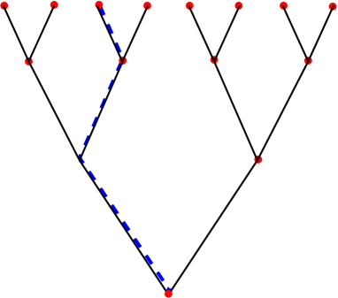
In order to understand the properties of the mapping (7), let us imagine that we iterate it times on a Bethe lattice. For finite and the corresponding graph is just a rooted tree with branching factor at each node and depth (see Fig. 1). The field at the root is a function of the fields on the boundary. In order to see whether there is spontaneous ordering, we study the value of in linear response to infinitesimal fields on the boundary spins. This is given by
| (9) |
where the sum is over all paths going from the root to the boundary, and the product is over all edges along the path . The response is nothing but the partition function for a directed polymer (DP) on a tree, where the energy of each edge is and the temperature has been set equal to one. The general method for the solution of such problems has been developed by Derrida and SpohnDerrSpohn . The solution can be expressed in terms of the convex function
| (10) |
Let us denote by the value of where this function is minimal. In the large limit, there exist two regimes for the DP problem:
-
•
“RS-phase”: If , then . In this case the superconducting phase appears at a value which is the same result as found by the naive mean field approach in (4).
-
•
“RSB-phase”: If , then . The ordered phase appears at which is larger than the naive estimate (4).
The method for obtaining these results developed by Derrida and SpohnDerrSpohn employed a mapping to the traveling wave equations. An alternative way, which we now summarize, is to use the replica method, similar to the one used inCookDerrida90 . It gives a compact solution and helps to understand the physical meaning of the DP phase transition. The names of the two phases used above (“RS” stands for replica symmetric” and “RSB” stands for replica-symmetry broken”) originate from this analysis.
The DP partition function , defined in (9), depends on the random quenched variables . One expects that the free-energy in a short-range-interaction problem is a self-averaging quantity, so the value of for a typical sample is obtained from the quenched average of over these random variables, denoted by . In the replica method one computes it by writing
| (11) |
The average of is obtained by a sum over paths,
| (12) |
where the weight of each edge in the tree depends on the number of paths which go through this edge.
The RS solution assumes that the leading contribution to (12) comes from non-overlapping independent paths (). This gives
| (13) |
The RSB solution assumes that the leading contribution to (12) comes from patterns of paths which consist of groups of identical paths, where the various groups go through distinct edges. This gives:
| (14) |
where is the function introduced in (10). In the replica limit , the parameter should belong to the interval . Minimizing the function over (the fact that one should minimize , and not maximize it, is a well-known aspect of the replica method MezardParisiVirasoro ), one gets the phase diagram described above: there exists a critical value of the inverse temperature such that, for , the function is minimal at the boundary, of the interval ; the DP is in its replica symmetric phase. For , the function has a minimum inside the interval at some value , this corresponds to the spontaneous breakdown of the replica symmetry in the DP problem.
These two regimes of the DP problem are qualitatively very different. In the RS regime the measure on paths defined in (9) is more or less evenly distributed among all paths. On the contrary, the RSB regime is a glass phase where the measure condenses onto a small number of paths. An order parameter which distinguishes between these two phases is the participation ratio , where is the relative weight of path in the measure (9). It is easy to see that in the RS phase. In the RSB phase, the value of is finite and non self-averaging (it depends on the realization of the ’s), and its average is given by . This glass transition, and the nature of the RSB glass phase, are identical to the ones found in the random energy model DerridaREM ; GrossMezard .
III.4 Phase diagram
The results on the DP problem described in the previous section allow to derive the phase diagram of disordered superconductors. The state of the model is determined by the three parameters: the coupling , the cavity connectivity , and the temperature . The phase transition between insulator and superconductor is a surface in this three-dimensional parameter space. Depending on the purpose, it can be useful to view it in different directions. We shall define the phase transition as , or , or . In the zero-temperature limit we shall speak of and .
The DP partition function gives the susceptibility, measured on the root site, to a small field on the boundary. When this susceptibility diverges, there is spontaneous generation of non-zero fields, i.e. the systems is in the superconducting phase. The superconducting phase transition point is given by:
-
•
If (RS phase of the DP), then . This coincides with the result of the naive mean field analysis.
-
•
If (RSB phase of the DP), the phase transition is obtained by solving the two equations and .
At zero temperature the function can be computed analytically:
| (15) |
leading to two equations for and which have the explicit solution
| (16) | |||||
| (17) |
The value of determined by the solution of (16) gives the location of the zero temperature quantum phase transition between the insulating and the superconducting phase. Note that in the framework of the recursion equations (7) this is an exact result. It predicts a finite value of for all . In particular, when it reproduces correctly the result known for the one-dimensional chain Fisher1992 . This is in contrast with the naive mean field equation (4) which wrongly predicts for all . For the comparison with the experiment it will be useful to describe the phase transition point as a function of the effective number of cavity neighbors for a given a value of the hopping (see section II.1); in terms of this parameter the system becomes superconducting at . The zero temperature transition point is given by explicit equation:
| (18) |
We now discuss the finite temperature phase transition. At sufficiently high temperatures, , the transition line is independent of and is given by the naive mean field result (4): . The RSB solution appears at a value such that . At this the derivative , which gives two equations that determine the position of this point on or plane:
| (19) | |||||
| (20) |
The result is again best expressed by inverting in order to get the critical value below which the naive mean field solution breaks down. The asymptotic of the solution of the equations at is
| (21) |
The equations for the critical values of the number of neighbors (18,21) show that, at large , the solution deviates from the naive mean field solution of section III.1 at . This demonstrates that our approximation takes into account corrections, as announced above. Note that at weak coupling is exponentially larger than , so that there is a broad range of where RSB effects are important.
An important unexpected qualitative conclusion from (21) is that the effective number of neighbors of a given site, , defined as the number of neighbors having local energies within the energy stripe , is typically much smaller than unity. Indeed, at the temperature , this number is given by
| (22) |
it decreases with roughly as when . Although is small, it leads to a non-zero and to RSB effects. This is another signature of the fact that the transition is governed by rare sites.
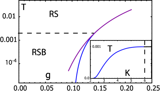
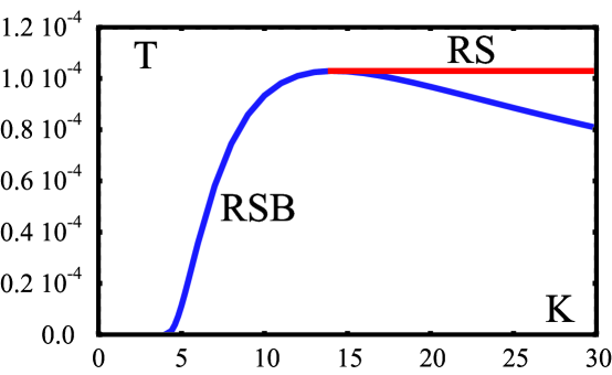
The phase diagram for is shown in Fig. 2. At any temperature, there is a finite critical value of the coupling, , separating an “ordered”, superconducting, phase with spontaneous order parameter at from a “disordered” normal phase with zero order parameter at . Contrary to the naive MF prediction, remains non-zero at .
One of the important characteristic properties of the quantum critical point is the behavior of near to the critical point where it drops to zero. In order to study this behavior, we look for the solution of the two equations and . The explicit form of these equations is
| (23) | |||||
| (24) |
We assume that with , and we introduce the quantity , which is expected to be close to its critical value . The second equation (24) leads to the relation . Next, in order to determine we use the stationarity of the first equation with respect to the simultaneous variations of , and , and find
| (25) |
with
The result (25) is valid as long as is much less than the mean-field transition temperature and . In terms of the former condition is
| (26) |
For physically relevant systems , so the condition (26) determines the regime of for which the result (25) holds. This analysis shows that the transition temperature goes down very slowly when decrease below the value, until it reaches the close vicinity of where it drops sharply to zero according to Eq.(25). The numerical solution of Eqs.(23,24) for at is presented in Fig.2 (insert).
The replica symmetry breaking at , which is at the origin of the failure of the naive mean field analysis, has important physical consequences. Physically it signifies the absence of self averaging which is due to the importance of very rare sites with small that easily polarize in the -direction, becoming thus nucleation centers for the ordered phase. The qualitative importance of these rare sites and resulting absence of self averaging was first discussed in MaHalperinLee . Our analysis gives the mathematical formalism to evaluate these effects and their consequences within the well-controlled Bethe approximation, such as the exact position of the phase transition point. The role of rare sites with small can be quantitatively characterized by the condensation of the measure in the DP problem. Let us imagine adding a small field in the direction on one site , and let us look at its effect on the spins at distance from ; this gives the picture of the correlations in the many-body wave-function. In the RSB phase, the order develops only along a small number of paths; this fact is completely missed by the naive mean field approach.
Even at the self averaging is not fully restored. In particular, in a wide range of the simple mean-field approximation is not applicable for the calculation of higher moments of the distribution. The upper border of this region is given by the value corresponding to the divergence of infinitely high moments (divergence of at ). The condition for this divergence is given by the inequality . With determined by the mean-field approximation, we get the critical value that corresponds to the divergence of large moments:
| (27) |
where is the Euler number. The full self-averaging is expected only at .
III.5 Distribution function of the local order parameters and the phase diagram.
In this section we derive the equation for the distribution function of local fields close to the transition point, , using the cavity mapping (7) as the starting point. We will use the Laplace transform of this distribution, .
We start from the linearized version of Eq.(7),
| (28) |
which is adequate to describe the phase transition region where the fields are small. The Laplace transform satisfies the equation:
| (29) |
Consider the first terms of its expansion at small , and assume that this expansion behaves as . If , the mean is finite. We will see that this is the situation in the RS phase. The situation occurs in the RSB phase, and corresponds to a distribution which decays at large like , with a diverging mean.
Let us first assume that . Then is just the mean of , i.e. it coincides with the usual superconducting order parameter. Plugging into (29), the resolvability condition for the linear equation in leads immediately to the standard mean-field equation for , see (4). We learned previously from the replica analysis that this equation is valid only in the RS regime: it is not correct when . Therefore, RSB corresponds to the divergence of the mean order parameter. To study the RSB phase, we assume that with . From (29), we obtain the condition
| (30) |
which can also be written by using the function introduced in the replica analysis as . Therefore, for any , there is a non-trivial solution . In this situation, it is reasonable to assume that the critical value of is the largest one among all these values, which means that it is obtained by finding the minimum of . We shall prove this assumption in section III.9 where we study the spatial evolution of the distribution function. This is precisely the result obtained with the replica solution in section III.4 of the DP problem, with defined in Eq.(17), a solution which coincides with the result obtained by travelling waves analysis DerrSpohn when applied to this problem. The corresponding distribution function is characterized by a power-law behavior at large , where is of the order of a typical value of :
| (31) |
This power-law tail at large translates into the behavior of the Laplace transform:
| (32) |
III.6 Scaling of the order parameter close to the transition
The expansion of the mean field equation (3) would give an order parameter which scales as close to the transition. This is the usual mean-field scaling. It is modified by the strong fluctuations of local ordering fields present in our problem. As we discuss in section III.6.1 this modification is present even in the some range of parameters in replica symmetric phase not too far from RSB transition and, of course, in the whole low temperature regime where RSB happens. We shall analyze these two cases successively.
III.6.1 Replica symmetric regime at large .
The nonlinear recursion relation (7) leads to the equation for the average value
| (33) |
At , or defined in Eq.(21), the transition temperature is determined by Eq.(4). We assume now that, just below the transition line , the distribution has a scaling form , with vanishing at .
We begin by repeating the usual mean field arguments. Assuming that decays faster than , so that the integral , we can expand
We use the equation (4) for the critical point to reduce (33) to the form
| (34) |
which leads to the usual mean-field scaling .
Clearly, the crucial assumption used in this solution is that the third moment of (i.e. ) is finite. It breaks down if decays at large like with . Notice that in this regime the mean value of is finite, therefore it belongs to the replica symmetric phase from the point of view of the equations giving the critical temperature discussed in section III.4. The behavior of at large can be studied by the Laplace transform method developed in section III.5. More precisely, we assume that the Laplace transform at small has a form with , insert it in the general recursion equation (29) and solve the resulting equations for the coefficient and the exponent . The computation shows that the exponent is the solution of the equation . The mean field scaling holds if and only if this solution satisfies . This happens when
| (35) |
The result for Laplace transform implies that in the regime the distribution on the critical line decays as with and . In this case the equation (34) for the order parameter is replaced by
| (36) |
This implies the anomalous scaling of the order parameter near the critical line:
| (37) |
Note that when the exponent so that dependence reduces to the usual square-root singularity. At the opposite end of the interval , the exponent in Eq.(37) diverges because as .
III.6.2 Regime of broken replica symmetry.
The RSB transition affects dramatically the scaling of the field in the ordered phase in the vicinity of the transition. As we have seen in subsection III.6.1, in order to derive this scaling we need to know the distribution of fields induced by the mapping (7). As discussed in section III.5 the expansion of its Laplace transform shows that exactly on the transition line , in the RSB regime, the distribution function decays at large as . Here is the RSB parameter identified in our analysis of the directed polymer problem as the value of where is minimal.
For larger than but close to the transition, a small typical field, , appears. At the usual scaling arguments show that the distribution retains the same scaling form (31) that it acquired at . As we show below this scaling law is cut off from above by , beyond which decays rapidly. The power law behavior of in a wide range of fields allows one to find analytically the typical field from the following reasoning. Because the integral is logarithmic, the main contribution to the expectation value of comes equally from a very broad range of fields . Because of this wide range of fields contributing to the expectation value, the ’th power of (7) is dominated by the largest term in the sum, so that
| (38) |
Similar arguments of dominance of the largest term justify the cutoff at . Because each term in the sum (7) is cut off by and the sum is dominated by the largest term, the power-law behavior (31) is effectively cut off by , while at it decreases exponentially.
Averaging the approximate mapping for (38) we get the equation:
| (39) |
To proceed further we write the equation for the transition line, , in the form similar to Eq.(39):
| (40) |
| (41) |
As will be clear below, the qualitative properties of the solution are the same at zero and finite temperatures. So, to simplify the formulas we focus on the vicinity of the zero-temperature quantum critical point , . In this regime we can replace all functions by 1 and get
| (42) |
where
| (43) |
In the large regime which is of main interest to us, , and . Using our Ansatz for the distribution function, valid in the broad range of , we find:
| (44) |
Here, and in the following, denotes a numerical constant of order 1. Using the estimate for discussed above we get
| (45) |
For we expand the exponent in Eq.(45) and find
| (46) |
This gives the typical value of the order parameter close to the transition; in contrast to quantum critical points in clean systems the behavior displays an essential singularity. This result becomes even more surprising when one compares to the critical temperature (which follows from Eq.(25)) because it implies that the typical order parameter at is much smaller than the transition temperature at the same value of .
Eq. (45) gives the dependence of the order parameter as a function of the interaction constant at very low temperatures for close to . Similar arguments give the dependence of the order parameter at as function of temperature in the vicinity of transition:
| (47) |
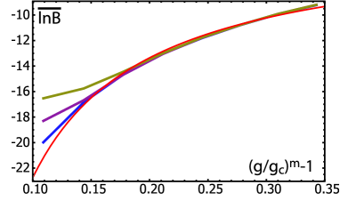
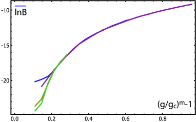
Because this analytical derivation relies on our Ansatz for the distribution function, we have checked the scaling behavior (45) numerically. We solve the self consistent equation (8) for using the population dynamics algorithm developed in work MezardParisi2001 . In a nutshell, this method amounts to approximating by a population of fields, which is sampled by a Monte Carlo method iterating Eq.(7). In order to tame the effects of rare fluctuations, it is numerically convenient to put the system in a small external field, using the mapping (48) defined below in the Section III.8. The results are reliable (as can be checked from the fact that they do not depend on the external field at small enough field) when is not too close to . The results for (for which the zero-temperature critical coupling is and ) are shown in Fig. 3 where we plotted as a function of for and its fit to a dependence: with , . This value of is close to the one expected from (45) because for this value of one has .
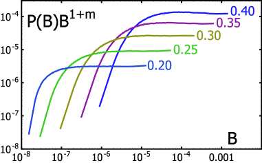
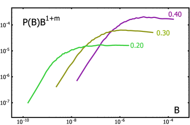
The computations above are based on the assumption that the distribution function retains its power-law dependence in the ordered phase in a wide range of fields. We have checked this assumption directly using population dynamics. The result is shown in Fig. 4. One observes that develops a plateau that becomes wider on a logarithmic scale when one approaches the quantum critical point.
III.7 Leading correction in to the RSB solution.
As we explained in section III.2, the full cavity Hamiltonian (5) can be approximately replaced by the simpler Hamiltonian (6) in which the dynamics variables were replaced by their averages . This approximation ignores dynamic quantum correlations between the spin at site and its neighbors at site . These correlations might become important when the energies of these two sites are close, so that . Such resonance conditions occur with a probability which is small at large . To check that these and other corrections are not relevant at modest values of we have performed a population dynamics simulation of the full cavity mapping (5). At each step of this simulation we start with the population of spins characterized by energies and fields We randomly choose sets of spins from this population, add to each of them an additional spin with random energy and diagonalize the corresponding Hamiltonian (5) to determine the effective value of the field acting on the additional spin. This gives a new set of spins with energies and fields A typical simulation involved spins and steps which is sufficient to get the convergence of the typical field at .
In Fig. 5 we compare the results of the full diagonalization with the simplified mapping for As one can see from these results, even at these modest value of the results of the full cavity mapping are indistinguishable from the simplified mapping. Qualitatively it means that the important physics driving this transition is the appearance of wide distribution of fields, and this effect is not sensitive to quantum correlations neglected by the simplified mapping.
III.8 Susceptibility in the disordered phase.
We now study the approach to the quantum critical point coming from the insulating phase. In usual phase transitions the order parameter induced by a small external field diverges at the transition, corresponding to a divergent linear susceptibility. We shall see that the situation is very different here: there is no diverging susceptibility.
We focus on the insulating phase at and . We apply a very small uniform external field to all sites. Repeating the same arguments as before we arrive at the cavity-mean-field mapping
| (48) |
For very small , in linear response, the induced fields are also small. We can thus neglect the non-linearity in this equation at . In the resulting linear equation we can rescale the variables and get
| (49) |
All properties of the solution are contained in the distribution function generated by the mapping (49). In order to study this function, it is convenient to introduce the Laplace transform . It satisfies a self-consistent equation that can be derived directly from the mapping (49):
| (50) |
We assume the existence of and derive some of its properties. The behavior at small is easily found: if we look for a solution in the form , we get the equation for the exponent :
This equation is equivalent to the equation for the RSB parameter at , see Eq.(16). Therefore .
When we look for a solution in the form . Inserting it into the equation (50) we get, for :
| (51) |
In order to prove the existence and stability of this solution we solved the equation (50) numerically. In order to check the analytical asymptotic we need to have the solution in a broad range of parameter . For this reason we have transformed the equation (50) by introducing the variables , :
| (52) |
and solved the resulting equation by iteration for and . The result is displayed in Fig. 6. The low asymptotic is indeed , with the correct value of . The asymptotic behavior at large is more tricky because the exponential dependence with parameters given in Eq.(51) is expected to occur when ; this condition implies that in this regime which is difficult to access numerically. In the transient regime of the numerical solution fits exponential dependence with somewhat different parameters, and .
The existence of a stable solution of the equation (50) implies a number of unusual properties of this quantum phase transition. A small external field induces some non-zero fields . Let us compute the average . It can be expressed through the Laplace transform by
The behavior implies that for the average . In particular, the typical induced order parameter is of the order of the external applied field: . But the moments with , and in particular the mean , are divergent at the level of the linear response to . The non-linearity of the mapping neglected in (49) cuts off this divergence at . One can therefore expect a non-linear response when . These results show that the response to an external field, computed at , has no singularity at the transition. This behavior is totally different from the one in usual phase transitions. We illustrate this by Fig. 7 which shows the average and typical fields induced by a small external field at .
III.9 Spatial scale of inhomogeneities of the order parameter.
Close to the transition the spatial scales beyond which the system is uniform become very large. In particular, at temperatures below that of replica symmetry breaking, the susceptibility is dominated by a single path, as discussed above, in Section III.3, implying that the system is essentially non-uniform at all length scales. The goal of this section is to compute the characteristic scales at which the system becomes uniform in the ordered state.
The non-uniformity at short scales is related to the fact that close to the transition the order parameter in the infinite system is power-law distributed in an exponentially wide range, from to . In contrast, at a given site the order parameter has some value which changes by a factor in the vicinity of this site. Thus, at short scales the order parameter acquires values of the same order of magnitude, whilst the full distribution function is formed only at large scales.
In order to describe this physics quantitatively, we write down the equations for the spatial evolution of the Laplace transform of the distribution function upon iteration on the Bethe lattice:
| (53) |
The crucial feature of the stationary solution of this equation is a power-law dependence of the distribution function in the exponentially wide range of : . In this range we can neglect the non-linear () term in the square root of (53), the same is true for a general (non-stationary) solution of equation (53) in this parameter range. This allows to reduce the equation to the evolution of Laplace transforms:
| (54) |
The stationary solution of this equation was discussed above, in Section III.5. Here we need to find the spatial scales (i.e. the number of iterations) at which this stationary solution emerges for that corresponds to a particular value of the field, , i.e. .
The initial stages of evolution lead to the distribution function that has many features of the stationary solution given by Eqs.(31,32), , in particular it becomes close to unity in a broad range of The final spreading over the whole range and thus the spatial scale at which the stationary solution is realized can be described by the linearized equation for :
The evolution described by this equation approaches slowly the stable stationary solution found before. As we shall see below, this evolution is similar to a diffusion equation, so the total number of steps (“time”) needed for this evolution is controlled by the final spreading of the distribution function (the smaller , the more iterations it takes to reach the stationay solution). We can study this convergence towards by assuming smooth deviations: , where is a slow function of its variable. We get
| (55) |
The integral over in Eq.(55) is dominated by , whereas . The assumption that is a slow function on the scale of allows us to expand in powers of . Carrying this expansion up to the second order we get
| (56) |
The coefficient is equal to 1 when , and because of the stationarity condition which gives . Notice that, if this stationarity condition were not satisfied, one would get , implying a non-zero drift term in the equation (56). In this situation s stationary solution for the probability distribution would be impossible. This argument proves that the existence of a stationary solution of the recursion equation for the probability distribution of the order parameter implies that the value of is fixed by the stationarity condition, as we found in the replica analysis.
Altogether the integral equation (55) reduces to the equation of diffusive evolution:
| (57) |
with a diffusion coefficient
| (58) |
The longest relaxation “time” of this diffusive motion on the interval is given by
| (59) |
This relaxation “time” is actually equal to the correlation length of our problem. Close to the transition, goes to zero as in Eq.(46), and therefore the length scale at which the system becomes essentially uniform diverges as .
IV Width of the levels in the insulating state.
In the disordered phase the average value of the transverse field is zero. However the fluctuations of this field may be important. The main physical effect of these fluctuations is the broadening of the local levels that corresponded to in the limit. We shall study this broadening both at and at . Note that level broadening at is a rather complex phenomenon. It implies that a local excitation of spin at frequency decays. By energy conservation such a decay implies the excitation of some other spins. This cannot happen in a finite system because the energy of the spins are discrete and random. So the level broadening effect can only appear in an infinite system, where the excitation can propagate to an infinite number of other spins. We will show here that the broadening of levels in the insulating phase appears as a phase transition.
IV.1 Propagation of time-dependent perturbations, mobility edge.
In order to study infinite systems consistently, we adopt an approach similar to the one developed above for the study of the transition into the ordered state. Namely, we consider an infinite Bethe lattice which is very weakly coupled to the environment at its boundary, study the effective level width at a distance from the boundary and take the limit . Thus we add to the Hamiltonian (2) the boundary term where are dynamical fields, generated by the environment, characterized by a spectral function . In the leading order of the perturbation theory in , the effect of these fields on the spin at a distance from the boundary follows from the Fermi Golden rule. Imagine that the environment of a spin on the boundary induces a perturbation of frequency in the form . This perturbation induces a matrix element between the two states of the spin 0 corresponding to . This matrix element appears only in the order of the perturbation theory in and is equal to , where the index runs along the path connecting spin and the spin at the boundary. Thus, in this approximation, the application of the golden rule to the relaxation rate of the spin 0 gives, at zero temperature:
| (60) |
where the sum runs over all paths connecting spin to the spins at the boundary at distance . This equation is valid provided that all fractions inside the product remain small, the usual condition for the validity of perturbation theory. It should be modified when some of the fractions get large, but as we will see below these cases are so rare that these modifications are irrelevant.
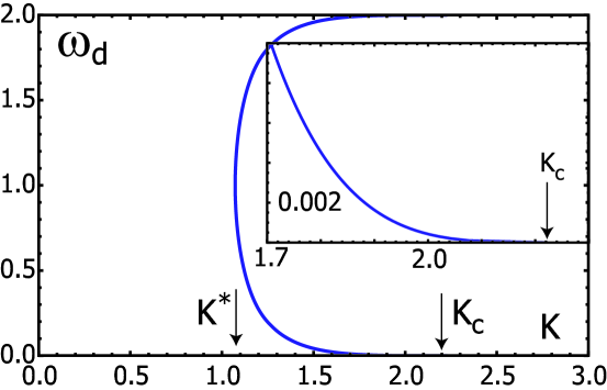
The study of the spontaneous emergence of a finite width can be done using the same directed polymer technique that we used in the previous section. Before we get into the details of this derivation it is useful to summarize the results that we shall obtain. When the levels have zero width, they are discrete. The curve defines the spontaneous appearance of a finite width. is equal to the (zero-temperature) critical coupling where the system becomes superconductor: . For finite , ; the minimal value of as function of occurs in the middle of the band, at . At the relaxation rate is zero for all states. This regime corresponds to the superinsulator introduced in Basko2006 . For a given intermediate value of the coupling , the states in the middle of the band have a finite width. They are separated from the states of zero width by a critical energy (obtained by inverting the function ) similar to the mobility edge of the non-interacting problem.
We now derive these results using the mapping to directed-polymers. The partition function of the directed polymer on the tree is now:
| (61) |
The computation of is deduced from the evaluation of the function
| (62) |
In the directed polymer terminology this problem turns out to be always in the low temperature phase corresponding to replica symmetry breaking, where the main contribution comes from a very small number of paths. This is due to the fact that always has a minimum at . As a consequence, one finds, using the same approach as in Sect.III.3: .
When one has , where is given in (10). Therefore, in the whole insulating regime one gets . Thus, the relaxation rate at very low frequencies decreases away from the boundary, in the bulk of the sample the width of levels is zero.
Let us now study the case of non-zero frequencies. The critical line at which a finite level width appears in the bulk of the sample is given by the two equations and which read:
| (63) | |||||
| (64) |
These equations can be written explicitly:
| (65) | |||||
| (66) |
where we have introduced the notation .
We begin by finding the region of the parameters in which the system of equations (63,64) has a solution. Clearly, the solution of these equations expressed as a function of is symmetric under at fixed . The energy corresponds to the minimal value of . For the equations (63,64) have no solution, so at these values of the cavity degree all energy levels have zero width in the bulk of the sample. At the system of equations (65,66) can be solved explicitly:
| (67) | |||||
| (68) |
Notice that for small the value is exponentially smaller than the value , given by (18), at which superconductivity appears.
Next, we consider the region of small . To solve the system (65,66) in this limit, we first notice that at the solution of the equations gives the critical point discussed in Sect.III.4: and . At small and the exponent should remain small: which allows us to neglect terms linear in in (65,66):
| (69) | |||||
| (70) |
The second equation (70) shows that scales as so deviations of from its critical value can be neglected in the first equation where terms linear in cancel. This gives
| (71) |
This reduces to a power law behavior of when is close to and :
| (72) |
These results are illustrated by Fig. 8 which shows as function of .
Note that the previous analysis shows that the region of small gives a negligible contribution to . This gives an a posteriori justification to the fact that we have neglected the non-perturbative modifications of the equation (60) in our study of the insulating phase.
IV.2 Scaling of the level width close to the transition.
The level widths strongly depend on the frequency for . The form of this dependence is important for the study of low temperature properties discussed below. To find we need to rederive the equation (60) for the case of non-negligible . The computation using the Keldysh formalism, which we shall explain in Section IV.3 below, gives at zero temperature:
| (73) |
As one expects, the decay rate of the state provides the cutoff of the divergence at This equation is similar to the equation (7) for the fields appearing in the superconducting phase. We are interested in the scaling of the typical level width for but close to the transition.
We will analyze this scaling with the same method as in Sect. III.6, in the RSB region. The crucial ingredient is the distribution of widths . We shall assume that it has a power law form with an upper cutoff :
The non-linear mapping (73) gives a self-consistent equation for this distribution. Performing the same steps as those used in the derivation of Eq.(44), we get:
| (74) |
where the function , defined by:
| (75) |
reduces to when . The mapping (73) implies that values much larger than are very rare. Indeed, such a value of at one step induces a much smaller value at the next step. We thus assume . Evaluating both sides of Eq. (74) we find
| (76) |
Close to the critical point , the exponent . Expanding at small we find using the Eq.(72) that
| (77) |
Finally, we obtain for the typical level width:
| (78) | |||||
| (79) |
As we shall discuss below, this fast energy dependence of the level width has important consequences for the low-temperature transport properties. As before, the numerical coefficient cannot be determined analytically because we do not know the precise value of . We emphasize that, according to Eq.(79), the energy scale in the exponent is much larger than the threshold energy . This inequality is valid in the whole range of validity of Eq. (79), as long as . Qualitatively, it leads to a very sharp growth of the typical level width right above the threshold.
The estimate of the level width close to the quantum critical point, , requires a special treatment because the expansion (77) and the final result (78) are valid only for frequencies close to the threshold so that . Thus, they are not applicable at the critical point where both and vanish. An approximate expression for in this regime should be found differently. First, using the function given by Eq. (72), we determine the inverse function for low :
Next, we substitute this expression into Eq. (76) and find
| (80) |
where is some function of only. At we find .
IV.3 The effect of a non-zero temperature on the level width.
In this section we derive the cavity equations for the level width within the Keldysh formalism. This allows to study the effect of a non-zero but low temperature. A low temperature affects the relaxation rate in several ways. First of all, it changes the occupation numbers of the excited states and the ground states; this affects the perturbative equation (60) and thus shifts the position of the line. This effect is however small at A more important effect is that, in the intermediate phase , a non-zero temperature induces a small number of mobile excitations with frequencies above . These excitations provide a mechanism for a small but non-zero level broadening for the levels even at very low frequencies, .
The effect of a small number of mobile excitations can be estimated qualitatively by the following arguments. The excitation with energy moves with a typical rate from site to site. Thus, with exponential accuracy a typical site sees a mobile excitation with energy passing by with rate The dominant contribution to the relaxation of this site comes from the energies . It results in the temperature dependence that shows a crossover between a behavior and an Arrhenius behavior as one goes away from the critical point.
We shall now use the Keldysh formalism to support these qualitative reasoning.
IV.3.1 Cavity equations for the relaxation rate: derivation with the Keldysh formalism.
As a first step, to be used later in the cavity approach, we begin with a study of a reduced two-spin system where a fluctuating field is coupled to spin . The Hamiltonian describing this system is
| (81) |
We need to find the effective relaxation rate of spin . For this we employ the Jordan-Wigner transformation, using Fermion creation operators and :
| (82) | |||||
| (83) |
The Keldysh action obtained after averaging over the environment variables is:
| (84) | |||||
| (85) |
Here subscripts are Keldysh indices corresponding to fermions moving forth or back in time. It is convenient to rotate all fermion vectors in the Keldysh space according to the Larkin-Ovchinnikov prescription (for details of Keldysh formalism see the recent detailed review KamenevReview ). For each we define
| (86) | |||||
| (87) |
After this rotation, the action acquires the form
| (88) |
where . The Fourier-transform of the matrix is a standard triangular matrix in Keldysh space:
| (89) |
The functions , and are respectively the retarded, advanced and Keldysh component of the matrix . If we denote by the spectral density of the external noise acting on spin , they are given by
| (90) |
Our goal is to determine the spectral density of noise acting on spin . The bare retarded fermionic Green function at site (in the absence of the coupling to site ) is
| (91) |
The action (88) is quadratic; diagonalizing it we get the imaginary part of the retarded fermionic Green function at site :
| (92) |
Here are the eigenvalues of the two-spin Hamiltonian (81) in absence of the fluctuating field. In the following we shall neglect the effects of level repulsion which translates into the difference between actual energies and their unperturbed values . This is the same approximation that we employed in Sect. III to obtain analytical results. As we have shown above, this approximation remains accurate even for very modest values of . Using this approximation we can rewrite (92) as
which implies that the imaginary part of the self-energy is
| (93) |
as one expects from perturbation theory arguments.
At zero temperature these results for the fermion Green function are translated directly into spin correlators. At non-zero temperature this conversion is less trivial because the spin correlators acquire an additional decay compared to fermions. Physically, this is due to the fact that the spin Hamiltonian is non-linear, so the thermal excitation of one spin might lead to the relaxation of another spin. For this process to happen the thermal excitation should be mobile, meaning that it should have an energy larger than This makes such processes rare at low temperatures. Formally, the retarded transverse spin Green function at site , denoted as , differs from the retarded fermion Green function, , because the former contains an additional factor due the non-linearity of the Jordan-Wigner transformation. More precisely, in Keldysh technique these two Green functions are related by
| (94) |
The dynamics of the -spin components is purely dissipative in the leading order in which we consider here. In this approximation the retarded Green function of the -spin components is zero; this allow us to neglect the second term in the general expression (94) for . The first term has two parts: where and is the irreducible part of the symmetrized spin-spin correlator at site :
| (95) |
In the following we shall be mostly interested in the relaxation at low energies . Combining Eqs.(94,95) and (91), we get the equation for the imaginary part of the retarded transverse spin-spin correlator at site at non-zero temperature:
| (96) |
Here is the relaxation rate at ; it coincides with given by Eq.(93). Below we neglect the level widths compared to level energies, which allows to find the imaginary part of the inverse transverse spin correlation function at site , i.e. the relaxation rate of the spin at site :
| (97) |
The second term in this equation is due to the non-linearity discussed above; in this term we have neglected the contribution of compared to . The reason for this is that this term is exponentially small at low due to the factor Thus, this term makes a significant contribution only if the energy of spin is large: , so that is much larger than .
The result (97) describes the relaxation in the system of two spins. We now consider a full cavity problem in which spin has neighbors, labeled , and each of these neighbors feels a fluctuating external field with spectral density . We compute the relaxation rate of the spin at site . Adding the contributions from all neighbors we get
| (98) |
In the zero temperature limit the second term in (98) vanishes and this formula reduces to (73).
At non-zero temperatures, one needs to take into account the second term in (98), which becomes important for low frequencies for which would be zero at . In this regime the second term works as a source term to the recursion that would otherwise give zero.
IV.3.2 Solution of the recursive equations with a source term and consequences for low temperature properties.
At non-zero temperature the low energy modes which are discrete at acquire a finite lifetime. We shall estimate their broadening at very low temperature when the effect of non-zero on modes with can be neglected. Our starting point is equation (98) which contains two terms of very different physical meaning. The first term describes the decay due to the indirect coupling to the external fields far away, it is the only term present at . The second term describes the relaxation caused by mobile thermal excitations of a neighboring spin with energy above the threshold . At low temperatures such excitations occur exponentially rarely and thus are essentially limited to a narrow range of energies slightly above . Because the density of these excitations is very low, we can ignore the situations in which a given site feels more than one thermal excitation nearby. It implies that the relaxation rate induced by these excitations for low-energy modes is much smaller than the rate of the mobile excitations. This allows us to replace the effect of the mobile excitations on low energy modes by an effective fluctuating field. As we shall see below the spectrum of this field is featureless, so in all respects the mobile excitations are similar to the external field.
The approximation discussed above allows us to replace the relaxation rate in the second term in (98) by its typical value and to ignore the effect of a non-zero temperature on this term. Eq. (98) becomes very similar to Eq.(48) for the susceptibility:
| (99) | |||||
where is given by the zero-temperature result, see Eq.(78). The dominant contribution to the external dissipation in Eq.(99) is determined by the competition between and . Evaluating the integral over in the saddle point approximation (valid under the conditions and ) we find that is weakly -dependent and given by
| (100) |
The estimate (100) is valid with exponential accuracy provided that . The weakness of the frequency dependence in proves our statement above according to which the noise produced by the thermal excitations is featureless and exponentially small.
Using the formal analogy between Eq.(99) and the Eq. (49) for the susceptibility, we can now use the results obtained in Sec.III.8. The key conclusion of this section that we need here is that the typical value of the susceptibility does not contain any divergence at the transition point. This implies that the typical sub-threshold level width is . This confirms our conjecture above that the relaxation rate of the low energy modes is very low, which allowed us to replace the mobile excitations by an effective fluctuating field. To estimate the level width for the whole range of frequencies, we note that both and (see Eq.(78)) are exponentially fast functions, therefore
| (101) |
The estimates (78) and (100) are not valid right at the critical point , where and vanish and the level width is given by Eq.(80). Repeating the calculations similar to those used to derive Eq.(80) we find at , instead of (100):
| (102) |
The equations (100,102) give the typical relaxation rate of low energy modes. At the same time they give a typical noise level and thus a typical rate of transport processes in this model. For the superconductor-insulator transition the result (100) implies that, away from the critical point, the resistivity follows the Arrhenius law at very low temperatures and a law in the intermediate temperature regime. This behavior is exactly opposite to the one expected and observed in conventional Mott insulators where Arrhenius is followed by Mott behavior as temperature is decreased. Exactly at the critical point, the resistivity grows as a stretched exponential with for a physically relevant .
V The effect of frustration.
Disordered superconducting films close to the SI transition can be driven to insulators by the application of a magnetic field. The properties of these materials in presence of a magnetic field have been extensively studied experimentally and are rather unusual. So it is important to discuss the theoretical expectations. We will not undertake a full quantitative study here, but we will only study the leading effects of a magnetic field on the phase diagram of our model formulated on the Bethe lattice. In the framework of this model the effect of a magnetic field is described by the effective model where nearest-neighbor couplings defined in Eq.(1) acquire random phases: , with . The effects of these random phases on the two major lines of our phase diagram (see Figs. 2 and 8), the critical temperature line and the threshold energy line in the insulating phase , are crucially different. Whereas all the equations for level widths contain squares of absolute values of matrix elements only, and thus do not depend on , the equations for the order parameter are affected by the random phases.
Consider first the case of small phase fluctuations . In the limit of very large the simple mean-field approximation should be valid, and the transition temperature is determined by the equation for the first moment of the distribution. Random phases enter this equation via a straightforward modification of the coupling strength, , which leads to the suppression of :
| (103) |
Because is small, the suppression of the transition temperature (and therefore the decrease of the typical order parameter in the ordered phase) can be rather strong even at .
The case of strong frustration is more complicated. Here we consider the limit of very large fields that generate completely random phases with uniform distribution over . Instead of Eq.(7) we get
| (104) |
and we look for a solution for the distribution function which depends only on the absolute value .
In order to determine we use the linearized version of (104) which can be rewritten in terms of the Fourier transformed distribution . We shall assume that this Fourier transform depends only on the absolute value : . It then satisfies:
| (105) |
Note that these equations are formally identical to those obtained in the case without magnetic field in (29). However, the analytic properties expected in the present case are different: the random phases induce a symmetric distribution, instead of the distribution supported on positive ’s when there is no magnetic field. We will look for a power-law solution of Eq. (105) at small in the form .
Because the average order parameter is zero in the limit of large magnetic fields, the simple mean-field solution is obtained by assuming that is determined by its second moment and correspondingly . The self-consistent equation (105) then gives . This is the equivalent of (4) in the zero magnetic field case.
The equation for the Laplace transform (105) is formally identical to the one obtained in zero field (29), so the value of the exponent that determines the behavior of the Fourier transform at small is determined by the same equations (23,24) derived in Sect. III.4. The important difference between the cases of zero and large magnetic field is due to the fact that in the latter case the simple mean field solution corresponds to . As a result, in contrast to zero field case, the simple mean field solution is not valid even in the limit. In other terms, RSB always occurs for the fully-random problem defined by Eq. (104).
We begin by solving these equations in the large limit, where the exponent approaches , with as long as . Assuming that , we can extend the integrals over in Eqs.(23,24) up to . We estimate the resulting integrals:
and obtain
| (106) | |||||
| (107) |
Similarly to the zero magnetic field case, in the RSB phase the naive mean field prediction is exponentially larger than the correct result (107) for small .
We now prove that for any the transition occurs in a RSB phase. To find the temperature, corresponding to replica symmetry breaking we consider the Eq. (24) and assume that , using a procedure similar to the determination of the RSB point, Eq.(21), discussed in Sec.III.4 for the unfrustrated case. However, in contrast to the zero-field case, the corresponding temperature , is always above the simple mean field value at . Thus, it is necessary to solve both equations (23,24) together to determine the value of the exponent and transition temperature.
The applicability of the solution (106,107) is limited to the regime of very large , when is so small that the corrections of order due to the finite upper limit in the integral are negligible. When decreases these corrections become significant and the exponent starts to decrease; it eventually approaches unity at the value determined in Eq.(21). At the same time, deviates from the simple law (106) and attains at its maximum value, equal to the mean-field transition temperature of the unfrustrated model. At still smaller , the solution for is identical to the one discussed in Sec.III.4 for the unfrustrated model. This behavior is summarized in Fig.9.
Although the transition line stays the same (in the RSB phase) for the unfrustrated model and for the strongly frustrated one, the amplitudes of the order parameter in the ordered phase differ considerably. This is illustrated by the numerical solution of the random-phase mapping equations (104) shown in Figs. 10 and 11 for zero temperature and near to the quantum critical point .
The results shown in Fig. 11 are very much like those seen in Fig. 3 for the unfrustrated model, but the typical amplitude is suppressed by a factor in the frustrated case at the same value.
To summarize this section, we have demonstrated that frustration suppresses strongly the transition temperature when one is in the replica symmetric phase at sufficiently large but it has no effect on in the RSB phase near the quantum phase transition. This can be interpreted as a consequence of the quasi-one-dimensional nature of Bethe-lattice clusters which contribute to the formation of the coherent state in the RSB phase. While is unchanged in the RSB region, the amplitude of the order parameter (at ) is strongly suppressed due to frustration, as demonstrated in Fig. 11. More work is needed to decide if these results, obtained on the Bethe-lattice problem, can be applied to the finite-dimensional problem where closed loops are present (see discussion in section VI.3). We expect, however, that the results will remain qualitatively similar due to the dominance of a small number of paths that makes the presence of small loops largely irrelevant.
VI Consequences for experiments.
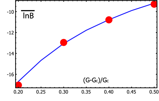
VI.1 Distribution of coherence-peak heights in STM and Andreev point contact tunneling experiments.
One of the main results of this work is anomalous broadening of the distribution of the local values of the order parameters in the vicinity of the SI transition. This conclusion can be tested by STM measurements.
The same STM experiments can also confirm that the transition happens due to Cooper pair localization and not by unbinding of Cooper pairs. In a usual setup of these experiments one measures the current-voltage characteristic of a highly resistive tunneling contact between the material and a needle of the STM machine. The measured differential conductance, , is proportional to the single-electron density of states, , at energy . Thus, these measurement directly probe the superconducting gap. The experiments performed on superconductor-insulator transition in TiN Sacepe2007 ; Sacepe2009 and InO Sacepe2007 ; Sacepe2010 demonstrate that in these materials the superconductor-insulator transition happens without pair destruction (the single-electron gap remains large). The theoretical justification of this was given in the workFeigelman2010 and is summarized above in section II.1. Thus, one expects that this transition is driven by the competition between disorder and Cooper-pair tunneling and is described by the models studied in this paper. As we discussed in section II.1 the present paper ignores subtle effects of the correlations between matrix elements, in this approximation the disorder changes only the number of neighbors, . In order to compare with experimental data we need to choose the interaction constant so that to reproduce the correct value of away from the transition in these materials. This gives the interaction used in many numerical plots in the previous sections.
In superconductors the density of states above the gap displays the coherence peak which is due to the superconducting order parameter. The height’s statistics of these peaks can be used to measure the variations of the local order parameter appearing in the vicinity of the superconductor-insulator transition. In particular, the broadening of the distribution translates into the broad distribution of peak heights. This theoretical prediction was indeed confirmed in very recent experiments Sacepe2010 where superconducting samples with different values of were studied and compared. The data shows that while the superconducting gap remains largely intact in lower samples and experience modest fluctuations from point to point, the distribution of peak heights changes dramatically as the insulator is approached. This observation is in full agreement with the theory developed in this work, and confirms our expectation that the solution of the model on Bethe lattice provides a good approximation for the properties of realistic physical systems.
Another possible set of data is given by Andreev point-contact tunneling measurements. Similar to conventional tunneling, these experiments give current-voltage characteristics of the point contact. However, in contrast to conventional contacts, the contacts used in these experiments are characterized by a small resistance, . This allows a coherent tunneling of the Cooper pair between the normal needle and a superconducting material.
In a conventional BCS superconductor the differential conductivity observed in Andreev point-contact experiments shows a suppression below the single-particle gap and a peak at the gap edge, similar to the conventional tunneling. The reason for this is that in conventional superconductors the gap, , for collective pair excitations (pseudospins) is exactly twice as large as the gap for single particle excitations: . Tunneling of Cooper pair brings energy , so the gap edge observed in differential conductivity for the single particle tunneling coincide with the one observed in Cooper pair tunneling.
In contrast to conventional superconductors, strongly disordered superconductors in the vicinity of the SI transition are expected to show much smaller gap for collective pair excitations, , than the one characterizing single-particle tunneling, . In this case, the observed differential conductivity below single-particle gap is due to the coherent Cooper pair tunneling which might occur at potential differences . In the lowest non-zero order in tunneling one gets that at such bias the differential conductivity is proportional to the local susceptibility, , of the equivalent spin model evaluated at the position of the needle, . This expectation is correct provided that the collective modes contributing to the local susceptibility are delocalized at this frequency. The tunneling into localized modes cannot lead to experimentally observable conductivity. Because the energy separating the localized and delocalized modes is the same at different positions in the sample, we expect that the observed differential conductivity is characterized by a spatially uniform threshold or a peak. This expectation is in agreement with the preliminary results Dubouchet2011 .
VI.2 Low-temperature resistivity in the insulating state
Because STM measurements require that the resistance of the tunneling contact is much larger than the resistance of the sample, they become difficult, if not impossible, in the insulating phase. So, in this state one should compare the theoretical predictions with the transport data which are always more difficult to interpret. The most striking feature of the resistivity on the insulating side of the transition in InO and TiN is the activated behavior of the resistance , with an activation energy that decreases in the vicinity of the transition. SacepeShahar2009 ; Sacepe2008 This decrease of the activation energy, , is in contrast with a large and non-critical single particle gap observed in STM Sacepe2007 ; Sacepe2009 ; Sacepe2010 on the superconducting side of the transition. It indicates that the transport in this regime is due to incoherent Cooper pair hopping. More direct evidence of the pair transport is provided by the data on magnetoresistance oscillations in perforated films which displays periodic oscillations with “superconducting” flux period in the insulating state.Valles2009
As we have shown in Section IV.1, the low lying excitations of the spin model have zero width. This translates into the localization of all excitations with energies . The transport is made possible by modes with energies which become thermally excited at non-zero temperatures. Thus, we expect that the resistivity in this state has an approximately activated temperature dependence at lowest temperatures with an activation energy which decreases when one approaches the transition. The subdominant term in the resistance is proportional to which might become important at intermediate temperatures because . This result is in agreement with the data. It should be contrasted with the naive expectation according to which the transport of Cooper pairs could be characterized by Mott (or Efros-Shklovskii) behavior, giving a behavior ( in analogy with single electron transport in conventional insulators. In these insulators the activation behavior is realized at intermediate temperature range and Mott behavior at lowest temperatures.
The sharp boundary, , separating the localized and delocalized modes could be more directly probed by microwave experiments. We expect that close to this boundary the lifetime of the excitations becomes very long. Thus, even a weak microwave radiation could excite a large number of these excitations. This would dramatically increase the conductivity of the sample without affecting significantly its temperature. Furthermore, applying the microwave power in pulses with varying time intervals between the pulses, one could obtain information on the lifetime of these excitations near the many-body mobility edge.
VI.3 The effect of frustration induced by a magnetic field or by unconventional order parameter symmetry.
As discussed in Section V, the highly inhomogeneous spatial structure appearing in the vicinity of the SI transition strongly suppresses the effects of frustration and thus of a magnetic field. In the approximation used in this work the magnetic field has no effect on the transition temperature in this phase. The account of higher order effects in would lead to a small suppression of the critical temperature in this regime. This conclusion is in qualitative agreement with the data: it has been found (see e.g. Sacepe2007 ; Sacepe2008 ; Sacepe2009 ; Sacepe2010 and references therein) that the properties of the materials depend very sensitively on the disorder level in the vicinity of the SI transition in contrast to their smooth dependence on a magnetic field. In spite of its weak effect on the transition temperature, we have observed that the magnetic field should affect strongly the order parameter. This prediction can be tested by STM and Andreev point-contact measurements which provide direct information on the local superconducting order parameter and its distribution.
The very weak effect of a magnetic field on the transition temperature implies that superconductivity might survive in strongly disordered superconductors with unconventional pairing symmetries such as d-wave symmetry, provided that the Cooper pairs in these superconductors are formed on very short scales which are weakly affected by disorder. This might be the case in high superconductors in the pseudogapped regime in which there are reasons to expectGeshkenbein1997 ; Galitski2009 that electrons are paired in the corners of the Brillouin zone. In this case the Cooper pairs have very small size and are not affected by disorder. The global superconductivity is due to the coupling between these localized Cooper pairs. These couplings have random signs due to the d-wave symmetry of the order parameter which makes this situation similar to the strongly disordered superconductor in a magnetic field. As discussed above the randomness of the couplings has weak effect on the transition temperature. This might explain the apparent similarity between underdoped high superconductors and strongly disordered InO and TiN films, noted by many researchers previously, see for example Steiner2005a ; Steiner2005b
VI.4 Change of level statistics: suggestion for numerical work.
The many-body mobility edge line found in Section IV.1 divides the parameter space of the Hamiltonian into regions with qualitatively different spectral statistics. At the spectrum is point-like and the many-body wavefunctions are localized, thus we expect the level statistics to be Poissonian in this region. On the other hand, above the mobility edge, at , a nonzero line width is generated, indicating the extended nature of wavefunctions. In this regime we expect a Wigner-Dyson level statistics, with level repulsion. This change of level statistics can be studied numerically via exact diagonalization of the Hamiltonian (1).
A similar study was implemented recently in the workHuse2007 for a one-dimensional model of interacting fermions. This paper has found a qualitative evolution between Poissonian and Wigner-Dyson statistics, but large finite-size effects make any quantitative conclusions difficult in the absence of an appropriate analytic theory. We expect that the Hamiltonian (1) with moderate branching number could be useful for such study, because our theoretical predictions for the position of the mobility edge can be used for comparison with the numerical data.
As a next step, it would be important to extend such a numerical study to the same type of quantum spin models on a usual real-space lattice. The comparison of the results for spectral statistics obtained on conventional Euclidean lattices and on the Bethe lattice could be very useful to check the applicability of the approach developed in this paper to physical systems.
VII Conclusions
In conclusion, we have outlined a solution of the strongly disordered spin model on the Bethe lattice that can be mapped onto the disorder-driven superconductor-insulator transition or onto the disordered ferromagnets. We found a series of two zero temperature transitions between an ordered state, a state with a slow relaxation and a state with no relaxation. Our solution also shows that the low temperature phase in this model is always very strongly non-uniform with both the order parameter formation and the spin relaxation controlled by rare paths that contain a very small fraction of spins. When applied to the superconductor-insulator transition our results imply the existence of both weak and strong insulators. In the former the relaxation rate varies faster, as , in an intermediate temperature range, but it crosses over to Arrhenius at very low temperatures. Exactly at the quantum critical point we expect a relaxation rate that varies as with a non-universal that depends on the interaction constant. For physically relevant values of the interaction constant we expect .
In the strong insulator the relaxation is completely suppressed. Of course, the physical effects neglected in our model (like electron-phonon coupling) would lead to some slow relaxation even in the latter phase.
The predictions of our theory can be tested by conventional STM experiments and Andreev point-contact tunneling experiments on superconducting films of InO and TiN as discussed in detail in Section VI.
In the strongly insulating phase the local quantum levels remain discrete, this implies that such systems would remain coherent for a very long time (limited by the interaction with phonons and other environment neglected in our model). When applied to disordered magnets this result implies that a stronger disorder might make the spin system less noisy and more coherent. This might be important for the efforts to suppress the flux noise in superconducting circuits where it is believedFaoro2008 ; Koch2007 to be due to the disordered spins at the surface of the superconductors.
Our theory is directly applicable to the models on Bethe lattices which do not have small loops. Qualitatively it looks very likely that the dominance of a small number of paths, which is a central result of this work, implies that small loops are irrelevant and therefore the Bethe-lattice approximation should be very good. This conjecture might be checked numerically (see Section VI.4).
We now briefly discuss possible extensions of the present theory and list few open problems:
-
•
Extension of the developed technique to the spin lattices in Euclidean space. It is believed that the exponential behavior of physical properties in the localization problem on a Bethe lattice disappears in any finite dimensionMirlin1994 . However, the arguments of Mirlin1994 are not directly applicable to the non-linear problem of phase transition that we consider here in which the phase-space dimension increases exponentially with the number of sites. Qualitatively it seems likely that the dominance of a small number of paths is an indication that the main results of the Bethe-lattice approximation will remain correct in finite dimensions.
-
•
The extension to finite-dimensional systems would be greatly simplified if one could find the appropriate order parameters for the phase transitions found on Bethe lattice. In particular, these order parameters should describe not only the appearance of the superconducting order but also its homogeneity and its time-reversal symmetry breaking which appears at the second transition.
-
•
Direct calculation of transport quantities such as thermal conductivity or electrical resistivity near the quantum transition studied in this work. The present paper computes the spin relaxation time which for the SI problem translates into the time required for the Cooper pair to move away from a given site. With exponential accuracy it should be the same as the resistivity or thermal conductivity in the system. In order to compute the properties with better accuracy one would need to develop the formalism to compute transport properties directly in this problem.
-
•
Direct computation of the dynamic spin susceptibility . The behavior of this quantity determines the pair conductivity measured in STM experiments and Andreev contact spectroscopy.
-
•
Finite temperature effects in the strong insulator. In the approximation used in this paper even a high temperature has no effect on the strong insulator. However, one might worry that our approximation might miss exponentially small effects such as rare regions characterized by larger density of states that would make this part of the system less insulating.
VIII Acknowledgments
We acknowledge useful discussions with G. Biroli, C. Chapelier, T. Dubouchet, V. Kravtsov, M. Mueller, F. Zamponi and B. Sacepe. This work was supported by Triangle de la physique 2007-36, ANR-06-BLAN-0218, ECS-0608842, ARO 56446-PH-QC, DARPA HR0011-09-1-0009 and by the program "Quantum physics of condensed matter" of the Russian Academy of Sciences, and RFBR grant 10-02-00554.
IX Appendix A: Quantum cavity method: Suzuki-Trotter formulation and further approximations
If one is interested only in the thermodynamic properties of the problem described by (1,2) on the Bethe lattice (a random graph of connectivity ), one can write Laumann an exact (at the replica symmetric level) cavity recursion in terms of Suzuki-Trotter paths. Unfortunately this exact recursion can be studied only numerically and is rather heavy to handle in the case of disordered systems. Our approach uses a simplified version which amounts to using a special measure on the Suzuki-Trotter paths. In this appendix we briefly summarize the exact cavity recursion and we make explicit the extra approximations of our method. Let us study for instance the transverse-field Ising Hamiltonian (2).
| (108) |
The partition function can be expressed with the Suzuki-Trotter representation. Using imaginary time steps, one introduces the time trajectory of each spin, , where . Then
| (109) |
where:
| (110) |
and
The exact RS method introduced in Laumann is the following: take a branch of the Bethe lattice rooted on spin , and define the probability distribution of the time-trajectory of this spin as . Let us define analogously, for each of the spins j which are the first neighbors of i on the rooted tree, their time trajectory as . Then one can write formally the mapping that generates, from the new . This mapping is then typically studied numerically by a population dynamics method where one represents each of the by a sample of spin trajectories. In paper Krzakala it is shown how to take the limit by using a continuous time formulation where one memorizes only the times at which the spin trajectories jump. The whole procedure can be seen as a two-step approach: transforming the problem to one of classical spin trajectories, and then using the classical cavity method MezardParisi2001 . In particular, the cavity mapping can be shown to derive from a variational principle based on a Bethe free energy.
The quantum cavity approach that we have introduced in Sect. III.2 can be understood as an approximate way to study the exact RS Suzuki-Trotter based cavity method. Basically, the hypothesis amounting to using a local Hamiltonian of spin in the form amounts, in the Suzuki-Trotter formalism, to using a local distribution which takes the special form
| (111) |
This form can be used with different methods. In a variational approach one injects this form into the Bethe free energy. This gives a free energy which depends on all the parameters , on which one should optimize. In practice this method is a bit heavy numerically because the computation of this Bethe free energy as function of the involves, for each spin , a trace over and all its neighbors , which is thus a sum over terms. In the approach that we have described in Sect. III.2 we use a slightly different method: we suppose that all the cavity neighbors of a given spin have distribution . From these distributions we compute and deduce from it the value which reproduces this average. This defines a mapping from to . This type of approach can be tested by comparing it to the full numerical sampling of Suzuki-Trotter trajectories in the case of a uniform transverse field where . This study, done in Zamponi , confirms that this approach is able to reproduce the phase diagram accurately (the variational approach is a bit more precise, but both approaches give the zero-temperature value of within a few per-cent).
Our approach uses one more step of approximation: instead of the quantum cavity mapping described above, we have mostly used the explicit mapping (7) which has the advantage that one does not need to compute in order to find the value of . The validity of this further step of approximation has been studied in Sect.III.7.
References
- (1) S. Sachdev, Quantum Phase Transitions, Cambridge University Press (2000).
- (2) D. M. Basko, I. L. Aleiner, and B. L. Altshuler, Ann. Phys. 321, 1126 (2006).
- (3) M. Ma and P. A. Lee, Phys. Rev. B 32, 5658 (1985).
- (4) M. Ma, B. Halperin and P. Lee, Phys. Rev. B 34, 3136 (1986).
- (5) S. Ma, C. Dasgupta and C. Hu, Phys. Rev. Lett. 43, 1434 (1979); C. Dasgupta and S. Ma, Phys. Rev. B 22, 1305 (1980)
- (6) D.S. Fisher, Phys. Rev. Lett. 69, 534 (1992); Phys. Rev. B 50, 3799 (1994).
- (7) L.B. Ioffe and M. Mézard, arXiv:0909.2263, to appear in Phys. Rev. Lett.
- (8) M. Mueller, Ann. Phys. (Berlin) 18, 849 (2009); arXiv:0909.2260
- (9) A. Goldman and N. Markovic, Phys. Today 51, 39 (1998)
- (10) V. F. Gantmakher and V. T. Dolgopolov, Phys. Usp. 53, 1 (2010)
- (11) A. F. Hebard and M. Paalanen, Phys. Rev. Lett. 65, 927 (1990).
- (12) G. Sambandamurthy, L. W. Engel, A. Johansson, and D. Shahar, Phys. Rev. Lett. 92, 107005 (2004).
- (13) M. A. Steiner, N. P. Breznay and A. Kapitulnik Phys. Rev. B 77, 212501 (2008).
- (14) B. Sacepe Ph. D. Thesis, CEA-Grenoble (2007).
- (15) B. Sacepe, C. Chapelier, T.I. Baturina, V.M. Vinokur, M.R. Baklanov, M. Sanquer, Phys. Rev. Lett. 101, 157006 (2008).
- (16) B. Sacepe, C. Chapelier, T. I. Baturina, V. M. Vinokur, M. R. Baklanov, M. Sanquer, arxiv:0906.1193
- (17) B. Sacepe, T . Dubouchet, C. Chapelier, M. Sanquer, M. Ovadia, D. Shahar, M. Feigel’man and L. Ioffe, to be published.
- (18) C. Howald, P. Fournier, and A. Kapitulnik, Phys. Rev. B 64, 100504 (2001).
- (19) S.H. Pan, J.P. O’Neall, R.L. Badzey, et al., Nature 413, 282 (2001).
- (20) K.M. Lang, V. Madhavan, J.E. Hoffman, E.W. Hudson, H. Eisaki, S. Uchida, J.C. Davis, Nature 415, 412 (2002).
- (21) K.K. Gomes, A.N. Pasupathy, A. Pushp, S. Ono, Y. Ando, A. Yazdani, Nature 447, 569 (2007).
- (22) M. V. Feigel’man, L. B. Ioffe, V. E. Kravtsov and E. Cuevas, Annals of Physics 325, 1368 (2010); arXiv:1002.0859
- (23) H. van Der Zant, W. J. Elion, L. J. Geerling and J. E. Mooji, Phys. Rev. B 54, 10081 (1996) .
- (24) R. Fazio, H. van der Zant, Phys. Rep. 355, 235 (2001).
- (25) E. Serret, Ph.D. Thesis, CNRS-Grenoble (2002).
- (26) P. W. Anderson, J. Phys. Chem. Solids 11, 26 (1959).
- (27) L. N. Bulaevskii and M. V. Sadovskii, Pisma ZhETF 39, 524 (1984); L. N. Bulaevskii and M. V. Sadovskii, J.Low Temp.Phys. 59, 89 (1985); M. V. Sadovskii, Phys. Rep, 282, 225 (1997).
- (28) A. Kapitulnik and G. Kotliar, Phys. Rev. Lett. 54, 473 (1985); G. Kotliar and A. Kapitulnik, Phys. Rev. B 33, 3146 (1986).
- (29) A. Ghosal, M. Randeria, and N. Trivedi Phys. Rev. B 65, 014501 (2001).
- (30) Z. Ovadyahu, private communication.
- (31) V. Anisimov, private communication.
- (32) M. Mézard and G. Parisi, Eur. Phys. J. B 20, 217 (2001).
- (33) C. Laumann, A. Scardicchio and S. L. Sondhi Phys. Rev. B 78, 134424 (2008).
- (34) F. Krzakala, A. Rosso, G. Semerjian and F. Zamponi, Phys. Rev. B 78, 134428 (2008).
- (35) B. Derrida and H. Spohn J. Stat. Phys. 51, 817 (1988)
- (36) J. Cook and B. Derrida J. Phys. A 23, 1523 (1990).
- (37) M. Mézard, G. Parisi and M. Virasoro “Spin Glass Theory and Beyond”, World Scientific, Singapore (1987).
- (38) B. Derrida, Phys. Rev. B 24, 2613 (1981)
- (39) D. J. Gross and M. Mézard, Nucl. Phys. B 240, 431 (1984)
- (40) T. Dubouchet, B. Sacepe, C. Chapelier, M. Sanquer, M. Ovadia and D. Shahar, to be published.
- (41) M. Ovadia, B. Sacepe, D. Shahar, Phys. Rev. Lett. 102, 176802 (2009).
- (42) H. Q. Nguyen, S. M. Hollen, M. D. Stewart, Jr., J. Shainline, Aijun Yin, J. M. Xu, and J. M. Valles, Jr. , Phys. Rev. Lett. 103, 157001 (2009).
- (43) M.A. Steiner, A. Kapitulnik, Physica C 422, 16 (2005).
- (44) M.A. Steiner, G. Bobinger, A. Kapitulnik, Phys. Rev. Lett. 94, 107008 (2005).
- (45) V.B. Geshkenbein, L.B. Ioffe, A.I. Larkin, Phys. Rev. B 55, 3173 (1997).
- (46) V. Galitski, S. Sachdev, Phys. Rev. Lett. 79, 134512 (2009) .
- (47) V. Oganesyan and D. A. Huse, Phys. Rev. B 75, 155111 (2007)
- (48) A. Kamenev and A. Levchenko, Adv. Phys., 58, 197 (2009).
- (49) A. Mirlin and Ya. Feodorov, J. de Physique 4, 655 (1994).
- (50) L. Faoro and L.B. Ioffe, Phys. Rev. Lett. 100, 227005 (2008).
- (51) R. H. Koch, D. P. DiVincenzo and J. Clarke, Phys. Rev. Lett. 98, 267003 (2007).
- (52) F. Zamponi, private communication.