Many-Body Theory of Synchronization by Long-Range Interactions

Abstract

Synchronization of coupled oscillators on a $d$-dimensional lattice with the power-law coupling $G(r)=g_{0}/r^{\alpha}$ and randomly distributed intrinsic frequency is analyzed. A systematic perturbation theory is developed to calculate the order parameter profile and correlation functions in powers of $\epsilon=\alpha/d-1$. For $\alpha\leq d$, the system exhibits a sharp synchronization transition as described by the conventional mean-field theory. For $\alpha>d$, the transition is smeared by the quenched disorder, and the macroscopic order parameter $\overline{\psi}$ decays slowly with $g_{0}$ as $|\overline{\psi}|\propto g_{0}^{2}$.

Introduction.

Collective oscillations of active interacting elements are observed in a variety of physical, chemical, and biological systems far from equilibrium. Numerous studies have been devoted to the mutual entrainment of oscillators that have different intrinsic frequencies Kuramoto ; Strogatz00 ; Acebron . A class of models with global (or mean-field) coupling have enjoyed deep theoretical understanding Kuramoto75 ; Crawford99 . The phase of the oscillators become coherent as the coupling strength $g_{0}$ exceeds a threshold, which is the onset of synchronization. Extensive research has been focused on the transition behavior Kuramoto75 ; Crawford99 ; Daido94 ; Crawford95 ; Hong07 . The amplitude of the macroscopic order parameter scales as $|\overline{\psi}|\propto(g_{0}-g_{c})^{\beta}$, with $\beta=1/2$ for the original mean-field model by Kuramoto Kuramoto75 , while $\beta=1$ for some other types of coupling Crawford99 ; Daido94 ; Crawford95 .

Compared to the case of global coupling, behaviors of locally Sakaguchi87 ; StrogatzMirollo88 and non-locally Kuramoto95 ; Strogatz04 coupled oscillators are still widely open questions. In particular, knowledge about synchronization caused by long-range interactions is quite limited Rogers ; Marodi ; Zaslavsky , although they are ubiquitous in Nature in the form of, e.g., gravitational, electromagnetic, elastic, and hydrodynamic forces. Early numerical works for the power-law coupling $\propto 1/r^{\alpha}$ in $d$-dimensional array of oscillators show that global synchronization is possible for $\alpha\leq 2$ ($d=1$) Rogers , while system-size effect is significant for $\alpha\leq d$ ($d=1,2$) Marodi .

Recently, we proposed a simple model of microfluidic carpets hsync-paper1 ; hsync-paper2 , which is a two-dimensional array of rotors with a hydrodynamic coupling $\propto 1/r^{3}$. The model exhibits an unconventionally smooth transition to the synchronized state hsync-paper2 . The macroscopic order parameter decays gradually as the randomness is increased, in contrast to the sharp transition for global coupling.

Motivated by the numerical results, this Letter theoretically addresses synchronization of oscillators with a general class of long-range coupling. We will develop a systematic perturbation expansion around the mean field, taking the moments $\sigma_{n}$ of the interaction $G({\bf r})$ as the small parameters (which is analogous in spirit to the cluster expansion in the classical gas theory). For the power-law coupling $G({\bf r})=g_{0}/r^{\alpha}$, it is equivalent to a series expansion in $\epsilon=\alpha/d-1$. We will solve for the order parameter profile and correlation functions up to $O(\epsilon^{2})$. The main finding of this paper will be that the macroscopic order parameter for $\alpha>d$ behaves as $|\overline{\psi}|\propto g_{0}^{2}$ for $g_{0}\to 0$, which means that synchronization persists for arbitrary weak coupling. We interpret it as the result of quenched spatial heterogeneity. In contrast, for $\alpha\leq d$, the heterogeneity is averaged out and the transition is exactly described by the mean-field theory.

Model.

In our model, oscillators indexed by $i=1,2,\ldots,N$ are arrayed on a $d$-dimensional regular lattice with the unit grid size. The phase $\phi_{i}$ of the $i$-th oscillator located at ${\bf r}_{i}$ obeys the dynamic equation,

$$\frac{d\phi_{i}}{dt} = \omega_{i}-\sum_{j\neq i}G({\bf r}_{i}-{\bf r}_{j})\sin\left(\phi_{i}-\phi_{j}\right),\qquad$$ (1)

where $\omega_{i}$ is the intrinsic frequency that has the Gaussian distribution with the standard deviation $\omega_{0}$,

$$P(\omega_{i})=\frac{1}{\sqrt{2\pi}\omega_{0}}\exp\left(-\frac{\omega_{i}^{2}}{2\omega_{0}^{2}}\right).$$

We require the coupling function $G({\bf r})$ to be positive, slowly decreasing function of $|{\bf r}|$, so that its moments

$$\sigma_{n}=\sum_{j\neq i}G({\bf r}_{i}-{\bf r}_{j})^{n}$$

rapidly decays with $n$. To be specific, let us consider the power-law coupling $G({\bf r})=g_{0}/r^{\alpha}$ with the constants $g_{0}>0$ and $\alpha\geq 0$. We normalize the coupling by rescaling time so that $\sigma_{1}=1$ without losing generality. For the global coupling ($\alpha=0$), we have $G(r)=g_{0}=1/N$, and the moments $\sigma_{n}=1/N^{n-1}$ for $n\geq 2$ vanish as $N\to\infty$. In more general, for $\alpha<d$, the integral $\int d^{d}r/r^{\alpha}$ diverges with the system dimension $r_{\rm max}\sim N^{1/d}$, which means that $g_{0}\sim N^{\alpha/d-1}$ and $\sigma_{n}$ $(n\geq 2)$ vanish as $N\to\infty$. This is true also for $\alpha=d$, except that the divergence of $g_{0}$ is logarithmic. On the other hand, for $\alpha>d$, we have $g_{0}<1$ and $\sigma_{n}\approx g_{0}^{n}\to 0$ ($n\to\infty$). Regarding $\epsilon=\alpha/d-1$ as the small parameter, we can show that $\sigma_{n}=O(\epsilon^{n})$. For example, for $d=1$, we have $g_{0}={1}/{2\zeta(1+\epsilon)}\approx\epsilon/2\gamma$, and $\sigma_{n}=2\zeta(n\alpha)g_{0}^{n}\approx 2\zeta(n)(\epsilon/2\gamma)^{n}$ for $n\geq 2$, where $\gamma$ is Euler’s constant. Our perturbation theory will be given as a series expansion in $\epsilon$ via $\sigma_{n}=O(\epsilon^{n})$.

Order Parameter.

In order to describe the collective behavior, we introduce the site-dependent complex order parameter $\psi_{i}$ with its amplitude $\rho_{i}$ and phase $\theta_{i}$ Kuramoto95 ,

$$\psi_{i}=\rho_{i}e^{i\theta_{i}}=\sum_{j\neq i}G({\bf r}_{i}-{\bf r}_{j})e^{i\phi_{j}},$$ (2)

with which we can rewrite (1) as

$$\frac{\partial\phi_{i}}{\partial t} = \omega_{i}-\rho_{i}\sin(\phi_{i}-\theta_{i}).$$ (3)

Note that $\rho_{i}\leq 1$ due to the normalization of $\sigma_{1}$. When the coupling is long-ranged, $\psi_{i}$ involves infinitely many oscillators and is expected to change much slower than $\phi_{i}$. Therefore, we approximate $\psi_{i}$ to be constant in time. Then Eq.(2) is replaced by its temporal average,

$$\psi_{i}=\rho_{i}e^{i\theta_{i}}=\sum_{j}G_{ij}e^{i\theta_{j}}E(\rho_{j},\omega_{j}),$$ (4)

where $G_{ij}=G({\bf r}_{i}-{\bf r}_{j})$ for $i\neq j$, and $G_{ij}=0$ for $i=j$. The function $E(\rho_{j},\omega_{j})$ is the temporal average of $e^{i(\phi_{j}-\theta_{j})}$, and is calculated following the original prescription by Kuramoto Kuramoto75 ; Kuramoto . First, for an oscillator that satisfies $|\omega_{i}|<\rho_{i}$ (coherent case), Eq.(3) allows the stationary solution $\phi_{i}=\theta_{i}+\sin^{-1}\left({\omega_{i}}/{\rho_{i}}\right)$, which gives

$$E(\rho_{j},\omega_{j})=e^{i(\phi_{j}-\theta_{j})}=\sqrt{1-\frac{\omega_{j}^{2}}{\rho_{j}^{2}}}+i\frac{\omega_{j}}{\rho_{j}}.$$

On the other hand, if $|\omega_{i}|>\rho_{i}$ (incoherent case), Eq.(3) has a drifting solution, which visits each value of $\phi_{i}$ with the frequency that is inversely proportional to the angular velocity: $\nu(\phi_{i})=\nu_{i}|\dot{\phi}_{i}|^{-1}=\nu_{i}\left|\omega_{i}-\rho_{i}\sin(\phi_{i}-\theta_{i})\right|^{-1}$. Here, the constant $\nu_{i}=\frac{1}{2\pi}\sqrt{\omega_{i}^{2}-\rho_{i}^{2}}$ ensures the normalization $\int_{0}^{2\pi}d\phi\,\nu(\phi)=1$. It gives the temporal average $\int_{0}^{2\pi}d\phi\,\nu(\phi)e^{i(\phi_{j}-\theta_{j})}$ as

$$E(\rho_{j},\omega_{j}) = i\frac{\omega_{j}}{\rho_{j}}\left(1-\sqrt{1-\frac{\rho_{j}^{2}}{\omega_{j}^{2}}}\right).$$

Perturbation Expansion.

Let us introduce the two-dimensional vector $\mbox{\boldmath$\psi$}_{i}=(\psi_{iR},\psi_{iI})=(\rho_{i}\cos\theta_{i},\rho_{i}\sin\theta_{i})$, to rewrite Eq.(4) in the vectorial form

$$\mbox{\boldmath$\psi$}_{i} = \sum_{j}G_{ij}\mbox{\boldmath$F$}(\mbox{\boldmath$\psi$}_{j},\omega_{j}),$$ (5)

$$\mbox{\boldmath$F$}(\mbox{\boldmath$\psi$}_{j},\omega_{j}) = \left(\begin{array}[]{c}\mbox{Re}\\ \mbox{Im}\end{array}\right)e^{i\theta_{j}}E(\rho_{j},\omega_{j}),$$ (8)

Our task is to calculate the spatial average of the order parameter,

$$\overline{\psi}_{a}=\frac{1}{N}\sum_{i}\psi_{ia},\quad a=R,I,$$

which is equivalent to the ensemble average over $\omega_{i}$’s. Expecting that spatial fluctuation of the order parameter is small for long-range interactions, we expand the RHS of (5) with respect to the deviation $\delta\mbox{\boldmath$\psi$}_{j}=\mbox{\boldmath$\psi$}_{j}-\overline{\mbox{\boldmath$\psi$}}$, as

$$\psi_{ia}=G_{ij}\left[F_{ja}+F_{ja,b}\,\delta\psi_{jb}+\frac{F_{ja,bc}}{2}\,\delta\psi_{jb}\delta\psi_{jc}+\ldots\right],$$ (9)

with $F_{ja}=F_{a}(\overline{\mbox{\boldmath$\psi$}},\omega_{j})$, $F_{ja,b}=\frac{\partial}{\partial\overline{\psi}_{b}}F_{ja}(\overline{\mbox{\boldmath$\psi$}},\omega_{j})$, and $F_{ja,bc}=\frac{\partial^{2}}{\partial\overline{\psi}_{b}\partial\overline{\psi}_{c}}F_{ja}(\overline{\mbox{\boldmath$\psi$}},\omega_{j})$. Here and hereafter, summation over repeated indices $a,b,c,d=R,I$ and $i,j,k,\ell=1,2,\ldots,N$ are implied. We decompose the zeroth and first order coefficients into their averages $f_{a}=f_{a}(\overline{\mbox{\boldmath$\psi$}})=\left\langle F_{ja}\right\rangle_{\omega_{j}}$, $f_{a,b}=\frac{\partial f_{a}}{\partial\overline{\psi}_{b}}$ and the deviations $\delta F_{ja}=F_{ja}-f_{a}$, $\delta F_{ja,b}=F_{ja,b}-f_{a,b}$. Subtracting $\overline{\psi}_{a}$ from (9) and then multiplying by the inverse of the $2N\times 2N$ matrix $M^{ij}_{ab}=\delta_{ij}\delta_{ab}-G_{ij}f_{a,b}$, which is expanded as $\left[M^{-1}\right]^{ij}_{ab}=\delta_{ij}\delta_{ab}+G_{ij}f_{a,b}+G^{2}_{ij}f^{2}_{a,b}+\ldots$ with $G^{2}_{ij}=G_{ik}G_{kj}$, $f^{2}_{a,b}=f_{a,c}f_{c,b}$, etc., we obtain

$$\delta\psi_{ia} = \Delta_{a}+\Gamma_{ab}^{ij}U_{jb},$$ (10)

$$U_{jb} = \delta F_{jb}+\delta F_{jb,c}\delta\psi_{jc}+\frac{1}{2}F_{jb,cd}\delta\psi_{jc}\delta\psi_{jd}+\ldots,$$ (11)

$$\Delta_{a} = \left(I_{2}-\textstyle\frac{\partial f}{\partial\overline{\psi}}\right)^{-1}_{ab}\left(f_{b}-\overline{\psi}_{b}\right),$$ (12)

$$\Gamma_{ab}^{ij} = \left[M^{-1}(G\otimes I_{2})\right]_{ab}^{ij}=G_{ij}\delta_{ab}+G^{2}_{ij}f_{a,b}+\ldots,\qquad$$ (13)

where we used the $2\times 2$ matrices $I_{2}=\{\delta_{ab}\}$ and $\frac{\partial f}{\partial\overline{\psi}}=\{f_{a,b}\}$. Eqs.(10,11) can be diagrammatized as shown in Fig.1(b), by combining the symbols defined in Fig.1(a). Recursively using (10) for the $\delta\mbox{\boldmath$\psi$}$’s in (11), we get an expansion of $\delta\psi_{ia}$ in terms of $\Delta_{a}$, $\Gamma_{ab}^{ij}$, $\delta F_{ja}(\overline{\mbox{\boldmath$\psi$}})$, $F_{ja,bc}(\overline{\mbox{\boldmath$\psi$}})$ and their derivatives; see Fig.1(c). The terminators $\Delta_{a}$ and $\delta F_{ja}$ are connected by the vertices $\delta F_{ja,b},F_{ja,bc},\ldots$ and propagators $\Gamma_{ab}^{ij}$ to the site $i$. For example, the graph framed by solid lines reads $\Gamma_{ab}^{ij}\cdot\delta F_{jb,c}\cdot\Gamma_{cd}^{jk}\delta F_{kd}$, and the dot-framed graph reads $\Gamma_{ab}^{ij}\cdot\frac{1}{2}F_{jb,cd}\cdot\Gamma_{ce}^{jk}\delta F_{ke}\cdot\Gamma_{df}^{j\ell}\delta F_{\ell f}$.

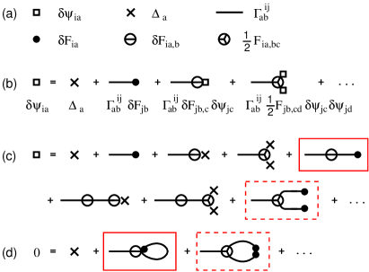
Figure 1: Diagrammatic expression of the perturbation scheme. (a) Definition of symbols. (b) Expression of Eqs.(10,11) and (c) its recursive expansion. (d) The ensemble average of (c). See text for interpretation of the framed graphs.

Now we take the average of Eq.(10) over the distribution of $\omega_{i}$’s. The LHS vanishes by the definition of $\delta\mbox{\boldmath$\psi$}$. On the RHS, $\delta F_{jb}$ and its derivative $\delta F_{jb,c}$ are averaged out unless they are correlated with a partner at the same site. Graphically, it means that the legs of the graphs (with the black dots at their ends) have to be attached to each other or to vertices to produce correlation terms. For example, the dot-framed graph in Fig.1(c) yields the corresponding graph in Fig.1(d), which reads $\Gamma_{ab}^{ij}\cdot\frac{1}{2}\left\langle F_{jb,cd}\right\rangle_{j}\cdot\Gamma_{ce}^{jk}\Gamma_{df}^{jk}\left\langle\delta F_{ke}\delta F_{kf}\right\rangle_{k}$, where $\left\langle\cdots\right\rangle_{j}$ means the average over the distribution $P(\omega_{j})$. Using the expansion (13) with the trace $G^{n}_{jj}=\sigma_{n}$, we obtain the $O(\epsilon^{2})$ expression of this graph as

$$\frac{\sigma_{2}}{2}f_{a,cd}\left(g_{cd}-f_{c}f_{d}\right),$$

where the functions $f_{a,cd}(\overline{\mbox{\boldmath$\psi$}})=\frac{\partial^{2}f_{a}}{\partial\psi_{c}\partial\psi_{d}}$ and $g_{ab}(\overline{\mbox{\boldmath$\psi$}})=\left\langle F_{ka}F_{kb}\right\rangle_{k}$ are introduced. Another graph that gives an $O(\epsilon^{2})$ contribution is framed by solid lines in Fig.1(d). It reads $\Gamma_{ab}^{ij}\Gamma_{cd}^{jj}\left\langle\delta F_{jb,c}\delta F_{jd}\right\rangle_{j}$ and is approximated as

$$\sigma_{2}f_{c,d}\left(h_{da,c}-f_{d}f_{a,c}\right)$$

with the function $h_{ab,c}(\overline{\mbox{\boldmath$\psi$}})=\left\langle F_{ja}F_{jb,c}\right\rangle_{j}$. We can see that these two graphs and $\Delta_{a}$ are the only $O(\epsilon^{2})$ contributions. Combining them and using Eq.(12), we obtain the self-consistent equation for $\overline{\mbox{\boldmath$\psi$}}$ to $O(\epsilon^{2})$ as

$$\overline{\psi}_{a} = f_{a}+\sigma_{2}(\delta_{ab}-f_{a,b})V_{b},$$ (14)

$$V_{b} = f_{c,d}\left(h_{db,c}-f_{d}f_{b,c}\right)+\frac{1}{2}f_{b,cd}\left(g_{cd}-f_{c}f_{d}\right).$$ (15)

Correlation Function.

The correlation function of the order parameter $C_{ab}^{ij}=C_{ab}({\bf r}_{i}-{\bf r}_{j})=\left\langle\delta\psi_{ia}\delta\psi_{jb}\right\rangle$ can be also computed using the diagrams. There is only one non-vanishing graph at $O(\epsilon^{2})$, which gives

$$C_{ab}^{ij}\simeq G^{2}_{ij}\left(g_{ab}-f_{a}f_{b}\right).$$ (16)

Note that $G^{2}_{ij}=G_{ik}G_{kj}$ is a function of ${\bf r}_{ij}={\bf r}_{i}-{\bf r}_{j}$. At large distance, it decays as $G^{2}_{ij}\propto|{\bf r}_{ij}|^{-d(1+2\epsilon)}$ for $\epsilon>0$, as we can see from a simple dimensional analysis. (For $d\geq 2$, $G^{2}_{ij}$ depends also on the direction of ${\bf r}_{ij}$ reflecting the lattice anisotropy). On the other hand, setting $i=j$ in (16), we obtain the variance of the order parameter,

$$\left\langle\delta\psi_{ia}\delta\psi_{ib}\right\rangle=\sigma_{2}\left(g_{ab}-f_{a}f_{b}\right).$$ (17)

Transition Behavior.

In order to solve the self-consistent equation (14,15), we need to compute $f_{a}$, $g_{ab}$, $h_{ab,c}$ and their derivatives as functions of $\overline{\psi}=\overline{\rho}e^{i\overline{\theta}}$. To simplify calculations, we choose the coordinate frame in which $\overline{\theta}=0$. Then the ensemble average of Eq.(8) gives

$$f_{a} = e_{a}(\overline{\rho})=\int_{-\infty}^{\infty}d\omega P(\omega)E_{a}(\overline{\rho},\omega)$$ (18)

$(a=R,I)$. Here, $E_{R}(\rho,\omega)$ and $E_{I}(\rho,\omega)$ are the real and imaginary parts of $E(\rho,\omega)$, respectively. Note that $f_{I}=e_{I}(\overline{\rho})=0$ thanks to the parity of $P(\omega)$ (even) and $E_{I}(\rho,\omega)$ (odd). The quadratic moments read

$$g_{RR} = e_{RR}(\overline{\rho}),\quad g_{RI}=g_{IR}=0,\quad g_{II}=e_{II}(\overline{\rho}),$$

$$e_{ab}(\overline{\rho}) = \int_{-\infty}^{\infty}d\omega P(\omega)E_{a}(\overline{\rho},\omega)E_{b}(\overline{\rho},\omega).$$ (19)

The calculations of the derivatives $f_{a,b}$, $f_{a,bc}$ and $h_{ab,c}$ are also straightforward. The non-vanishing components are found to be $f_{R,R}=e^{\prime}_{R},\,f_{I,I}=\widetilde{e}_{R},\,f_{R,RR}=e^{\prime\prime}_{R},\,f_{R,II}=f_{I,RI}=f_{I,IR}=\widetilde{e}_{R}^{\prime},\,$ and $h_{RR,R}=e^{\prime}_{RR}/{2},\,h_{RI,I}=\widetilde{e}_{RR},\,h_{IR,I}=-\widetilde{e}_{II},\,h_{II,R}=e^{\prime}_{II}/2,\,$ where ${}^{\prime}=d/d\rho$ and the abbreviations $\widetilde{e}_{R}=e_{R}/\overline{\rho}$, $\widetilde{e}_{RR}=e_{RR}/\overline{\rho}$, and $\widetilde{e}_{II}=e_{II}/\overline{\rho}$ are used. Substituting these into Eqs.(14,15), we obtain

$$\overline{\psi}_{R} = e_{R}+\sigma_{2}(1-e^{\prime}_{R})V_{R},\qquad$$ (20)

$$V_{R} = \frac{1}{2}\Big{[}e^{\prime}_{R}\left(e^{\prime}_{RR}-2e_{R}e^{\prime}_{R}\right)-2\widetilde{e}_{R}\widetilde{e}_{II}$$ (21)

$$\quad\qquad+\,e^{\prime\prime}_{R}\left(e_{RR}-e_{R}^{2}\right)+\widetilde{e}_{R}^{\prime}e_{II}\Big{]}.$$

and $\overline{\psi}_{I}=0$. On the RHS of (20) are functions of $\overline{\rho}$, which is related to $\overline{\psi}_{R}=\overline{\rho\cos\theta}$ on the LHS via the expansion $\overline{\rho}=\left\langle\sqrt{\psi_{R}^{2}+\psi_{I}^{2}}\right\rangle=\overline{\psi}_{R}+{\left\langle\delta\psi_{I}^{2}\right\rangle}/{\overline{\psi}_{R}}+O(\epsilon^{3}).$ Using this in the RHS of (20) with the result $\left\langle\delta\psi_{I}^{2}\right\rangle=\sigma_{2}e_{II}$ taken from Eq.(17), we arrive at the final form of the $O(\epsilon^{2})$ self-consistent equation,

$$\overline{\psi}_{R} = e_{R}+\sigma_{2}\left[(1-e^{\prime}_{R})V_{R}+e^{\prime}_{R}\widetilde{e}_{II}\right],$$ (22)

with the functions on the RHS evaluated at $\rho=\overline{\psi}_{R}$. Its solution gives the order parameter profile $\overline{\psi}_{R}=\overline{\psi}_{R}(\omega_{0})$. For $\sigma_{2}=0$, or $\alpha\leq d$, Eq.(22) reduces to the mean-field equation $\overline{\psi}_{R}=e_{R}(\overline{\psi}_{R})$ Kuramoto ; Kuramoto75 . The Taylor expansion $e_{R}(\rho)\approx(\omega_{c}/\omega_{0})(\rho-\rho^{3}/8)$ with $\omega_{c}=\sqrt{{\pi}/{8}}\simeq 0.627$ reproduces the global-coupling result that the order parameter vanishes for $\omega_{0}>\omega_{c}$. In contrast, for $\sigma_{2}>0$, or $\alpha>d$, there is no sharp transition, and the order parameter exhibits a long tail at large $\omega_{0}$, In fact, the approximation $e_{RR}(\rho)\approx e_{II}(\rho)\approx(8\omega_{c}/3\pi\omega_{0})\rho$ for $\rho\ll 1$ gives the asymptotic behavior of $\overline{\psi}_{R}$ for $\omega_{0}\gg\omega_{c}$,

$$\overline{\psi}_{R}\approx\frac{\sigma_{2}}{6\omega_{0}^{2}}.$$ (23)

The complete order parameter profile is obtained by numerical computation of the functions $e_{a}(\rho)$ and $e_{ab}(\rho)$, and is shown in Fig.2(a). Note that $\overline{\psi}_{R}$ in the current coordinate frame corresponds to $|\overline{\psi}|$ in the general frame. As we can see, the deviation from the mean-field profile is significant even for relatively small values of $\sigma_{2}$. (For comparison, $\sigma_{2}=0.2$ for $(d,\alpha)=(1,2)$ and $\sigma_{2}\simeq 0.057$ for $(d,\alpha)=(2,3)$ (square lattice).) The macroscopic order parameter is larger than the mean-field value for $\omega_{0}>\omega_{t}\simeq 0.504$, and smaller for $\omega_{0}<\omega_{t}$ for any non-zero value of $\sigma_{2}$. The enhancement of synchronization for large $\omega_{0}$ might look counter-intuitive, but it is a natural result of the spatial heterogeneity; there are regions that are more uniform than the others in terms of the intrinsic frequencies of the oscillators they contain. These regions can remain synchronized when the other regions are desynchronized, and contribute to the long tail of the order parameter profile. This effect of quenched heterogeneity is averaged out in the global-coupling case. Note also that we have rescaled the timescale so that $\sigma_{1}=1$. If $\sigma_{1}$ is not normalized, we must divide the intrinsic frequency and the order parameter by $\sigma_{1}$, which modifies Eq.(23) as $|\overline{\psi}|\approx{\sigma_{1}\sigma_{2}}/{6\omega_{0}^{2}}=Cg_{0}^{2}/\omega_{0}^{2}$, where $C$ is a function of $\alpha$ and $d$.

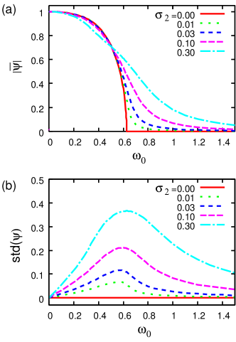
Figure 2: (a) The macroscopic order parameter $|\overline{\psi}|$ and (b) the standard deviation std$(\psi)=\left\langle|\delta\psi|^{2}\right\rangle^{1/2}$ as functions of $\omega_{0}$. The long tails scale as $|\overline{\psi}|\propto\sigma_{2}/\omega_{0}^{2}$ and std$(\psi)\propto\sigma_{2}/\omega_{0}$.

It should be briefly mentioned that the self-consistent solution bifurcates at very small $\omega_{0}$, into two stable branches $\overline{\psi}_{R1}\simeq 1$ and $\overline{\psi}_{R2}\ll 1$. The threshold $\omega_{b}$ rises with $\sigma_{2}$; e.g., $\omega_{b}=0.003$ for $\sigma_{2}=0.1$ and $\omega_{b}=0.022$ for $\sigma_{2}=0.3$. However, it turns out that the lower branch does not satisfy the condition for the series (13) to converge. It converges with its trace $\sum_{n=0}^{\infty}\sigma_{n}f^{n}_{a,a}$ if $\mbox{max}(e^{\prime}_{R}(\overline{\psi}_{R}),\tilde{e}_{R}(\overline{\psi}_{R}))<1/g_{0}$. Plotted in Fig.2(a) is the upper branch, which always meets the condition.

The standard deviation std$(\psi)=\left\langle|\delta\psi|^{2}\right\rangle^{1/2}$ is readily calculated from Eqs.(17,18,19), and is plotted in Fig.2(b). For any non-zero value of $\sigma_{2}$, it exhibits a peak near $\omega_{0}=\omega_{c}$ and a long-tail for $\omega_{0}\gg\omega_{c}$. The asymptotic behavior for large $\omega_{0}$ is obtained via the Taylor expansion of $e_{R}(\rho)$, $e_{RR}(\rho)$ and $e_{II}(\rho)$, as std$(\psi)\approx\sigma_{2}/3\sqrt{\omega_{c}}\omega_{0}$.

Summary.

We have found that the mean-field picture of sharp synchronization transition is valid only for $\alpha\leq d$, and the transition is broadened for $\alpha>d$. It could be regarded as a novel example of smeared transition in random systems, which usually requires spatially correlated disorder Vojta . The limitations of the perturbation theory for large $\alpha$ should be assessed by analysis of higher order corrections and comparison with numerical results, which are beyond the scope of the present paper and will be discussed elsewhere.

References

• (1) Y. Kuramoto, Chemical Oscillations, Waves, and Turbulence, (Springer, New York, 1984).
• (2) S. H. Strogatz, Physica D 143, 1 (2000).
• (3) J. A. AcebrΓ³n et al., Rev. Mod. Phys. 77, 137 (2005).
• (4) Y. Kuramoto, in Lecture Notes in Physics No. 30 (Springer, New York, 1975), p. 420.
• (5) J. D. Crawford and K. T. R. Davies, Physica D 125, 1 (1999).
• (6) H. Daido, Phys. Rev. Lett. 73, 760 (1994).
• (7) J. D. Crawford, 1995, Phys. Rev. Lett. 74, 4341 (1995).
• (8) H. Hong, H. ChatΓ©, H. Park and L.-H. Tang, Phys. Rev. Lett. 99, 184101 (2007).
• (9) H. Sakaguchi, S. Shinomoto and Y. Kuramoto, Prog. Theor. Phys. 77, 1005 (1987).
• (10) S. H. Strogatz and R. E. Mirollo, J. Phys. A 21, L699 (1988); Physica D 31, 143 (1988).
• (11) Y. Kuramoto, Prog. Theor. Phys. 94 321 (1995); Y. Kuramoto and D. Battogtokh, Nonlin. Phenom. Complex Syst. 5, 380 (2002).
• (12) D. M. Abrams and S. H. Strogatz, Phys. Rev. Lett. 93, 174102 (2004).
• (13) J. L. Rogers and L. T. Wille, Phys. Rev. E 54, R2193 (1996).
• (14) M. MarΓ³di, F. d’Ovidio, and T. Vicsek, Phys. Rev. E 66, 011109 (2002).
• (15) V. E. Tarasov and G. M. Zaslavsky, Chaos 16, 023110 (2006); N. Korabel, G. M. Zaslavsky and V. E. Tarasov, Commun. Nonlin. Sci. Numer. Simul. 12, 1405 (2007).
• (16) N. Uchida and R. Golestanian, Phys. Rev. Lett. 104, 178103 (2010).
• (17) N. Uchida and R. Golestanian, Europhys. Lett. 89, 50011 (2010).
• (18) T. Vojta, J. Phys. A: Math. Gen. 36, 10921-10935 (2003); Phys. Rev. E 70, 026108 (2004).