Critical behavior of hard-core lattice gases: Wang-Landau sampling with adaptive windows

Abstract

Critical properties of lattice gases with nearest-neighbor exclusion are investigated via the adaptive-window Wang-Landau algorithm on the square and simple cubic lattices, for which the model is known to exhibit an Ising-like phase transition. We study the particle density, order parameter, compressibility, Binder cumulant and susceptibility. Our results show that it is possible to estimate critical exponents using Wang-Landau sampling with adaptive windows. Finite-size-scaling analysis leads to results in fair agreement with exact values (in two dimensions) and numerical estimates (in three dimensions).

I Introduction

Recently efficient methods for estimating the number of configurations of classical statistical models have been developed. If the number $\breve{\Omega}(E)$ of configurations with energy $E$ is determined to sufficient accuracy, many thermodynamic quantities can be obtained with little further effort, for any desired temperature. Wang-Landau sampling (WLS) promises to be a simple and reliable approach for estimating $\breve{\Omega}(E)$ using Monte Carlo simulations landau ; landaupre . Critical exponents, the transition temperature (or chemical potential) and other quantities, such a cumulants, may then be estimated via finite size scaling (FSS) analysis fisher ; barber ; plichske ; binney . In this paper we test the Wang-Landau algorithm with adaptive windows adaptive_window , applying it to the lattice gas with nearest-neighbor exclusion.

Lattice gases have been used extensively as models of simple fluids, and along with the Ising model have received much attention in equilibrium statistical physics as a prototype for phase transitions. A particularly simple case is the lattice gas with nearest-neighbor exclusion (NNE), corresponding to an interparticle potential that is infinite for distances $\leq 1$ (in units of the lattice constant) and zero otherwise. In the absence of an energy scale, temperature is not a relevant parameter, and the system is termed athermal. It is known that on bipartite lattices, the lattice gas with NNE suffers a continuous phase transition between a disordered phase and an ordered one at a critical value of the density or of the reduced chemical potential $\mu\equiv\beta\widehat{\mu}$ gaunt ; runnels ; blote96 ; blote02 . ($\widehat{\mu}$ denotes the chemical potential.) In the ordered phase the occupation fractions of the two sublattices are unequal. The grand partition function is

$$\Xi(z,L)=\sum_{N=0}^{N_{max}}z^{N}\breve{\Omega}(N,L),$$ (1)

where $z=e^{\mu}$ is the fugacity, $N_{max}$ is the maximum possible number of particles, and $\breve{\Omega}(N,L)$ the number of distinct configurations with $N$ particles satisfying the NNE condition, under periodic boundaries. (On a hypercubic lattice of $L^{d}$ sites in $d$ dimensions, $N_{max}=L^{d}/2$ for $L$ even.) The order parameter is the difference between the occupations of sublattices A and B:

$$\phi=\frac{1}{N_{max}}\left\langle\left|\sum_{\bf x\in{\rm A}}\sigma_{\bf x}-\sum_{\bf x\in{\rm B}}\sigma_{\bf x}\right|\right\rangle,$$ (2)

where $\sigma_{\bf x}$ is the indicator variable for occupation of site x.

The NNE lattice gas has been studied on various structures: the square gaunt ; blote02 ; runnels , triangular zhang , simple cubic blote96 , hexagonal honeycomb , body-centered cubic bodycenter , and face-centered cubic lattices facecenter , and in higher dimensions luijten . Repulsive lattice gases with exclusion extending to second or further neighbors have also been studied runnels ; heitor . Various techniques have been applied to study the phase transition, including exact enumeration, series expansion (high- and low-density expansions), the cluster-variation method, transfer matrix analysis, and Monte Carlo simulation. The model exhibits Ising-like universality on the square and honeycomb lattices, while on the triangular lattice (Baxter’s hard-hexagon model baxter1 ; baxter2 ) it belongs to the three-state Potts model universality class.

In this paper we calculate the critical properties of the NNE lattice gas on the square and simple cubic lattices using the adaptive-window Wang-Landau (AWWL) algorithm, which has been shown to improve the performance of WLS adaptive_window ; polymer_cpc . The critical density and chemical potential, as well critical exponents and the reduced fourth-order cumulant, are estimated using FSS analysis. The balance of this paper is organized as follows. In Sec. II, the adaptive-window Wang-Landau algorithm is briefly reviewed. Sec. III contains our results for the number of configurations (exact enumeration and simulation results), thermodynamic quantities and critical exponents. A summary is provided in Sec. IV.

II Method

Consider a statistical model with a discrete configuration space, and let $\vartheta$ denote a variable (or set of variables) characterizing each configuration, such as energy or particle number. For a given system size, knowledge of the number $\breve{\Omega}(\vartheta)$ of configurations (called the “density of states”) for all allowed values of $\vartheta$ permits one to evaluate the partition function and associated thermal averages for arbitrary values of the temperature. Wang-Landau sampling (WLS) landau ; landaupre furnishes estimates of the configuration numbers, which we denote by $\Omega(\vartheta)$, reserving $\breve{\Omega}(\vartheta)$ to denote the exact values, which are in general unknown. This is done by performing a random walk in configuration space, with an acceptance probability proportional to $1/\Omega(\vartheta^{\prime})$, where $\vartheta^{\prime}$ denotes the values associated with the newly generated (or trial) configuration. In WLS one aims for equal numbers of visits to each set of allowed values of $\vartheta$, as reflected in the histogram, $H(\vartheta)$.

Various strategies have been proposed to improve WLS and optimize its convergence zhou_bhatt ; adaptive_window ; belardinelli1 ; belardinelli2 ; zhou . In this work we apply one such scheme, adaptive-windows WLS (AWWLS). This method estimates the density of states by determining the range over which the histogram has attained the desired degree of uniformity at various stages of the simulation.

The AWWLS procedure furnishes estimates, $\Omega(N;L)$, of the number of $N$-particle configurations on a lattice of $L^{d}$ sites, to within an overall multiplicative factor which is independent of $N$. For each accepted $N$-particle configuration, we update the histogram: $H(N)\to H(N)+1$. Since the density of states is not known a priori, we set $\Omega(N)=1$ for all $N$, at the beginning of each sampling level. In the simulation, if $N$ and $N+\Delta N$ are the particle numbers in the current and trial configurations, respectively, (in practice, $\Delta N=\pm 1$), then the acceptance probability is

$$p(N\rightarrow N+\Delta N)=\min\left[\frac{\Omega(N)}{\Omega(N+\Delta N)},1\right].$$ (3)

(To simplify the notation we suppress the dependence of $\Omega$ on system size $L$.)

Whenever a move to a configuration with $N$ particles is accepted, the density of states $\Omega(N)$ is updated, multiplying it by a modification factor $f>1$, so: $\Omega(N)\rightarrow f\cdot\Omega(N)$. If the trial configuration is rejected we update $\Omega(N)$ (as well as the histogram) of the current $N$ value. As is usual in WLS, the modification factor is initially set to $f_{0}=e=2.71828...$. After $m=10^{4}$ Monte Carlo steps we check if the histogram satisfies the flatness criterion on the minimal window, of width $W=(N_{max}-N_{min})/n$, beginning with $N_{min}$ note1 . The histogram is said to be flat if, for all levels in the window of interest, $H(N)>0.8\overline{H}$, where the overline denotes an average over levels within the proposed window. If it is not flat, we perform an additional $m$ Monte Carlo steps and check again, repeating until the histogram is flat on the minimal window. Once this condition is satisfied, we check whether the histogram is flat on a larger interval. Thus we define one window and repeat the procedure on the rest of the range of $N$ values, forming windows for each stage of sampling. The window positions depend on the portion of the histogram that is flat; we include an overlap of three levels between adjacent windows. This process is repeated until all values of $N$ have been included in a window with a flat histogram. Then a new stage is initiated: the modification factor is reduced, $f\rightarrow\sqrt{f}$, and we reset $H(N)=0$ for all $N$. This process is iterated and the simulation halted when $f-1$ is approximately $10^{-7}$. As explained in adaptive_window , window boundaries are not allowed to take the same positions on subsequent stages, to avoid distortions in $\Omega$ that arise when using fixed windows.

For simplicity, two kinds of trial moves are employed: insertion and removal of particles. Including particle-displacement moves - for which $N$ does not change - leads to the same results to within uncertainty. We use the R1279 shift register random number generator landau_binder_book .

III Results

We study the hard core lattice gas defined above using AWWLS. The estimates $\Omega(N)$ are used to calculate $\langle N\rangle$ and var$(N)$ directly; other thermal averages are given by

$$\left\langle A\right\rangle_{\mu}=\frac{\sum_{N}\left\langle A\right\rangle_{N}\Omega(N)e^{\mu N}}{\Xi}.$$ (4)

Here $\left\langle A\right\rangle_{N}$ is the microcanonical average of quantity $A$ over all configurations having exactly $N$ particles, which must also be estimated during the simulation. The development of reliable methods for estimating microcanonical averages is an important open problem pmoliveira . In the WL procedure, all configurations having the same $N$ should occur with the same probability, so that, in principle, the microcanonical average $\left\langle A\right\rangle_{N}$ should be taken over all accepted configurations having exactly $N$ particles, with equal weights. We nevertheless obtain better results if we restrict the microcanonical averages to the later stages of the sampling. Specifically, the averages $\left\langle\phi\right\rangle_{N}$, $\left\langle\phi^{2}\right\rangle_{N}$ and $\left\langle\phi^{4}\right\rangle_{N}$ calculated using all $N$-particle configurations accepted during the simulation yield estimates for critical exponents that deviate significantly from their expected Ising model values. Such deviations are not observed for systems with $L\lesssim 100$, but do appear for larger sizes. Similar problems were found in studies of spin models using WLS malakis2005 . The results for microcanonical averages improve when we restrict the sample to configurations accepted in the later stages of the simulation, i.e., for $f\lesssim 1+10^{-4}$.

III.1 Transfer-matrix analysis

As a preliminary test of our method, we compare our simulation estimates, $\Omega(N)$, with the results of an exact enumeration of $\breve{\Omega}(N)$, on a lattice of $8\times 8$ sites. The latter are obtained via a transfer matrix approach. One begins by enumerating the allowed configurations $\{c_{1},...,c_{\cal M}\}$ on a ring of $L$ sites, and storing the number $n(c_{j})$ of particles in each configuration. An ${\cal M}\times{\cal M}$ matrix ${\cal T}$ is then constructed, with ${\cal T}(c_{j},c_{j})=1$ if adjacent rings may assume configurations $c_{i}$ and $c_{j}$ without violating the NNE condition, and ${\cal T}(c_{i},c_{j})=0$ if the condition is violated. Then the allowed configurations on an $L\times L$ lattice with periodic boundaries are those sequences $\{c_{1},c_{2},...,c_{L}\}$ of ring configurations satisfying ${\cal T}(c_{1},c_{2}){\cal T}(c_{2},c_{3})\cdots{\cal T}(c_{L-1},c_{L}){\cal T}(c_{L},c_{1})=1$. The resulting numbers of configurations for $L=8$ are listed in Table 1.

To compare our simulation estimates against the exact enumeration, the former must be normalized, as simulation in fact provides $\Gamma(N)\equiv\alpha\Omega(N)$, with $\alpha$ an unknown constant, independent of $N$. To eliminate $\alpha$ we multiply the simulation estimates by a factor $\lambda$, varying $\lambda$ so as to minimize $\sum_{N}[\lambda\Gamma(N)-\breve{\Omega}(N)]^{2}$. This procedure is applied to each of the fifteen independent simulation studies, leading to the estimates and uncertainties listed in the Table. The relative error in estimating $\ln\breve{\Omega}$ is very small except near the minimum and maximum occupations. Even in the worst case, $N=N_{max}=32$, the relative error in $\ln{\breve{\Omega}}$ is $\approx 0.6\%$. If sampling errors were restricted to these regimes for larger system sizes, the effect on estimates for critical properties would be negligible.

$N$	$\breve{\Omega}(N)$	$\ln\breve{\Omega}(N)$	$\ln\Omega(N)$	$10^{3}\varepsilon(N)$
$0$	$1$	$0.0$	$0.010(14)$	$-$
$1$	$64$	$4.15888$	$4.163(11)$	$0.9989$
$2$	$1888$	$7.54327$	$7.543(10)$	$-0.0481$
$3$	$34112$	$10.43740$	$10.436(11)$	$-0.1701$
$4$	$423152$	$12.95549$	$12.954(11)$	$-0.1295$
$5$	$3830016$	$15.15838$	$15.158(9)$	$-0.0301$
$6$	$26249184$	$17.08315$	$17.086(9)$	$0.1501$
$7$	$139580160$	$18.75415$	$18.754(8)$	$-0.0003$
$8$	$585632520$	$20.18820$	$20.187(7)$	$-0.0515$
$9$	$1962132800$	$21.39730$	$21.396(7)$	$-0.0643$
$10$	$5296005568$	$22.39022$	$22.392(8)$	$0.0576$
$11$	$11591943552$	$23.17358$	$23.175(7)$	$0.0447$
$12$	$20681906352$	$23.75253$	$23.755(8)$	$0.1189$
$13$	$30206108416$	$24.13131$	$24.135(8)$	$0.1510$
$14$	$36251041536$	$24.31373$	$24.316(8)$	$0.0881$
$15$	$35886874048$	$24.30364$	$24.306(7)$	$0.0815$
$16$	$29436488660$	$24.10550$	$24.109(6)$	$0.1273$
$17$	$20127048512$	$23.72533$	$23.728(6)$	$0.1330$
$18$	$11573937440$	$23.17202$	$23.174(7)$	$0.0997$
$19$	$5674532608$	$22.45925$	$22.462(6)$	$0.1247$
$20$	$2420605568$	$21.60728$	$21.612(5)$	$0.2128$
$21$	$922331136$	$20.64241$	$20.646(6)$	$0.1918$
$22$	$322239232$	$19.59080$	$19.586(7)$	$-0.2539$
$23$	$104747904$	$18.46707$	$18.459(8)$	$-0.4439$
$24$	$31534744$	$17.26660$	$17.253(11)$	$-0.7674$
$25$	$8617024$	$15.96925$	$15.956(12)$	$-0.7995$
$26$	$2080576$	$14.54816$	$14.539(12)$	$-0.6443$
$27$	$430848$	$12.97351$	$12.973(12)$	$-0.0571$
$28$	$73840$	$11.20966$	$11.215(13)$	$0.4370$
$29$	$9984$	$9.20874$	$9.214(15)$	$0.5301$
$30$	$992$	$6.89972$	$6.900(15)$	$0.0983$
$31$	$64$	$4.15888$	$4.160(17)$	$0.2085$
$32$	$2$	$0.69315$	$0.689(19)$	$-6.359$

Table 1: Comparison with numerical results (L=8) for the density of states. The relative error is $\varepsilon(N)=(\ln\Omega(N)-\ln\breve{\Omega}(N))/\ln\breve{\Omega}(N)$.

III.2 Square lattice

In this work we study $18$ system sizes in the range $16\leq L\leq 256$ using AWWLS. Let $N^{*}(L)$ be the value of $N$ that maximizes $\Omega(N)$, and let $N_{c}(L)$ be the value of $N$ that maximizes the probability distribution $P(N)=\Omega(N)\exp[\mu_{c}N]$ at the critical point $\mu_{c}$. Preliminary studies on lattices with $L\leq 200$ reveal that $N^{*}\simeq 0.227L^{2}$, whereas $N_{c}\simeq 0.369L^{2}$, so that $N_{c}\gg N^{*}$. As a result, configurations with $N<N^{*}$ make a negligible contribution to thermal averages in the neighborhood of the critical point. To economize processor time we therefore restrict our high-statistics studies (which extend to $L=256$), to $N$ values between $N^{*}(L)$ and $N_{max}=L^{2}/2$. For $L=8$, a study with sampling restricted to $N\geq N^{*}=14$ yielded results of equal accuracy as those obtained using unrestricted sampling, when compared against exact enumeration.

The following observation suggests that a further economy of processor time could be realized in studies of the critical region. Let $P_{c}(N,L)=z_{c}^{N}\Omega(N,L)$ be the contribution to the grand canonical partition function due to the set of all $N$-particle configurations at the critical point, and let $P^{*}(L)=\max_{N}[P_{c}(N,L)]=P(N_{c})$. For $N$ values such that $P_{c}(N,L)/P^{*}(L)<10^{-50}$, say, the contribution to $\Xi$ and thermal averages is negligible. It therefore seems reasonable to restrict the sampling to the interval $[N_{1},N_{2}]$ of $N$ values such that $P_{c}(N,L)/P^{*}(L)\geq 10^{-50}$. In practice we use $N_{1}=[0.315L^{2}-131]$ and $N_{2}=[0.423L^{2}+129$], where the brackets denote the largest integer. For $L\leq 300$, the largest size considered, the resulting interval is small enough to be studied using WLS without windows. Surprisingly, restricting the sampling in this manner yields estimates for critical exponents that deviate significantly from their expected Ising model values (for example, we find $\gamma/\nu=2.02(5)$ on the square lattice). We conclude that restricted sampling distorts the estimates for the numbers of configurations, and adversely affects microcanonical averages.

We turn now to the results obtained using the sampling interval $[N^{*}(L),N_{max}(L)]$. Figure 1 shows the number of configurations versus density $\rho$; the very good data collapse confirms the expected scaling

$$\Omega(N,L)\simeq\exp\left[L^{d}g(\rho)\right]$$ (5)

The inset shows $N^{*}$ as a function of system size. Here and below all averages and uncertainties are obtained using fifteen independent runs.

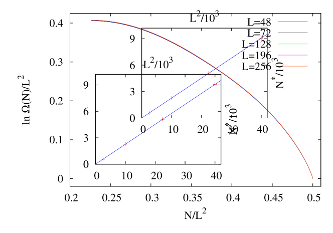
Figure 1: (Color online) Square lattice: $\ln\Omega/L^{2}$ versus density, system sizes as indicated. Inset: $N^{*}(L)$ versus system size.

Two thermodynamic properties used to characterize the transition in lattice gases are the particle density $\rho(\mu)$ and the compressibility,

$$\kappa(\mu)=\frac{L^{2}(\left\langle\rho^{2}\right\rangle_{\mu}-\left\langle\rho\right\rangle_{\mu}^{2})}{\left\langle\rho\right\rangle_{\mu}^{2}}.$$ (6)

Figure 2 shows simulation results for the density $\rho$ and compressibility $\kappa$ as functions of the chemical potential; Fig. 3 shows the order parameter, Eq. (2) and the susceptibility,

$$\chi(\mu)=L^{2}(\left\langle\phi^{2}\right\rangle_{\mu}-\left\langle\phi\right\rangle_{\mu}^{2}).$$ (7)

The insets in Fig. 3 show the data collapse obtained using the exact critical exponents, $\gamma/\nu=7/4$ and $\beta/\nu=1/8$, and the high-precision result for the critical chemical potential obtained by Guo and Blöte blote02 , $\mu_{c}=1.33401510027774(1)$.

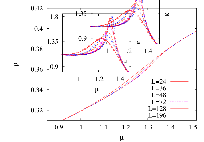
Figure 2: (Color online) Square lattice: density versus chemical potential on the square lattice. Error bars are smaller than the symbols. The inflection close to the transition point is weak, being imperceptible for the smaller systems. Inset: Compressibility versus chemical potential.

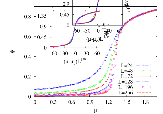
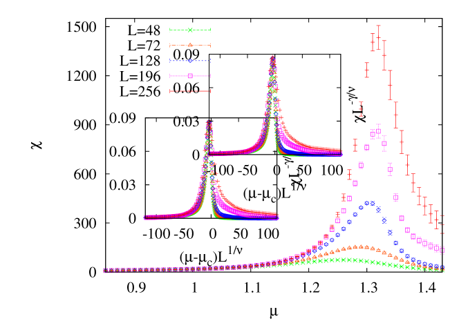
Figure 3: (Color online) Square lattice, upper panel: order parameter versus chemical potential. Lower panel: susceptibility versus chemical potential. The insets are data-collapse plots.

We analyzed the dimensionless ratio $Q_{4}=\left\langle\phi^{2}\right\rangle^{2}/\left\langle\phi^{4}\right\rangle$ (Fig. 4), related to Binder’s reduced cumulant binder_cum , which is expected to take a universal value at the critical point. Let $\mu_{c,L_{i}}$ denote the chemical potential at which $Q_{4}(L_{i})=Q_{4}(L_{i+1})\equiv Q_{c,L_{i}}$, i.e., the crossing between cumulants associated with a pair of successive systems sizes $L_{i}$ and $L_{i+1}$, and let $\overline{L}\equiv\sqrt{L_{i}L_{i+1}}$ denote the geometric mean of two successive sizes. It is common to plot $\mu_{c,L}$ and $Q_{c,L}$ versus $1/\overline{L}^{1/\nu}$ to estimate the critical chemical potential and cumulant, via extrapolation to $L\to\infty$. In the present case, however, we observe no tendency; all values of $Q_{c,L}$ and $\mu_{c,L}$ agree to within uncertainty. Averaging over all values we obtain $\mu_{c}=1.335(3)$ and $Q_{c}=0.852(6)$. Though of low precision, these results are consistent with the literature values quoted in Table 2.

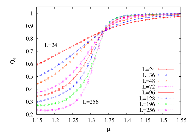
Figure 4: (Color online) Square lattice: fourth-order cumulant for system sizes as indicated.

Estimates for the critical chemical potential $\mu_{c}$ are obtained via analysis of the chemical potential values associated with the maxima of the susceptibility and compressibility for each system size. The extrapolated values, $\mu_{c}=1.330(1)$ using the susceptibility and $\mu_{c}=1.337(2)$ using the compressibility, are obtained using the susceptibility data for $L=20$ - $196$ and the compressibility data for $L=26$ - $196$. Pooling our results, we obtain $\mu_{c}=1.332(2)$. Linear extrapolation of the density $\rho(\mu_{c},L)$ versus $1/L$ yields $\rho_{c}=0.3675(5)$ (see Fig. 5), inset), consistent with the critical density reported in blote02 , $\rho_{c}=0.3677429990410(3)$. (Using the precise estimate for $\mu_{c}$ quoted above blote02 , we obtain $\rho_{c}=0.36800(5)$.)

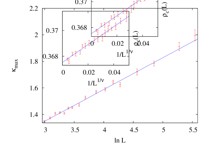
Figure 5: (Color online) Square lattice: maximum of the compressibility versus $\ln L$. The inset shows the density as a function of $1/L^{1/\nu}$.

Applying FSS analysis to the results for susceptibility for $L=22$ - $256$ yields $\gamma/\nu=1.764(7)$ (see the inset of Fig. 9). To estimate $\beta/\nu$ we analyze $\phi_{c}(L)$ using the above cited value of $\mu_{c}$ blote02 ; our data for $L\leq 256$ yield $\beta/\nu=0.123(2)$; (see Fig. 10 inset). (Using our own less accurate estimate, $\mu_{c}=1.332(2)$, we obtain $\beta/\nu=0.130(9)$.) Figure 5 shows the maximum of the compressibility versus system size; the results are consistent with $\kappa_{m,L}\sim\ln L$, as expected for a model in the 2d-Ising universality class. Table 2 summarizes our main results. It is interesting to note that we obtain essentially the same results, $\gamma/\nu=1.764(8)$, and $\beta/\nu=0.122(3)$, if we exclude the data for the two largest system sizes from the analysis.

	Present work	Literature values
$\mu_{c}$	$1.332(2)$	$1.33401510027774(1)$
$Q_{c}$	$0.852(6)$	$0.856$; $0.855(1)$; $0.85625(5)$
$\rho_{c}$	$0.3675(5)$	$0.3677429990410(3)$
$\gamma/\nu$	$1.762(8)$	$7/4$ (exact)
$\beta/\nu$	$0.123(2)$	$1/8$ (exact)

Table 2: Critical values for the square lattice obtained via WLS with adaptive windows. The results from nicolaides were obtained using Monte Carlo simulations while Refs. blote02 ; burkhardt ; kamieniarz use a transfer-matrix technique.

III.3 Cubic lattice

We apply AWWLS to the NNE lattice gas on the simple cubic lattice, in system sizes $L=8$, 10, 12, 14, 16, 18, 20, 22, 24, 28, 32, 40 and 48. In this case we sample the full range of $N$ values, using adaptive windows as described above; for $L=48$, we use approximately fifty windows. Figure 6 shows $\Omega(N)$, again verifying Eq. (5). The density and compressibility are plotted versus chemical potential in Fig. 7, while Fig. 8 shows the order parameter and susceptibility, and the inset of Fig. 6 the fourth-order cumulant.

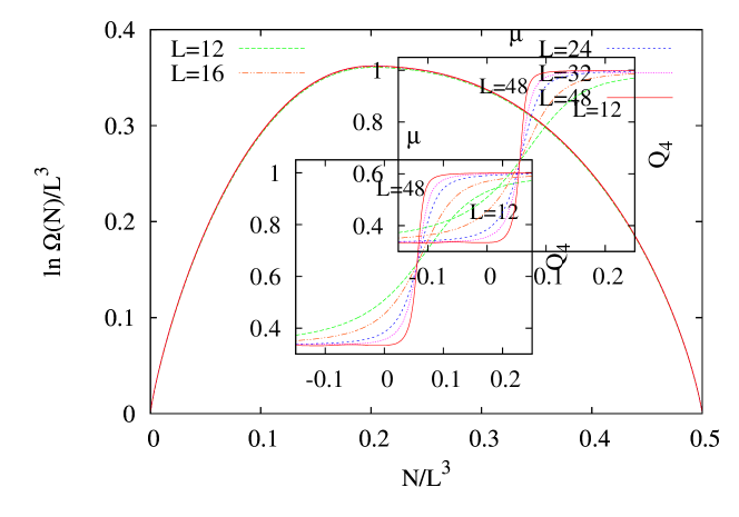
Figure 6: (Color online) Simple cubic lattice: $\Omega(N)$ versus density, system sizes as indicated. Inset: Fourth-order cumulant.

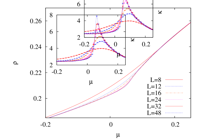
Figure 7: (Color online) Simple cubic lattice: density versus chemical potential. Inset: Compressibility versus chemical potential.

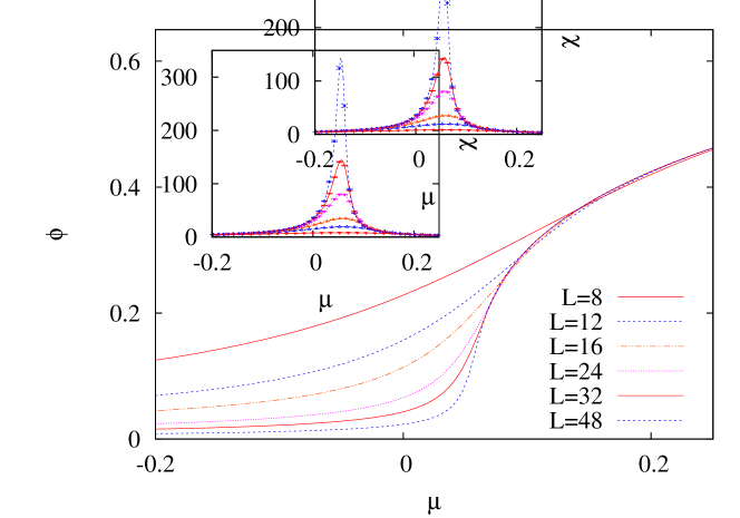
Figure 8: (Color online) Simple cubic lattice: Order parameter versus chemical potential. Inset: Susceptibility versus chemical potential.

Using the critical exponent $\nu=0.6301(4)$ pelissetto we plot the values $\mu_{c}(L)$ (corresponding to the maxima of the susceptibility and the compressibility) versus $1/L^{1/\nu}$. Extrapolation of the data for $L>14$ yields $\mu_{c}=0.05516(9)$ using the susceptibility, while the compressibility data (for $L>24$) yield $\mu_{c}=0.0567(2)$. (It is not surprising that the critical value obtained using the compressibility is less precise than that found using the susceptibility, as the former exhibits a weaker singularity than the latter.) Using our best estimate $\mu_{c}=0.05516(9)$ we calculate $\rho(\mu_{c},L)$; linear extrapolation (for $L>24$) versus $1/L^{1/\nu}$ yields $\rho_{c}=0.21082(5)$ (If we instead use the estimate $\mu_{c}=0.05443(7)$ blote96 , we find $\rho_{c}=0.21058(5)$).

Proceeding as in the case of the square lattice, we estimate the critical chemical potential $\mu_{c}$ and the critical moment ratio $Q_{c}$. Plotting $\mu_{c,L}$ against $1/\overline{L}^{1/\nu}$ we obtain $\mu_{c}=0.0552(7)$ via linear extrapolation. This is consistent with previous results blote96 which found $\mu_{c}=0.05443(7)$. Extrapolation of $Q_{c,L}$ as a function of $1/\overline{L}^{1/\nu}$ yields $Q_{c}=0.652(5)$, somewhat higher than the literature value (see Table 3). If we use $\mu_{c}=0.05443(7)$ blote96 to calculate $Q_{L}(\mu_{c})$, we observe no significant dependence on $L$; averaging over all values for $L>18$ yields $Q_{c}=0.636(3)$.

FSS analysis of the susceptibility furnishes $\gamma/\nu=2.056(6)$ (Fig. 9). Using $\mu_{c}=0.05443(7)$ blote96 , FSS analysis of the order parameter at $\mu_{c}$ yields $\beta/\nu=0.504(8)$ (Fig. 10). (Using our own best estimate, $\mu_{c}=0.05516(9)$, we find $\beta/\nu=0.477(7)$). Table 3 summarizes our principal results for the simple cubic lattice. As in the case of the square lattice, our results do not change significantly if we exclude the data for the two largest system sizes from the analysis.

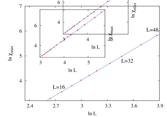
Figure 9: (Color online) Maximum of susceptibility versus system size on the square (inset) and simple cubic lattices. The solid lines are linear fits used to estimate $\gamma/\nu$.

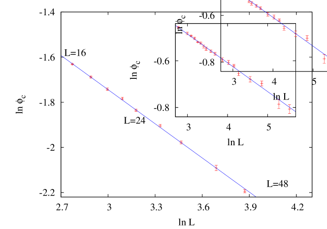
Figure 10: (Color online) Critical order parameter versus system size on square (inset) and simple cubic lattice. The solid lines are linear fits used to obtain $\beta/\nu$.

	Present work		Literature values
$\mu_{c}$	$0.05516(9)$	$0.05443(7)$	$-$	$-$
$Q_{c}$	$0.636(3)$	$0.626(4)$	$-$	$0.6233(4)$
$\rho_{c}$	$0.21082(5)$	$-$	$-$	$-$
$\gamma/\nu$	$2.056(6)$	$1.94(2)$	$2.005(6)$	$1.963(3)$
$\beta/\nu$	$0.504(8)$	$0.53(1)$	$0.5002(6)$	$0.519(2)$
$\alpha/\nu$	$0.25(1)$	$0.20(4)$	$-$	$0.174(4)$

Table 3: Critical values for the simple cubic lattice obtained via adaptive-window WLS. The results from blote96 were obtained using a cluster algorithm of the NNE lattice gas. Refs. garcia and blote95 are from high resolution cluster simulations of the Ising model.

III.4 Critical behavior of $g(\rho)$

As is known blote96 , the compressibility of the NNE lattice gas diverges as $\kappa\sim|\tilde{\mu}|^{-\alpha}$ in the vicinity of the critical point. (Here $\tilde{\mu}=(\mu-\mu_{c})/\mu_{c}$ is the reduced chemical potential.) On the other hand it is easy to show that $\kappa\propto 1/|g^{\prime\prime}(\rho)|$, where $g^{\prime\prime}$ denotes the second derivative of $g$ (defined in Eq. (5) with respect to $\rho$. Thus the singularity in the compressibility is reflected in a singularity in $g$. While plots of $g$ versus $\rho$ appear quite smooth (see Figs. 1 and 6), the second derivative does indeed exhibit a singularity near $\rho_{c}$. To obtain $g^{\prime\prime}$ we perform quadratic fits to $g(N)$ on windows of $b$ successive $N$ values. We choose $b$ large enough to eliminate small-scale fluctuations, but small enough that the singular behavior remains evident numbers . Despite the rounding incurred by such averaging (in addition, of course, to finite-size rounding), the data shown in Fig. 11 provide a clear indication of a developing singularity. The figure also shows that the minimum of $|g^{\prime\prime}|$ appears to approach zero as $L\to\infty$. Our data, however, are not sufficiently precise to verify the expected scaling, $|g_{min}^{\prime\prime}|\sim L^{-\alpha/\nu}$.

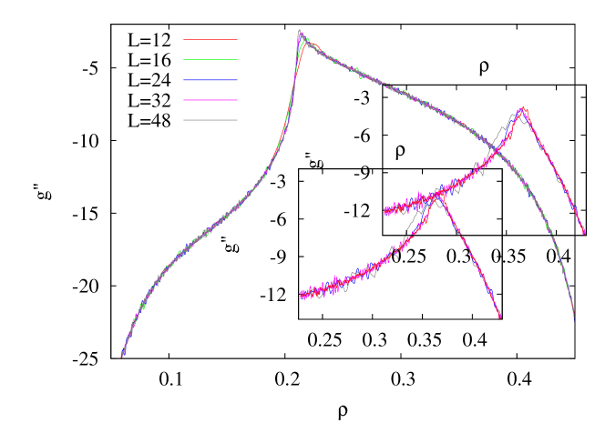
Figure 11: Second derivative of $g(\rho)$ on the simple cubic lattice, system sizes $L=12$, 16, 24, 32 and 48. The inset is a similar plot for the square lattice for system sizes $L=24$, 48, 128 and 196.

IV Conclusions

We perform adaptive-window Wang-Landau simulations of the lattice gas with nearest-neighbor exclusion on the square and simple cubic lattices. On the square lattice, comparison with an exact enumeration of configurations for $L=8$ yields excellent agreement. Using finite-size scaling analysis of data for systems of up $256^{2}$ sites on the square lattice and $48^{3}$ sites on the cubic lattice, we estimate the critical exponent ratios $\gamma/\nu$ and $\beta/\nu$, and the critical values of the chemical potential, the density, and the fourth cumulant. In general, fair agreement is observed with literature values. In three dimensions, the critical point is obtained with an error of about 1.3% compared with previous studies, and exponent ratios and $Q_{c}$ with an error of about 3.5%. The precision of our results is considerably less than that obtained using transfer-matrix or high-resolution Monte Carlo simulations. Although this is somewhat disappointing, we note that despite the widespread interest in Wang-Landau sampling, few studies have been published in which critical exponents are obtained via this technique malakis2004 ; malakis2005 ; malakis2008 ; malakis2009 ; malakis2010 . Our results confirm that it is possible to obtain reasonably accurate values for critical exponents and related quantities using Wang-Landau sampling with adaptive windows. It thus appears worthwhile to seek further improvements in the method, in efforts to develop a simple and versatile approach for studying phase transitions via Monte Carlo simulation.

In this regard two observations seem pertinent. The first is that restricting sampling to a subset of densities may worsen the results, even though densities outside this subset make a negligible contribution to thermal averages. It appears that the imposition of reflecting barriers on the random walk in configuration space somehow distorts the sampling. The second point is that the quality of the results furnished by the WLS procedure appears to decay with increasing system size, even while maintaining the same flatness criterion and schedule of updates of the factor $f$. Thus, including larger systems sizes in the analysis may not improve results; more extensive sampling of small and intermediate system sizes may represent a more effective allocation of computing resources. We hope to explore the reasons for, and implications of these observations in future work.

References

- (1) M. E. Fisher. Proceedings of the Enrico Fermi International School of Physics, Vol. 51, edited by M.S. Green (Academic Press, Varenna, Italy, 1971). M. E. Fisher and M. N. Barber, Phys. Rev. Lett. 28, 1516 (1972).
- (2) M. N. Barber, in Phase Transitions and Critical Phenomena, Vol. 8, edited by C. Domb and J. L. Lebowitz, (Academic Press, New York, 1983).
- (3) M. Plichske and B. Bergersen Equilibrium Statistical Physics (Cambridge University Press, Cambridge, 2008).
- (4) J. J. Binney, N. J. Dowrick, A. J. Fisher, M. E. J. Newman The Theory of Critical Phenomena: An Introduction to the Renormalization Group (Oxford University Press, Oxford, 2001).
- (5) F. Wang and D. P. Landau, Phys. Rev. Lett. 86, 2050 (2001).
- (6) F. Wang and D. P. Landau, Phys. Rev. E 64, 056101 (2001).
- (7) A. G. Cunha-Netto, A. A. Caparica, S.-H. Tsai, R. Dickman and D. P. Landau, Phys. Rev. E 78, 055701(R) (2008).
- (8) See, e.g., D. P. Landau and K. Binder, A Guide to Monte Carlo Simulation in Statistical Physics, 2nd Edition (Cambridge University Press, Cambridge, 2005).
- (9) T. D. Lee and C. N. Yang, Phys. Rev. 87, 410 (1952).
- (10) J. R. Heringa and H. W. J. Blöte, Physica A 232, 369 (1996).
- (11) W. Guo and H. W. J. Blöte, Phys. Rev. E 66, 046140 (2002).
- (12) D. S. Gaunt and M. E. Fisher, J. Chem. Phys. 43, 2840 (1965).
- (13) L. K. Runnels, Phys. Rev. Lett. 15, 581 (1965).
- (14) W. Zhang and Y. Deng, Phys. Rev. E 78, 031103 (2008).
- (15) L. K. Runnels, L.L. Combs, and J.P. Salvant, J. Chem. Phys. 47, 4015 (1967).
- (16) D. S. Gaunt, J. Chem. Phys. 46, 3237 (1967).
- (17) D. M. Burley, Proc. Phys. Soc. 75, 262 (1960).
- (18) J. R. Heringa, H. W. J. Blöte and E. Luijten, J. Phys. A: Math. Gen. 33 2929 (2000).
- (19) H. C. M. Fernandes, J. J. Arenzon and Y. Levin, J. Chem. Phys. 126, 114508 (2007).
- (20) R. J. Baxter, J. Phys. A 13, L61 (1980).
- (21) R. J. Baxter, Exactly Solved Models in Statistical Mechanics (Academic Press, San Diego, 1982).
- (22) C. Zhou and R. N. Bhatt, Phys. Rev. E 72, 025701(R) (2005).
- (23) R. E. Belardinelli and S. V. D. Pereyra, Phys. Rev. E 75, 046701 (2007).
- (24) R. E. Belardinelli and S. V. D. Pereyra, J. Chem. Phys. 127, 184105 (2007).
- (25) C. Zhou and J. Su, Phys. Rev. E 78, 046705 (2008) and references therein.
- (26) A. G. Cunha-Netto, R. Dickman and A. A. Caparica, Comput. Phys. Comm. 180, 583 (2009).
- (27) On the square lattice we use for , for , for between 100 and 196, and for . On the simple cubic lattice for , for , for between 24 and 32, and for .
- (28) P. M. C. de Oliveira, Braz. J. Phys. 30, 195 (2000).
- (29) K. Binder, Z. Phys. B 43, 119 (1981).
- (30) T. W. Burkhardt and B. Derrida, Phys. Rev. B 32 7273 1985.
- (31) D. Nicolaides and A. D. Bruce, J. Phys. A: Math. Gen. 21 223 (1988).
- (32) G. Kamieniarz and H. W. J. Blöte, J. Phys. A: Math. Gen. 26 201 (1993).
- (33) J. García and J. A. Gonzalo, Physica A 326, 464 (2003).
- (34) H. W. J. Blöte, E. Luijten and J. R. Heringa, J. Phys. A: Math. Gen. 28, 6289 (1995).
- (35) C. F. Baillie, R. Gupta, K. A. Hawick and G. S. Pawley, Phys. Rev. B 45, 10438 (1992).
- (36) A. Pelissetto and E. Vicari, Phys. Rep. 368 (2002) 549.
- (37) M. Kolesik and M. Suzuki, Physica A 215, 138 (1995).
- (38) B. G. Nickel, Physica A 177, 189 (1991).
- (39) B. G. Nickel and J. J. Rehr, J. Stat. Phys. 61, 1 (1990).
- (40) For the square lattice we use for , for , 20 for and 50 for ; for the simple cubic lattice, for and 16, for , 40 for and 70 for .
- (41) A. Malakis, A. Peratzakis, and N. G. Fytas, Phys. Rev. E 70, 066128 (2004).
- (42) A. Malakis, S. S. Martinos, I. A. Hadjiagapiou, N. G. Fytas, and P. Kalozoumis, Phys. Rev. E 72, 066120 (2005).
- (43) N. G. Fytas, A. Malakis, and I. Georgiou, J. Stat. Mech.: Theory Exp. L07001 (2008).
- (44) A. Malakis, A. N. Berker, I. A. Hadjiagapiou, and N. G. Fytas, Phys. Rev. E 79, 011125 (2009).
- (45) A. Malakis, A. N. Berker, I. A. Hadjiagapiou, N. G. Fytas, and T. Papakonstantinou, Phys. Rev. E 81, 041113 (2010).