Ultrafast sequential charge transfer in a double quantum dot

Abstract

We use optimal control theory to construct external electric fields which coherently transfer the electronic charge in a double quantum-dot system. Without truncation of the eigenstates we operate on desired superpositions of the states in order to prepare the system to a localized state and to coherently transfer the charge from one well to another. Within a fixed time interval, the optimal processes are shown to occur through several excited states. The obtained yields are generally between $99\,\%$ and $99.99\,\%$ depending on the field constraints, and they are not dramatically affected by strict frequency filters which make the fields (e.g., laser pulses) closer to experimental realism. Finally we demonstrate that our scheme provides simple access to hundreds of sequential processes in charge localization while preserving the high fidelity.

I Introduction

During the past few years, coherent control of charge in double quantum dots (DQDs) has been a subject of active experimental petta ; petta2 ; gorman ; kataoka and theoretical forre1 ; kosionis ; 2D_DQD ; salen ; nepstad ; fountoulakis research. Here one of the long-term aims is the design of a solid-state quantum computing scheme. loss It is still to be seen whether the optimal control mechanism DQDs turns out to operate through magnetic fields, popsueva ; harju gate voltages, kataoka or optimized laser pulses. 2D_DQD ; nepstad

Dynamical control of charge in DQDs has been a popular application for few-level schemes openov ; brandes ; grigorenko ; paspalakis ; voutsinas ; selsto ; kosionis ; fountoulakis (modeling DQDs as two-, three-, or four-level systems), which have demonstrated ultrafast high-fidelity processes. However, a physical DQD has, in principle, infinitely many levels, and in fast processes a considerable number of states might have practical relevance. For example, a two-level approximation is exact only in the limit of using an infinitely long resonant continuous wave with an infinitely small amplitude. A linear field (bias) is an appealing and simple alternative to control charge in DQDs, forre1 but it is not applicable to fast processes.

With quantum optimal control theory oct ; janreview (OCT) it is possible to find optimized external fields driving the system – having an arbitrary number of states – from the initial state to the desired target state without any approximations, apart from a possible model potential to describe the physical apparatus. OCT has been used to analyze the general controllability criteria of two-dimensional single-electron DQDs and to optimize interdot charge transfer. 2D_DQD Optimal control of two-electron DQDs has been obtained in an extensive work of Nepstad at al. nepstad addressing various control schemes degani and hyperfine interactions. hyperfine

In this work we apply OCT to construct external electric fields that lead to fast sequential charge transfer processes in single-electron DQDs. To obtain high fidelity we operate on the superpositions of the lowest states corresponding to the charge localization in left or right well. We show that hundreds of sequential charge transfer processes can be achieved without a significant loss of the yield. To make the experimental production of the obtained fields more realistic, we cut off the high-frequency components already during the optimization procedure. The use of such filters does not dramatically affect the fidelity.

II Model

We use a one-dimensional (1D) model describing a single-electron semiconductor DQD. The external potential has a form

$$V_{c}(x)=\frac{\omega_{0}^{2}}{2}\,\textrm{min}\Bigl{\{}\Bigl{(}x-\frac{d}{2}\Bigr{)}^{2},\Bigl{(}x+\frac{d}{2}\Bigr{)}^{2}\Bigr{\}}$$ (1)

in effective atomic units (a.u.), see below. Here $d=6$ is the interdot distance and $\omega_{0}=0.5$ is the confinement strength. The potential is visualized in Fig. 1.

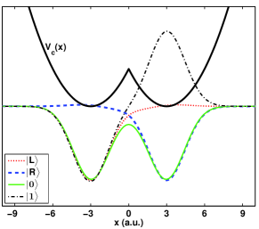
Figure 1: (Color online) Model potential for the quantum dot (black solid line), the ground state (green line), the first excited state (black dash-dotted line), and their superpositions corresponding to left (red dotted line) and right (blue dashed line) states.

We consider typical GaAs material parameters within the effective-mass approximation, i.e., $m^{*}=0.067$ and $\epsilon=12.7$. Now, the energies, lengths, and times scale as $E_{h}^{\ast}=(m^{\ast}/m_{0})/(\varepsilon/\varepsilon_{0})^{2}E_{h}\approx 11\,\mathrm{meV}$, $a_{0}^{\ast}=(\varepsilon/\varepsilon_{0})/(m^{\ast}/m_{0})a_{0}\approx 10\,\mathrm{nm}$, and $t_{0}^{\ast}=\hbar/E_{h}^{\ast}\approx 60\,\mathrm{fs}$, respectively. We emphasize that below the abbreviation a.u. refers to these effective atomic units.

It should be noted that a harmonic potential in Eq. (1) is, in its two-dimensional (2D) form, a general model for realistic semiconductor quantum-dot structures. qd_review Since the first Coulomb-blockade experiments it has been shown that the harmonic model is essentially valid up to dozens of electrons confined in the dot, and thus up to a large number of levels. The validity is clear, e.g., in recent works combining experiments and theory in the spin-blockade regime. spindroplet ; rogge The precise energy-level spectrum in a given device can be explicitly obtained through single-electron transport experiments, and this information can be utilized to reconstruct the particular form of the extenal potential. For example, in Ref. impurity, it was explicitly shown that measured energy-level spectrum can be well reproduced by a harmonic model potential upon slight refinements. Hence, when necessary, Eq. (1) can be tuned to match a particular device. Regarding the results below, the 1D model does not yield a qualitative difference from a more realistic 2D potential, but it significantly speeds up the calculations.

Electronic states localized to left and right dots can be expressed as superpositions of the two lowest (gerade and ungerade) states $\left.|0\right>$ and $\left.|1\right>$ as follows:

$$\left.|L\right> = \frac{1}{\sqrt{2}}(\left.|0\right>+\left.|1\right>)$$ (2)

$$\left.|R\right> = \frac{1}{\sqrt{2}}(\left.|0\right>-\left.|1\right>)$$ (3)

If the system is prepared in either of the superpositions, the occupation probabilities of $\left.|L\right>$ and $\left.|R\right>$ oscillate with the resonance frequency $\omega_{01}=E_{1}-E_{0}\approx 0.0135$ (see Ref. sakurai, ). For instance, if the system is first prepared at $\left.|L\right>$, it reaches the state $\left.|R\right>$ at $t=T/2=\pi/\omega_{01}\approx 232.87$. As discussed in detail below, we aim at controlling this charge-transfer procedure in an arbitrary way.

III Method

In OCT the objective is to find an external time-dependent field $\boldsymbol{\epsilon}(t)$ that drives the system into the predefined state through the solution of the Schrödinger equation,

$$i\frac{\partial}{\partial t}\Psi(\boldsymbol{r},t)=\hat{H}[\boldsymbol{\epsilon}_{k}(t)]\Psi(\boldsymbol{r},t).$$ (4)

Here $\boldsymbol{\epsilon}(t)$ is an electric field (e.g., laser pulse) dealt with the dipole approximation, so that the Hamiltonian has the form,

$$\hat{H}=\hat{T}+\hat{V}_{c}-\hat{\mu}\boldsymbol{\epsilon}(t),$$ (5)

where the (static) external potential is that of Eq. (1) where $\hat{\mu}=-{\mathbf{r}}$ is the dipole operator.

Starting with an initial guess for the electric field $\boldsymbol{\epsilon}(t)$, we maximize the expectation value of the target operator $\hat{O}$:

$$J_{1}[\psi]=\left<\Psi(\boldsymbol{r},T)|\hat{O}|\Psi(\boldsymbol{r},T)\right>,$$ (6)

where $\hat{O}=\left.|\Phi_{\rm F}\right>\left<\Phi_{\rm F}|\right.$ is now a projection operator, since we aim at maximizing the occupation of the target state $\Phi_{\rm F}$ at the end of the field at time $T$:

$$J_{1}=\left|\big{<}\Psi(\boldsymbol{r},T)|\Phi_{\rm F}\big{>}\right|^{2}.$$ (7)

In the following, this quantity is referred to the yield.

As a constraint, avoiding fields with very high energy, the fluence (time-integrated intensity) of the field is limited by a second functional,

$$J_{2}[\epsilon]=-\alpha\left[\int_{0}^{T}dt\,\epsilon^{2}(t)-E_{0}\right],$$ (8)

where $E_{0}$ is the fixed fluence [see Eq. (13) below] and $\alpha$ is a time-independent Lagrange multiplier. janreview

Finally, the satisfaction of the time-dependent Schrödinger equation [Eq. (4)] introduces yet another functional,

$$J_{3}[\epsilon,\Psi,\chi]=-2\,\textrm{Im}\int_{0}^{T}\big{<}\chi(t)|i\partial_{t}-\hat{H}(t)|\Psi(t)\big{>},$$ (9)

where $\chi(t)$ is a time-dependent Lagrange multiplier.

Variation of $J=J_{1}+J_{2}+J_{3}$ with respect to $\Psi$, $\chi$, $\epsilon$, and $\alpha$ lead to the control equations

$$i\partial_{t}\Psi(t) = \hat{H}(t)\Psi(t),\quad\Psi(0)=\Phi_{I},$$ (10)

$$i\partial_{t}\chi(t) = \hat{H}(t)\chi(t),\quad\chi(T)=\hat{O}\Psi(T),$$ (11)

$$\epsilon(t) = -\frac{1}{\alpha}\textrm{Im}\big{<}\chi(t)|\mu|\Psi(t)\big{>},$$ (12)

$$\int_{0}^{T}dt\,\epsilon^{2}(t) = E_{0}.$$ (13)

which can be solved iteratively. zhu ; janreview We apply a numerically efficient forward-backward propagation scheme introduced by Werschnik and Gross. Werschnik2 When solving the control equations, the Lagrange multiplier $\alpha$ is calculated through the fixed fluence $E_{0}$ as explained in detail in Ref. janreview, . The field is constrained by an envelope function of a form

$$f(t)=\frac{1}{2}\left\{\mbox{Erf}\left[\frac{a}{T}\left(t-\frac{T}{b}\right)\right]+\mbox{Erf}\left[-\frac{a}{T}\left(t-T+\frac{T}{b}\right)\right]\right\}$$ (14)

with $a=100$ and $b=20$. This corresponds to a step function ascending (descending) rapidly at $t\sim b/4$ ($t\sim T-b/4$). The scheme also allows straightforward inclusion of spectral constraints discussed in the following section. In the numerical calculations we have used the octopus code octopus which solves the control equations in real time on a real-space grid.

To approximate the time-propagator we applied the time-reversal symmetry, i.e., propagating $\Psi(t)$ forward by $\Delta t/2$ should correspond to propagating $\Psi(t+\Delta t)$ backward by $\Delta t/2$. This condition leads to an approximation for the propagator, evolution which can be further improved by extrapolating the time-dependent potentials. In octopus octopus the used method is called Approximated Enforced Time-Reversal Symmetry (AETRS).

IV Results

First, the system is prepared from the ground state $\left.|0\right>$ to the desired superposition. Hence, we simply define the target wave function in Eq. (6) as $\left.|\Phi_{\rm F}\right>=\left.|L\right>$. We set the field length to $T=100$ ($\sim 6$ ps) and the initial frequency to $0.5$ corresponding to the oscillator frequency $\omega_{0}$ of the DQD. Unless stated otherwise, the fluence is fixed to $E_{0}=0.3$, so that the average intensities are of the order of $10^{3}$ W/cm² (note the units given in Sec. II).

The optimized field in Fig. 1(a)

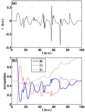
Figure 2: (Color online) (a) Optimized field to prepare the system to the superposition $\left.|L\right>$ (see text) from the ground state. (b) Occupations of the ground state $\left.|0\right>$, first excited state $\left.|1\right>$ and their superposition $\left.|L\right>$.

looks rather complicated with distinct high-frequency components, whose role and possible removal is discussed in detail below. The occupations of the states, i.e., their overlaps with the time-propagated wave function, are plotted in Fig. 1(b). The ground state (initially occupied) and the first excited state (initially empty) get half populated, so that their superposition $\left.|L\right>$ becomes fully populated and the electron is localized in the left well. The obtained yield is as high as $0.99985$.

After the preparation of the localized state we optimize a transition from $\left.|L\right>$ to $\left.|R\right>$, i.e., a charge transfer between the quantum wells. The result of the optimization is summarized in Fig. 3.

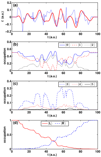
Figure 3: (Color online) (a) Optimized fields without (thin blue line) and with spectral constraints (thick red line) for transition $\left.|L\right>\rightarrow\left.|R\right>$. (b-c) Occupations of the five lowest eigenstates during the process. (d) Occupations of the initial and target superposition states.

The optimal field having a fixed duration of $T=100$ [thin blue line in Fig. 4(a)] leads to an extremely high yield of $0.9992$. In Fig. 3(b) and (c) we plot the occupations of the five lowest states during the charge-transfer process. Each of these states reach a maximum occupancy of more than $10\,\%$ during the process. The tenth lowest state still obtains $\sim 1\,\%$ of the occupation. Thus, with the present length of the field, the inclusion of several states seems to be crucial for the success of the optimization. Consequently, an alternative OCT procedure for a few-level model system (higher levels omitted) would lead to a completely different solution field, which most likely would perform poorly when applied to the “full” system (as here) due to the leaking of the occupancy to higher states. ringpaper

Similarly to the preparation field in Fig. 2(a), the optimized charge-transfer field in Fig. 4(a) shows abrupt peaks corresponding to high frequencies. Hence, the field would be practically impossible to construct, e.g., with the present pulse-shaping techniques. To relieve these limitations, we apply a spectral constraint cutting off the high-frequency components beyond a selected threshold frequency $\omega_{\rm th}$. The thick red line in Fig. 3(a) shows the field obtained using $\omega_{\rm th}=0.817$ ($\sim 14$ THz) in the optimization. The Fourier spectra of both fields are shown in Fig. 4(a).

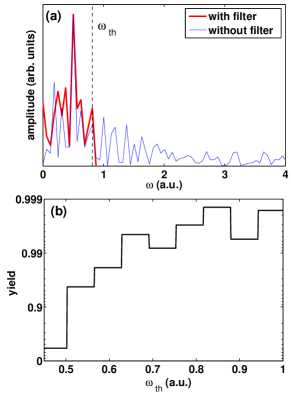
Figure 4: (Color online) (a) Spectrum of the optimized field for the process $\left.|L\right>\rightarrow\left.|R\right>$ without (blue thin line) and with a spectral constraint (red thick line) at $\omega_{\rm th}=0.817$. (b) Occupation of target state as the function of the frequency threshold $\omega_{\rm th}$ used as the filter. The step-like form of the curve is a consequence of the discrete Fourier transform.

Both fields have a peak at at $\omega=0.5$, which in fact corresponds to the oscillator frequency $\omega_{0}$ in Eq. (1).

It is interesting to note that despite the relatively strong frequency constraint at $\omega_{\rm th}=0.817$, leading to a considerable smaller search space for the optimization, the obtained yield is reduced only down to $0.9986$. This is a significant result in view of the fact that the original field has a large fraction of high frequencies as shown in Fig. 4(a). Nevertheless, using a frequency filter does not considerably reduce the importance of higher states in the optimization: in this particular case the fifth lowest state still gains a maximum occupancy of $\sim 10\,\%$. In any case, further tightening of the threshold to smaller values leads to decrease in the overlap as demonstrated in Fig. 4(b). The dependency is nonmonotonic due to numerical variation (note the logarithmic scale) and has a step structure resulting from the discrete Fourier transform. Below $\omega_{\rm th}\sim 0.5$ corresponding to the oscillator frequency the fidelity collapses from $96\,\%$ to $42\,\%$. If the fluence of the field is increased from $0.3$ to $1$, the critical threshold remains at $0.5$, at which the fidelity decreases from $92\,\%$ to $74\,\%$.

Besides the threshold frequency, the main constraints in the field to be optimized are the length and the fluence. In Fig. 5(a)

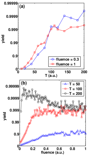
Figure 5: (Color online) (a) Obtained yield for the process $\left.|L\right>\rightarrow\left.|R\right>$ as a function of the field length. (b) Yield for the same process as a function of the fluence for three field lengths.

we show the yield, again for the process $\left.|L\right>\rightarrow\left.|R\right>$, as a function of the field length for fixed fluence values $E_{0}=0.3$ and $1$, respectively. Both cases show some saturation around $T\gtrsim 100$ although, as expected, the smaller fluence allows longer fields with even higher fidelities. However, increasing the yield above $0.9999$ is difficult in this fluence range unless relatively long fields are required. Here, the chosen length $T=100$ seems an appropriate compromise between $T$ and the obtained yield.

Figure 5(b) shows the yield as a function of the fluence for three fixed field lengths. We remind that the fluence is a time-integrated quantity [see Eq. (13)] so that the curves correspond to different distributions of the energy in the field. In all cases the yield first increases exponentially with the fluence until a point of saturation is reached. When $T=200$ the slight decrease in the overlap at fluences above $\sim 0.2$ might be due to numerical constraints: in that regime higher and higher states (with an increasing number of nodes) are required, and they have a finite accuracy on the numerical grid.

Finally we consider sequential charge-transfer processes by merging optimized fields together. For the process $\left.|L\right>\rightarrow\left.|R\right>\rightarrow\left.|L\right>\rightarrow\ldots$ we combine, in turns, the optimized field $\epsilon_{L\rightarrow R}$ (see above) with its time-inversion corresponding to $\epsilon_{R\rightarrow L}$. The combined field with a threshold frequency $\omega_{\rm th}=0.817$ is visualized in the upper panel of Fig. 6.

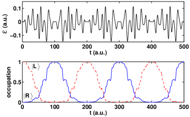
Figure 6: (Color online) Optimized field (upper panel) for the five-fold charge-switch process $\left.|L\right>\rightarrow\left.|R\right>\rightarrow\left.|L\right>...\rightarrow\left.|R\right>$ (lower panel) in a double quantum dot. Here we have used a threshold frequency of $\omega_{\rm th}=0.817$ leading to the target state occupation of $99.46\,\%$ at the end of the total five-fold process.

The lower panel shows the occupations of the states $\left.|R\right>$ and $\left.|L\right>$ by solid and dotted lines, respectively. The final yield after the five-fold process is $99.46\,\%$.

A more complete view on the results of up to 100 sequential processes is given in Table 1.

Table 1: Final-state occupations after $n$-fold sequential charge-switch processes obtained when merging the optimized fields. They are compared with an estimate based on the power of the yield given by the original (not inverted) field (see text).

$E_{0}$	$\omega_{th}$	$n=1$	$n=2$	$n=5$	$n=10$	$n=50$	$n=100$
$0.3$	$\infty$	0.9992(4)	0.9989	0.9975	0.9961	0.9848	0.9899
		power law	0.9985	0.9962	0.9924	0.9625	0.9263
$0.3$	$0.817$	0.9985(9)	0.9977	0.9946	0.9865	0.9562	0.9589
		power law	0.9972	0.9929	0.9859	0.9317	0.8681
$0.3$	$0.629$	0.9954(7)	0.9896	0.9606	0.8874	0.7092	0.7200
		power law	0.9910	0.9775	0.9556	0.7968	0.6349
$1.0$	$\infty$	0.9990(3)	0.9984	0.9964	0.9919	0.9952	0.9863
		power law	0.9981	0.9952	0.9903	0.9526	0.9074
$1.0$	$0.817$	0.9955(4)	0.9909	0.9842	0.9837	0.9838	0.9856
		power law	0.9911	0.9779	0.9563	0.7999	0.6398

We consider fluences $E_{0}=0.3$ and $1$ for a single process, respectively, and different threshold frequencies as well as the case without a filter, i.e., $\omega_{\rm th}\rightarrow\infty$. The total yield shown in the table can be expected to (roughly) follow a power law, $J_{1,\rm tot}=J_{1,\rm single}^{n}$, where $n$ is the number of processes (charge transfers). In this respect, the fidelity for a single transfer is essential for the quality of the final result. Indeed, the computational result follows the trend of the power law, but we find also significant differences: most importantly, in all cases the computational result is better than the prediction of the power law. The most dramatic discrepancy can be found in the last example with $E_{0}=1$ and $\omega_{\rm th}=0.817$, where after 100 pulses the yield is still almost $99\,\%$, whereas the power law predicts is only $64\,\%$. The reason behind the robustness of the yield in a sequential process is in the identity of the frequency components between the original and inverted fields, so that the population “lost” in higher states is partially attained back in the inverse process. There is, however, no clear trend in Table 1 indicating which field parameters are particularly favorable for robust sequential processes. Construction of such population-preserving, yet well optimized sequential fields is a subject of future work.

We point out that a critical aspect in the feasibility of the present approach is the sensitivity to decoherence. Typical decoherence mechanisms in semiconductor quantum dots are the hyperfine effects and interactions with optical and acoustic phonons. Their interplay and significance are largely dependent on the external conditions in a particular device. Detailed assessment of these mechanisms is beyond the scope of this work. We only mention that typical decoherence times in semiconductor quantum dots have been measured to be relatively large, even up to the millisecond scale, decoherence which in fact has been one of the main motivations of utilizing quantum dots in solid-state quantum computing. loss In view of the time scales considered here (up to hundreds of picoseconds) we believe that our approach is robust against the essential sources of decoherence, although further analysis is in order.

V Summary

Here we have numerically constructed optimal fields for charge-transfer processes in single-electron double quantum dots. The only approximation has been the model potential for the device, so that no truncation of eigenstates in terms of $N$-level approximations have been used. We have found that optimal control theory provides an efficient way to operate on desired superpositions of the eigenstates regarding both the preparation of the localized state as well as coherent charge transfer between the quantum wells. We have analyzed the interplay between different field constraints including the frequency filter, fluence, and the field length. Relatively strict frequency filters can be used without losing the extremely high yields obtained in the processes. Combination of the optimized pulses can be used in sequential charge transfers while preserving the high fidelity.

- (1) J. R. Petta, A. C. Johnson, C. M. Marcus, M. P. Hanson, and A. C. Gossard, Phys. Rev. Lett. 93, 186802 (2004).
- (2) J. R. Petta, A. C. Johnson, J. M. Taylor, E. A. Laird, A. Yacoby, M. D. Lukin, C. M. Marcus, M. P. Hanson, and A. C. Gossard, Science 309, 2180 (2005).
- (3) J. Gorman, D. G. Hasko, and D. A. Williams, Phys. Rev. Lett. 95, 090502 (2005).
- (4) M. Kataoka, M. R. Astley, A. L. Thorn, D. K. L. Oi, C. H. W. Barnes, C. J. B. Ford, D. Anderson, G. A. C. Jones, I. Farrer, D. A. Ritchie, and M. Pepper, Phys. Rev. Lett. 102, 156801 (2009).
- (5) M. Førre, J. P. Hansen, V. Popsueva, and A. Dubois, Phys. Rev. B 74, 165304 (2006).
- (6) S. G. Kosionis, A. F. Terzis, and E. Paspalakis, Phys. Rev. B 75, 193305 (2007).
- (7) E. Räsänen, A. Castro, J. Werschnik, A. Rubio, and E. K. U. Gross, Phys. Rev. B 77, 085324 (2008).
- (8) L. Sælen, R. Nepstad, I. Degani, and J. P. Hansen, Phys. Rev. Lett. 100, 046805 (2008).
- (9) R. Nepstad, L. Sælen, I. Degani, and J. P. Hansen, J. Phys.: Condens. Mat. 21, 215501 (2009).
- (10) A. Fountoulakis, A. F. Terzis, and E. Paspalakis, J. Appl. Phys. 106, 074305 (2009).
- (11) D. Loss and D. P. DiVincenzo, Phys. Rev. A 57, 120 (1998).
- (12) V. Popsueva, M. Førre, J. P. Hansen, and L. Kocbach, J. Phys.: Condens. Mat. 19, 196204 (2007).
- (13) J. Särkkä and A. Harju, Phys. Rev. B 80, 045323 (2009).
- (14) L. A. Openov, Phys. Rev. B 60, 8798 (1999).
- (15) T. Brandes and F. Renzoni, Phys. Rev. Lett. 85, 4148 (2000).
- (16) I. Grigorenko, O. Speer, and M. E. Garcia, Phys. Rev. B 65, 235309 (2002).
- (17) E. Paspalakis, Z. Kis, E. Voutsinas, and A. F. Terzis, Phys. Rev. B 69, 155316 (2004).
- (18) E. Voutsunas, A. F. Terzis, and E. Paspalakis, J. Mod. Opt. 51, 479 (2004).
- (19) S. Selstø and M. Førre, Phys. Rev. B 74, 195327 (2006).
- (20) A. P. Peirce, M. A. Dahleh, and H. Rabitz, Phys. Rev. A 37, 4950 (1988); R. Kosloff, S. A. Rice, P. Gaspard, S. Tersigni, and D. J. Tannor, Chem. Phys. 139, 201 (1989).
- (21) For a review, see, e.g., J. Werschnik and E. K. U. Gross, J. Phys. B: Atom. Mol. Opt. Phys. 40, R175 (2007).
- (22) I. Degani, A. Zanna, L. Sælen, and R. Nepstad, SIAM J Scient. Comp. 31, 3566 (2009).
- (23) R. Nepstad, L. Saelen, and J. P. Hansen, Phys. Rev. B 77, 125315 (2008).
- (24) For reviews, see L. P. Kouwenhoven, D. G. Austing, and S. Tarucha, Rep. Prog. Phys. 64, 701 (2001); S. M. Reimann and M. Manninen, Rev. Mod. Phys. 74, 1283 (2002).
- (25) E. Räsänen, H. Saarikoski, A. Harju, M. Ciorga, and A. S. Sachrajda, Phys. Rev. B 77, 041302(R) (2008).
- (26) M. C. Rogge, E. Räsänen, and R. J. Haug, Phys. Rev. Lett. 105, 046802 (2010).
- (27) E. Räsänen, J. Könemann, R. J. Haug, M. J. Puska, and R. M. Nieminen, Phys. Rev. B 70, 115308 (2004).
- (28) W. Zhu and H. Rabitz, J. Chem. Phys. 108, 1953 (1998); 109, 385 (1998).
- (29) J. Werschnik and E. K. U. Gross, J. Opt. B: Quantum Semiclass. Opt. 7, S300 (2005).
- (30) M. A. L. Marques, A. Castro, G. F. Bertsch and A. Rubio, Comp. Phys. Comm. 151, 60 (2003); A. Castro, H. Appel, M. Oliveira, C. A. Rozzi, X. Andrade, F. Lorenzen, M. A. L. Marques, E. K. U. Gross, and A. Rubio, Phys. Stat. Sol. (b) 243, 2465 (2006).
- (31) A. Castro and M. A. L. Marques, Lect. Notes Phys. 706, 197 (2006).
- (32) E. Räsänen, A. Castro, J. Werschnik, A. Rubio, and E. K. U. Gross, Phys. Rev. Lett. 98, 157404 (2007).
- (33) J. J. Sakurai, Modern Quantum Mechanics (Addison-Wesley, Reading, MA, 1994).
- (34) H. A. Engel, L. P. Kouwenhoven, D. Loss, and C. M. Marcus, Quantum Inf. Process. 3, 115 (2004).