Quenching of magnetic excitations in single adsorbates at surfaces: Mn on CuN/Cu(100)

Abstract

The lifetimes of spin excitations of Mn adsorbates on CuN/Cu(100) are computed from first-principles. The theory is based on a strong-coupling T-matrix approach that evaluates the decay of a spin excitation due to electron-hole pair creation. Using a previously developed theory [Phys. Rev. Lett. 103, 176601 (2009) and Phys. Rev. B 81, 165423 (2010)], we compute the excitation rates by a tunneling current for all the Mn spin states. A rate equation approach permits us to simulate the experimental results by Loth and co-workers [Nat. Phys. 6, 340 (2010)] for large tunnelling currents, taking into account the finite population of excited states. Our simulations give us insight into the spin dynamics, in particular in the way polarized electrons can reveal the existence of an excited state population. In addition, it reveals that the excitation process occurs in a way very different from the deexcitation one. Indeed, while excitation by tunnelling electrons proceeds via the s and p electrons of the adsorbate, deexcitation mainly involves the d electrons.

I Introduction

Recently, a series of experimental studies Hirjibehedin06 ; Hirjibehedin07 ; Tsukahara ; XiChen ; Iacovita ; Fu with low-temperature STM (Scanning Tunnelling Microscope) revealed that isolated adsorbates on a surface could exhibit a magnetic structure, i.e. that a local spin could be attributed to the adsorbate. Interaction of this local spin with its environment results in several magnetic energy levels that correspond to different orientations of the local spin relative to the substrate. A magnetic field, B, was also applied to the system: increasing the B field decouples the local spin from its environment and the system switches to a Zeeman structure, thus helping to characterize the adsorbate magnetic anisotropy. The energy of the various magnetic levels were obtained via a low-T IETS (low-Temperature Inelastic Electron Tunnelling Spectroscopy) experiment, in which the tip-adsorbate junction conductivity as a function of the STM bias exhibits steps at the magnetic excitation thresholds. The magnetic excitation energies are small, typically in the few meV range. Besides the spectroscopy properties, the IETS experiments also revealed that the conductance steps at the magnetic inelastic thresholds are very high, i.e. that the efficiency of the tunneling electrons in inducing magnetic transitions in the adsorbate is extremely large. In Metal-Phthalocyanine adsorbates for example Tsukahara ; XiChen , the tunneling current is dominated by its inelastic component when the bias is above the magnetic excitation thresholds. This efficiency is at variance with the efficiency of tunneling electrons in exciting vibrational modes in a molecular adsorbate which was observed and shown to only reach the few % range Ho ; Komeda ; Lorente00 . Several theoretical accounts of the magnetic excitation process have been reported based on perturbation theory Hirjibehedin07 ; Fransson ; Fernandez ; Persson , or on a strong coupling approach Lorente09 ; Gauyacq10 . In particular, the strong coupling approach quantitatively accounted for the very large efficiency of tunneling electrons in inducing magnetic transitions Lorente09 ; Gauyacq10 .

The existence on a surface of nano-magnets, the orientation of which could be changed at will by tunneling electrons, opens fascinating perspectives for the miniaturization of electronics. However, to lead to easily manageable devices, the excitation of local spins must have, among other properties, a sufficiently long lifetime. It is thus of paramount importance to know the decay rate of the excited levels of the local spin and in particular to decipher the various parameters and effects that govern its magnitude. Experimentally, the local spins were observed in systems in which a coating on the surface was separating the magnetic adsorbate carrying the local spin from the metal substrate. Experiments on adsorbates directly deposited on a metallic substrate did not lead to sharp IETS structures Balashov09 as the others and this was attributed to a too short lifetime of the magnetic excitation on metals, stressing the importance of the decoupling layer between local spin and substrate in stabilizing the magnetic excitation. Deexcitation of a local spin implies an energy transfer from the local spin to the substrate degrees of freedom, i.e. to the substrate electrons or to phonons. Phonons are not directly coupled to spin variables, but only via spin-orbit couplings (see e.g. a discussion in [Fabian99, ]). In contrast, the adsorbate spin variables can be directly coupled to substrate electrons and electrons colliding on a magnetic adsorbate can easily induce magnetic transitions. Actually, this is exactly what happens in the magnetic excitation induced by tunneling electrons in the IETS experiments described above; in the de-excitation process the tunneling electrons are simply replaced by substrate electrons. The decay of excited magnetic states in individual adsorbates thus proceeds via electron-hole pair creation. Substrate electrons colliding on the adsorbate can be thought to be as efficient in inducing magnetic transitions as tunneling electrons injected from an STM tip. In this qualitative view, one can expect the magnetic excitation decay rate to be the product of the collision rate of substrate electrons on the adsorbate by a very high efficiency factor.

Recently, the decay rate of excited magnetic Mn atoms adsorbed on CuN/Cu(100) has been measured by Loth et al Loth10 via the analysis of the dependence of the adsorbate conductivity on the tunneling current. The decay of the magnetic excitations was interpreted in the above scheme as a decay induced by collision with substrate electrons. The lifetimes of magnetic excitations were typically found to be of the order of a fraction of ns. In the present paper, we report on a theoretical ab initio study of the lifetime of magnetic excitations in the Mn/CuN/Cu(100) system using both a DFT-based (Density Functional Theory) description of the system and the strong coupling formalism Lorente09 ; Gauyacq10 developed to treat magnetic transitions induced by tunneling electrons; the corresponding results are compared with Loth et al data Loth10 .

II Method

II.1 Description of the magnetic deexcitation

The present treatment of the decay of magnetic excitations closely parallels our earlier treatment of magnetic excitations in IETS (see details in Ref. [Gauyacq10, ]). We assume that the magnetic levels of the adsorbate can be described by the following magnetic anisotropy Hamiltonian Yosida96 ,

$$H=g\mu_{B}\vec{B}\cdot\vec{S}+DS_{z}^{2}+E(S_{x}^{2}-S_{y}^{2}),$$ (1)

where $\vec{S}$ is the local spin of the adsorbate, $g$ the Landé factor and $\mu_{B}$ the Bohr magneton. $\vec{B}$ is an applied magnetic field. $D$ and $E$ are two energy constants describing the interaction of $\vec{S}$ with the substrate, i.e. the magnetic anisotropy of the system. Diagonalisation of Hamiltonian (1) yields the various states, $|\Phi_{i}\rangle$, of the local spin of Mn (we have used S=2.5, g=1.98, D=-41 $\mu$eV and E=7 $\mu$eV obtained in the experimental work Loth10 by adjustment to the magnetic excitation energy spectrum). For Mn on CuN, the local spin is 2.5 and there are thus 6 magnetic levels.

Figure 1 presents the energies $E_{i}$ of the anisotropy states, eigenstates of Hamiltonian (1) as a function of B, the applied magnetic field. Below, the ground state is noted ‘0’ and the excited states with i = 1-5. The easy axis of the system, the z-axis, is normal to the surface in this system. In the present study, coherently with the experimental study of Loth et al Loth10 , the B field has been put parallel to the surface, along the x-axis. As B is increased, the magnetic structure of the system changes from a magnetic anisotropy induced by the substrate with three doubly degenerate states at B=0 to the six states of a quasi-Zeeman structure at large B, where the $|\Phi_{i}\rangle$ states are eigenstates of $\vec{S}^{2}$ and $S_{x}$. The ground state at large finite B corresponds approximately to the $M_{x}=-2$ state. The energy diagram in Fig. 1 thus corresponds to the decoupling of the magnetic anisotropy by the B field. The structure appears a little complex at low B with several avoided crossings since the B field is not along the principal magnetic axis of the system.

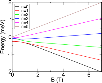
Figure 1: Energies of the six magnetic states in the Mn/CuN/Cu(100) system, eigenvalues of the magnetic anisotropy Hamiltonian  (1). They are presented as a function of the applied magnetic field, B, for a field along the x-direction.

The aim of the present work is to compute the decay of the excited states by collision with substrate electrons, i.e. by electron-hole pair creation. The decay rate, $\Gamma_{Tot,i}$, of an excited state, $|\Phi_{i}\rangle$, eigenstate of the Hamiltonian  (1) with energy $E_{i}$, is the inverse of its lifetime $\tau_{i}$ and it can then be written using matrix elements of the T transition matrix (we assume the energy variation of the T matrix to be small on the energy scale of the $i\rightarrow f$ transition and we assume a vanishing temperature of the substrate) Lorente08 ,

$$\frac{1}{\tau_{i}} = \Gamma_{Tot,i}=\sum_{f}\Gamma_{i,f}=\sum_{f}\frac{2\pi\delta\Omega_{f}}{\hbar}$$ (2)

$$\times \sum_{\begin{subarray}{c}k_{i},k_{f}\\ m_{i},m_{f}\end{subarray}}\left|\langle k_{f},m_{f},\Phi_{f}|\hat{T}|k_{i},m_{i},\Phi_{i}\rangle\right|^{2}$$

$$\times \delta(\varepsilon_{i}-\varepsilon_{f})\delta(\varepsilon_{i}-E_{F}),$$

where $|\Phi_{i}\rangle$ are the final states of the decay, associated to an energy transfer of $\delta\Omega_{f}=E_{i}-E_{f}$, and the total energy is $E_{T}=E_{i}+\varepsilon_{i}=E_{f}+\varepsilon_{f}$. The initial and final states of the substrate electrons are noted by their wave numbers, $k_{i}$ and $k_{f}$, and by their initial and final spin projections on the quantization axis, $m_{i}$ and $m_{f}$. The substrate is assumed to be non-magnetic. Each term, $\Gamma_{i,f}$, in the sum over $f$ is the partial decay rate of the initial state to a peculiar final state.

The electron-adsorbate collisions being very fast, we can treat them without the magnetic anisotropy (Hamiltonian  (1)) taken into account and later, include it in the sudden approximation. The electron-adsorbate collision is treated in a DFT-based approach (see section II.2 below) whereas the spin transitions are treated in the sudden approximation in a way similar to our earlier study of magnetic excitation Lorente09 ; Gauyacq10 . We thus define a collision amplitude for the substrate electrons independently of the magnetic anisotropy, it is a function of both the initial and final electron momenta, $k_{i}$ and $k_{f}$, and of the spin coupling between electron and adsorbate. The electron-adsorbate spin coupling scheme is defined via, $\vec{S}_{T}$, the total spin of the electron-adsorbate system: $\vec{S}_{T}=\vec{S}+\vec{s}$, where $\vec{S}$ is the adsorbate spin and $\vec{s}$ is the tunneling electron spin. The projection of $\vec{S}_{T}$ on the quantization axis is noted $M_{T}$. If the adsorbate spin is $S$, there are two collision channels corresponding to $S_{T}=S+\frac{1}{2}$ and $S_{T}=S-\frac{1}{2}$. The decay rate is then expressed as a function of the two channel amplitudes, $T^{S_{T}}$:

$$\frac{1}{\tau_{i}} = \sum_{f}\frac{2\pi\delta\Omega_{f}}{\hbar}\sum_{\begin{subarray}{c}k_{i},k_{f}\\ m_{i},m_{f}\end{subarray}}\left|\sum_{S_{T},M_{T}}\langle k_{f},m_{f},\Phi_{f}|S_{T},M_{T}\rangle T^{S_{T}}\langle S_{T},M_{T}|k_{i},m_{i},\Phi_{i}\rangle\right|^{2}\delta(\varepsilon_{i}-\varepsilon_{f})\delta(\varepsilon_{i}-E_{F}),$$ (3)

that can be re-expressed as:

$$\frac{1}{\tau_{i}} = \sum_{f}\frac{2\pi\delta\Omega_{f}}{\hbar}\sum_{\begin{subarray}{c}k_{i},k_{f}\\ m_{i},m_{f}\end{subarray}}\delta(\varepsilon_{i}-\varepsilon_{f})\delta(\varepsilon_{i}-E_{F})\left|\sum_{S_{T}}\langle k_{f}|T^{S_{T}}|k_{i}\rangle\sum_{M_{T}}\langle m_{f},\Phi_{f}|S_{T},M_{T}\rangle\langle S_{T},M_{T}|m_{i},\Phi_{i}\rangle\right|^{2}.$$ (4)

One can see that the contributions from the two $S_{T}$ terms are interfering. This corresponds to the a priori general case where no selection rule apply to the tunnelling process. In that case, the above expresion can be simplified by making an extra statistical approximation that neglects the interferences between the two $S_{T}$ channels. However, in our earlier studies on excitation processes Lorente09 ; Gauyacq10 it was found that one of the two $S_{T}$ channels was dominating the tunneling process between tip and adsorbate. Here for deexcitation in the Mn on CuN/Cu(100) system, only one $S_{T}$ coupling scheme does contribute significantly to the collision between substrate electrons and adsorbate (see Section II.2) and is thus included in the present treatment. One can note though that the dominating channel for the deexcitation process (collisions with electrons coming from the substrate) is different from that dominating the excitation (collision with tunnelling electrons) (see Section II.2).

If one considers a single $S_{T}$ channel, the decay rate can be rewritten as:

$$\frac{1}{\tau_{i}} = \sum_{f}\frac{2\pi\delta\Omega_{f}}{\hbar}\sum_{\begin{subarray}{c}k_{i},k_{f}\\ m_{i},m_{f}\end{subarray}}\delta(\varepsilon_{i}-\varepsilon_{f})\delta(\varepsilon_{i}-E_{F})\left|\langle k_{f}|T^{S_{T}}|k_{i}\rangle\right|^{2}\left|\sum_{M_{T}}\langle m_{f},\Phi_{f}|S_{T},M_{T}\rangle\langle S_{T},M_{T}|m_{i},\Phi_{i}\rangle\right|^{2}$$ (5)

$$= \sum_{f}\frac{2\pi\delta\Omega_{f}}{\hbar}\sum_{\begin{subarray}{c}k_{i},k_{f}\\ m_{i},m_{f}\end{subarray}}\delta(\varepsilon_{i}-\varepsilon_{f})\delta(\varepsilon_{i}-E_{F})\left|\langle k_{f}|T^{S_{T}}|k_{i}\rangle\right|^{2}P^{S_{T}}_{i,m_{i}\rightarrow f,m_{f}},$$

where $P^{S_{T}}_{i,m_{i}\rightarrow f,m_{f}}$ is a matrix element of spin variables only, corresponding to the $S_{T}$ coupling scheme for the $(i,m_{i}\rightarrow f,m_{f})$ transition. Equation (5) then becomes:

$$\frac{1}{\tau_{i}} = \sum_{f}\frac{2\pi\delta\Omega_{f}}{\hbar}\left(\sum_{k_{i},k_{f}}\delta(\varepsilon_{i}-\varepsilon_{f})\delta(\varepsilon_{i}-E_{F})\left|\langle k_{f}|T^{S_{T}}|k_{i}\rangle\right|^{2}\right)\left(\sum_{m_{i},m_{f}}P^{S_{T}}_{i,m_{i}\rightarrow f,m_{f}}\right)$$ (6)

$$= \sum_{f}\frac{2\pi\delta\Omega_{f}}{\hbar}T^{S_{T}}(E_{F})\left(\sum_{m_{i},m_{f}}P^{S_{T}}_{i,m_{i}\rightarrow f,m_{f}}\right)$$

The total and partial decay rates are then obtained via:

$$\frac{1}{\tau_{i}}=\sum_{f}\Gamma_{i,f}=\sum_{f}\frac{\delta\Omega_{f}}{h}(2\pi)^{2}T^{S_{T}}(E_{F})P_{Spin}(S_{T},i\rightarrow f).$$ (7)

Each partial decay rate thus appears as the product of a spin transition probability by the electron flux hitting the adsorbate in the energy range able to perform the studied transition.

As we will see below, the DFT-based calculation of the electron flux is not performed in the $S_{T}$, $M_{T}$ spin coupling base, but by specifying the scattering electron spin state (majority or minority). Thus we cannot perform a one to one identification. However, scattering through the adsorbate being dominated by a $S_{T}$ channel , we can identify the electron flux in the $S_{T}$ channel ($T^{S_{T}}(E_{F})$) with its equivalent in the DFT-approach, the total electron flux hitting the adsorbate $T^{Total}(E_{F})$. So that finally, the total decay rate is obtained as:

$$\frac{1}{\tau_{i}} = \Gamma_{Tot,i}$$ (8)

$$= \sum_{f}\Gamma_{i,f}=T^{Total}(E_{F})\sum_{f}\frac{\delta\Omega_{f}}{h}{P}_{Spin}(i\rightarrow f)$$

The decay rate is then equal to the total flux of substrate electrons hitting the adsorbate per second in the appropriate energy range, $T^{Total}(E_{F})\delta\Omega_{f}$, times a spin transition probability. Below, $T^{Total}(E_{F})$ is identified with the equivalent quantity computed in the DFT approach (Section II.2). One can stress the great similarity of this expression with that of the inelastic conductivity obtained in Ref. [Lorente09, ; Gauyacq10, ] as the total conductivity times a spin transition probability.

II.2 DFT-based calculation of the substrate electron collision rate

The quantity that we want to compute from first-principles simulations is,

$$T(E_{F})=(2\pi)^{2}\sum_{k_{i},k_{f}}\left|\langle k_{i}|\hat{T}|k_{f}\rangle\right|^{2}\delta(\varepsilon_{i}-\varepsilon_{f})\delta(\varepsilon_{i}-E_{F})$$ (9)

In this equation, $|k_{i}\rangle$ and $|k_{f}\rangle$ are asymptotic states that are solutions to the Hamiltonian sufficiently far away from a scattering center. In our case, the scattering center is the adsorbed atom. The goal is to calculate the amount of substrate (CuN/Cu(100) surface) electrons that scatter at the adsorbed Mn atom. From this quantity, we obtain $T^{Total}(E_{F})$ by summing the values for both spins,

$$T^{Total}(E_{F})=T(E_{F},\uparrow)+T(E_{F},\downarrow)$$ (10)

Following standard scattering theory formalism, we write the solutions to the full Hamiltonian (surface+adsorbed atom) as,

$$|\psi\rangle=|k_{i}\rangle+\hat{G}^{r}\hat{V}|k_{i}\rangle=|k_{i}\rangle+\hat{G}^{0r}\hat{V}|\psi\rangle$$ (11)

where $\hat{V}$ is the perturbation that couples the adsorbed atom and the substrate; and $\hat{G}^{r}$ and $\hat{G}^{0r}$ are the full system’s and unperturbed retarded Green’s functions, respectively. The $\hat{T}$ operator is then written as,

$$\hat{T}=\hat{V}+\hat{V}\hat{G}^{r}\hat{V}$$ (12)

In order to actually compute these vectors, matrices, and ultimately $T(E_{F})$, we have used the SIESTASiesta code, and a set of strictly localized atomic-like orbitals as a basis set. In terms of these, the Hamiltonian has the form,

$$\mathbf{H}=\left(\begin{array}[]{cc}\mathbf{H}_{SS}&\mathbf{H}_{SA}\\ \mathbf{H}_{AS}&\mathbf{H}_{AA}\end{array}\right)$$ (13)

where the $\mathbf{H}_{\mu\mu}$ are themselves matrices whose elements $H_{i,j}=\langle\phi_{i}|H^{DFT}|\phi_{j}\rangle$ are computed with orbitals centered around either surface (S) atoms or around the adsorbed atom (A). These orbitals are not orthogonal, $\langle\phi_{i}|\phi_{j}\rangle=S_{i,j}$. In this representation, the coefficients of the $|\psi\rangle$ and $|k_{i}\rangle$ states form a vector of components Deson_Transp ,

$$\mathbf{c}_{\psi}=\left(\begin{array}[]{c}\mathbf{c}_{S}\\ \mathbf{c}_{A}\end{array}\right)$$ (14)

$$\mathbf{c}_{k_{i}}=\left(\begin{array}[]{c}\mathbf{c}_{S}^{k_{i}}\\ 0\end{array}\right)$$ (15)

and the $|k_{i}\rangle$ are solutions to,

$$\left(\mathbf{H}_{0}-E\mathbf{S}_{0}\right)\mathbf{c}_{k_{i}}=0$$ (16)

$$\mathbf{H}_{0}=\left(\begin{array}[]{cc}\mathbf{H}_{SS}&0\\ 0&\mathbf{H}_{AA}\end{array}\right)$$ (17)

$$\mathbf{S}_{0}=\left(\begin{array}[]{cc}\mathbf{S}_{SS}&0\\ 0&\mathbf{S}_{AA}\end{array}\right)$$ (18)

The matrix version of equation (11) is,

$$\left(\begin{array}[]{c}\mathbf{c}_{S}\\ \mathbf{c}_{A}\end{array}\right)=\left(\begin{array}[]{c}\mathbf{c}_{S}^{k_{i}}\\ 0\end{array}\right)+ \left(\begin{array}[]{cc}\mathbf{G}^{r}_{SS}&\mathbf{G}^{r}_{SA}\\ \mathbf{G}^{r}_{AS}&\mathbf{G}^{r}_{AA}\end{array}\right)$$ (25)

$$\times \left(\begin{array}[]{cc}\mathbf{V}_{SS}&\mathbf{V}_{SA}\\ \mathbf{V}_{AS}&\mathbf{V}_{AA}\end{array}\right)\left(\begin{array}[]{c}\mathbf{c}_{S}^{k_{i}}\\ 0\end{array}\right)$$ (30)

and the Green’s functions matrices are defined as,

$$\mathbf{G}^{r}(E)=\left(E^{+}\mathbf{S}-\mathbf{H}\right)^{-1}$$ (31)

$$\mathbf{G}^{0r}(E)=\left(E^{+}\mathbf{S}_{0}-\mathbf{H}_{0}\right)^{-1}$$ (32)

$$E^{+}=\lim_{\delta\to 0}E+i\delta$$ (33)

What we need next, is to determine the perturbation matrix $\mathbf{V}$ entering equation (11). By multiplying equation (30) by $\left(E^{+}\mathbf{S}-\mathbf{H}\right)$ from the left, we get that $\mathbf{V}_{SS}=0$ and $\mathbf{V}_{AS}=\mathbf{H}_{AS}-E\mathbf{S}_{AS}$, where we have used equation (16) and the fact that,

$$\lim_{\delta\to 0}i\delta\mathbf{S}\mathbf{c}_{k_{i}}=0$$ (34)

Using the second part of equation (11) – the one that involves $\hat{G}^{0r}$ – in a matrix form equivalent to equation (30), we get that $\mathbf{V}_{AA}=0$. Imposing $\mathbf{V}$ to be hermitian, we finally have,

$$\mathbf{V}=\left(\begin{array}[]{cc}0&(\mathbf{H}_{SA}-E\mathbf{S}_{SA})\\ (\mathbf{H}_{AS}-E\mathbf{S}_{AS})&0\end{array}\right)$$ (35)

and we can see that $(\mathbf{H}_{0}+\mathbf{V}-E\mathbf{S}_{0})\mathbf{c}_{\psi}=0$. The energy-dependent form of $\mathbf{V}$ can be traced back to the the use of a non-orthogonal basis set Lang_GF ; Emberly_NonOrt .

The value of $\langle k_{i}|\hat{T}|k_{f}\rangle$ can thus be calculated with,

$$\langle k_{i}|\hat{T}|k_{f}\rangle = \left(\begin{array}[]{cc}\mathbf{c}^{k_{i}*}_{S}&0\end{array}\right).\left(\begin{array}[]{cc}\mathbf{T}_{SS}&\mathbf{T}_{SA}\\ \mathbf{T}_{AS}&\mathbf{T}_{AA}\end{array}\right).\left(\begin{array}[]{c}\mathbf{c}^{k_{f}}_{S}\\ 0\end{array}\right)$$

$$= \mathbf{c}^{k_{i}*}_{S}\mathbf{T}_{SS}\mathbf{c}^{k_{f}}_{S}$$

$$= \mathbf{c}^{k_{i}*}_{S}\left(\mathbf{V}_{SA}\mathbf{G}^{r}_{AA}\mathbf{V}_{AS}\right)\mathbf{c}^{k_{f}}_{S}$$ (42)

where we have used equation (12). Substituting this back into equation (9), we get that,

$$\frac{T(E_{F})}{(2\pi)^{2}} = \sum_{k_{i},k_{f}}\mathbf{c}^{k_{i}*}_{S}\left(\mathbf{V}_{SA}\mathbf{G}^{r}_{AA}\mathbf{V}_{AS}\right)\mathbf{c}^{k_{f}}_{S}\mathbf{c}^{k_{f}*}_{S}\left(\mathbf{V}_{SA}\mathbf{G}^{a}_{AA}\mathbf{V}_{AS}\right)\mathbf{c}^{k_{i}}_{S}\delta(\varepsilon_{i}-\varepsilon_{f})\delta(\varepsilon_{i}-E_{F}),$$ (43)

$$= Tr\left[\mathbf{V}_{AS}\left(\sum_{k_{i}}\mathbf{c}^{k_{i}}_{S}\mathbf{c}^{k_{i}*}_{S}\delta(\varepsilon_{i}-E_{F})\right)\mathbf{V}_{SA}\mathbf{G}^{r}_{AA}\mathbf{V}_{AS}\left(\sum_{k_{f}}\mathbf{c}^{k_{f}}_{S}\mathbf{c}^{k_{f}*}_{S}\delta(\varepsilon_{i}-\varepsilon_{f})\right)\mathbf{V}_{SA}\mathbf{G}^{a}_{AA}\right]$$

$$= \frac{1}{(2\pi)^{2}}Tr\left[\mathbf{\Gamma}_{AA}(E_{F})\mathbf{G}^{r}_{AA}(E_{F})\mathbf{\Gamma}_{AA}(\varepsilon_{i}=E_{F})\mathbf{G}^{a}_{AA}(E_{F})\right]$$

and we obtain the final expression for $T(E_{F})$,

$$T(E_{F})=Tr\left[\mathbf{\Gamma}_{AA}(E_{F})\mathbf{G}^{r}_{AA}(E_{F})\mathbf{\Gamma}_{AA}(E_{F})\mathbf{G}^{a}_{AA}(E_{F})\right]$$ (44)

In the derivation of equation (43) we have used that:

1. $\mathbf{c}^{j}_{S}\mathbf{c}^{j*}_{S}$ can be considered to define a matrix: $\mathbf{c}^{j}_{S}$ being a column vector, and $\mathbf{c}^{j*}_{S}$ a row vector.

2. The cyclic properties when taking the trace of a product of matrices.

3. The discontinuity of the retarded and advanced Green’s functions at the real axis Economou that in our basis set, considering item 1, gives,

   $$\sum_{j}\mathbf{c}^{j}_{S}\mathbf{c}^{j*}_{S}\delta(E-\varepsilon_{j})=\frac{i}{2\pi}(\mathbf{G}^{0r}_{SS}(E)-\mathbf{G}^{0a}_{SS}(E))$$ (45)

4. The self-energy and gamma matrices are written as Transiesta ,

   $$\mathbf{V}_{AS}\mathbf{G}^{0r(a)}_{SS}\mathbf{V}_{SA}=\mathbf{\Sigma}^{r(a)}_{AA}$$ (46)

   $$\mathbf{\Gamma}_{AA}=i\left[\mathbf{\Sigma}^{r}_{AA}-\mathbf{\Sigma}^{a}_{AA}\right]$$ (47)

We now describe the procedure to obtain $T(E_{F})$, defined in equation (44), from our ab-initio simulations. The ideas are the same as the ones used to derive the equations for the transmission function for electronic transport calculations, but since the final formulas are not exactly the same, we here include the derivation of the relations that we have used in the present work. To do so, we start by re-writing the DFT Hamiltonian (equation (13)),

$$\mathbf{H}=\left(\begin{array}[]{ccc}\mathbf{H}_{EE}&\mathbf{H}_{EC}&0\\ \mathbf{H}_{CE}&\mathbf{H}_{CC}&\mathbf{H}_{CA}\\ 0&\mathbf{H}_{AC}&\mathbf{H}_{AA}\end{array}\right)$$ (48)

where $\mathbf{H}_{EE}$ is a semi-infinite matrix describing the semi-infinite electrode (a region where the electronic structure, and matrix elements are assumed to be already bulk-like); and $\mathbf{H}_{CC}$ is the “slab” that describes the actual surface. The size of the $C$ (for contact) region is in principle arbitrary (but finite!), as long as it is thick enough to have: i) the $\mathbf{H}_{EA}$ ($\mathbf{H}_{AE}$) matrix elements equal to zero; and ii) the $\mathbf{H}_{EE}$ matrix elements sufficiently converged to bulk values.

For the purpose of simplifying the notation, let us define an $\mathbf{h}$ matrix to be,

$$\mathbf{h}=E\mathbf{S}-\mathbf{H}$$ (49)

To compute $T(E_{F})$, we need $\mathbf{G}^{r}_{AA}(E_{F})$ and $\mathbf{\Gamma}_{AA}(E_{F})$, where,

$$\mathbf{G}^{r}_{AA}=\left(\mathbf{h}_{AA}-\mathbf{\Sigma}_{AA}\right)$$ (50)

From Eqs. (46), (47) and (50), we can see that what we need is to compute $\mathbf{G}^{0r(a)}_{CC}$, the finite portion of $\mathbf{G}^{0r(a)}_{SS}$ needed to compute the self energies,

$$\mathbf{G}^{0r}_{CC}=\left(\mathbf{h}_{CC}-\mathbf{h}_{CE}\mathbf{G}^{0r}_{EE}\mathbf{h}_{EC}\right)$$ (51)

where it is important to note that only a finite number of elements of $\mathbf{h}_{CE}$ ($\mathbf{h}_{EC}$) have non-zero values, hence only a finite portion of $\mathbf{G}^{0r}_{EE}$ needs to be calculated. Since the $\mathbf{h}_{EE}$ matrix elements are assumed to be already “bulk-like”, the $\mathbf{G}^{0r}_{EE}$ matrix is obtained using the matrices extracted from a bulk calculation of the electrodeLopez_Algo ; Transiesta .

From these equations, we see that $T(E_{F})$ represents the flux of electrons coming from the substrate and scattering off the adsorbate back into the substrate. This quantity is different from the transmission function appearing in a Landauer-like approach Transiesta , where the adsorbate is connected to two electrodes. The difference is clear in the above equations, here a unique reservoir (the substrate) appears in the self-energies, and hence the decay appearing in the elastic Green’s function, Eq. (50), has only one self-energy instead of two in the transport case Transiesta .

III Density-functional study of a single Mn adsorbate on a CuN/Cu(100) surface

The ground-state electronic-structure configuration and the value for $T^{Total}(E_{F})$ were obtained by density-functional-theory (DFT) simulations. Our DFT calculations were performed using the SIESTA codeSiesta . The super cell contained at least six $4\times 4$ Cu (100) layers – a larger number of layers was used to test the convergence with respect to the size of the $C$ region, as discussed in section II.2; one CuN layer; and one Mn atom (see Fig. 2). The Mn atom and the two outermost layers were relaxed until the forces were smaller than 0.03 eV/Ang. A sampling of $3\times 3\times 1$ k-points was used. We have used the generalized gradient approximation PBE for the exchange-correlation potential.

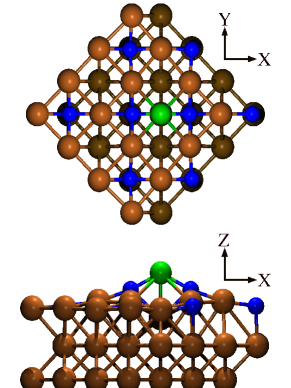
Figure 2: Top and lateral view of the geometry used to describe the Mn adsorbate (green) on top of a CuN/Cu(100) surface. The Mn atom is located on top of a Cu atom of the CuN layer, pushing it down while pulling up the N (blue) atoms close to it.

We have obtained a total spin polarization ($Q_{up}-Q_{down}$) of 4.7 Bohr magnetons, which essentially corresponds to a $S=\frac{5}{2}$ spin configuration, in good agreement with experiment Loth10 . The spin polarization is localized around the Mn atom, that has five half-filled d-orbitals, corresponding to five unpaired electrons. This can clearly be seen in Fig. 3.

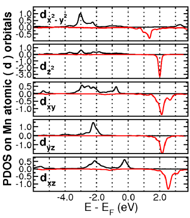
Figure 3: Projected density of states (PDOS) on the Mn atomic orbital for the case of Mn on CuN/Cu(100). For all the curves shown here, the positive (black) curves corresponds to the majority spin, and the negative (red) to the minority spin.

We now turn to the calculation of $T^{Total}(E_{F})$. As already discussed in section II.2, the thickness of the $C$ region of Eq. (48) is arbitrary (to some extent), and here we have taken the first three surface layers (including the CuN layer), as shown in Fig. 2. Since there is also some arbitrariness in the definition of what the atom is, we have considered different basis sets: from SZP to DZP, with larger and shorter cutoff radii. The differences in the results were not appreciable, and so here we report just the results for a DZP basis with large cutoff values — up to 10  Å  for the Mn basis orbitals.

We have computed T(E) for a range of energy values around the Fermi level, and the results are show in Fig. 4. As for $T^{Total}(E_{F})$, we have found $T^{Total}(E_{F})=T(E_{F},\uparrow)+T(E_{F},\downarrow)=0.8+0.3=1.1$. When we analyze the orbital contribution to the function T(E) of Fig. 4, we identify the d_xz orbital of Mn as responsible for the electron scattering off the Mn adsorbate. The above information on the characteristics of the substrate electrons hitting the adsorbate can be used to further specify the inputs of our spin-transition calculations. Indeed, the ground state of the system corresponds to putting one electron into each Mn d orbital (defined with the appropriate symmetry). This generates the $S=5/2$ $M=5/2$ state of the adsorbate. The dominant contribution to substrate electrons going through the adsorbate is found to involve the $d_{xz}$ orbital with majority spin as the transition intermediate; this is interpreted as a process involving a positive ion intermediate of $S_{T}=2$ symmetry. Similarly, the contribution associated to substrate electrons going through the $d_{xz}$ orbital with minority spin is interpreted as a process involving a negative ion intermediate of $S_{T}=2$ symmetry. So in all cases, the deexcitation process induced by substrate electrons going through the Mn adsorbate involves a $S_{T}=2$ intermediate and the associated electron flux is given by $T^{Total}(E_{F})=1.1$.

At this point, one can stress the stark contrast between the present deexcitation study and our earlier study on magnetic excitation by electron tunnelling between the tip and the substrate (Ref. [Lorente09, ]). In the tunnelling electron case, the Mn orbitals contributing to the transmission were the extended $s$ and $p$ orbitals whereas here, for the electrons scattering from the substrate into the substrate via the adsorbate, a $d$ orbital is dominating. In addition, the spin symmetry of the scattering intermediates are different : $S_{T}=2$ vs $S_{T}=3$. This study permits us to conclude that the de-excitation of spin states via electron-hole pairs takes place through the Mn $d$ electrons and in particular the d_xz orbital, while the spin excitation process proceeds via the tunneling electrons and are of $s$ and $p$ characters.

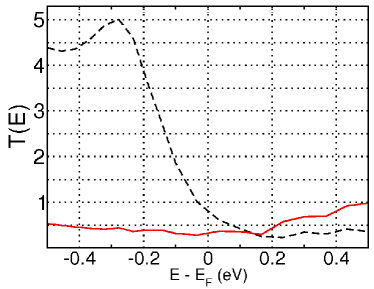
Figure 4: T(E) for the case of Mn on CuN/Cu(100). The black (dashed) curve corresponds to the majority spin, and the red (continuous) to the minority spin. $T^{Total}(E_{F})$ is the sum of T(E) for both spins at $E=E_{F}$. A sampling of $15\times 15$ k-points was used to obtain converged values for T(E).

IV Lifetime of the excited magnetic states

Equation (8) together with the results of section III has been used to compute the decay rates of the excited states of the system. Figure 5 presents the total decay rate, $\Gamma_{Tot,i}$, inverse of the lifetime, of the five excited states as a function of the applied magnetic field B. Two different regimes can be seen: low B and large B. At large B, the magnetic structure of the system is quasi-Zeeman. As a consequence, the decay of an excited state is dominated by one channel corresponding to a $\Delta M_{x}=-1$ selection rule. The B dependence of the decay rate is then that of the energy change associated to the decay, i.e. it is linear in B with a slope proportional to the dominant spin transition probability, $P_{Spin}$. At small B, the variation is more complex, reflecting the complex decoupling of the anisotropy by the B field on the x-axis (see Fig. 1). However, one can notice that the lowest excited state remains quasi-degenerate with the ground state almost up to 1T (Fig. 1), so that its decay rate is extremely small due to a quasi-vanishing $\delta\Omega_{f}$ (see Eq. (8)). Actually, this simply means that at low B, for a finite temperature, the two lowest states are roughly equally populated. As for the states 2-5, at low B, their decay rate is in the 2.0 $\mu eV$ range, corresponding to a lifetime of the order of 0.3 ns.

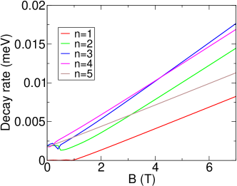
Figure 5: Decay rate (in meV) of the five excited magnetic states in the Mn/CuN/Cu(100) system as a function of the applied magnetic field B. The B field is along the x-axis. The decay rate is the inverse of the excited state lifetime.

One can stress that a different direction of the B-field leads to a different behaviour of the decay rates. The limit B = 0 is the same, obviously and the large B is almost independent of the B direction in the present case, but not completely due to an incomplete decoupling of the magnetic anisotropy for B = 7 T. The decay rates in the intermediate region, where the decoupling of the anisotropy occurs, depend of the direction of the B field with respect to the magnetic axis of the system.

Figure 6 presents a direct comparison between the present decay rate of the five excited states of Mn on CuN/Cu(100) and the decay rate extracted by Loth et al Loth10 from their experimental data. Two values of the magnetic field are presented: 3 and 7 T. For the sake of comparison, the experimental results of Loth et al have been multiplied by a global factor equal to 3.1. It appears that the present study reproduces extremely well the state dependence and the magnetic field dependence of the excited state lifetimes. However, the present results for the decay rates are a factor 3 larger than the experimentally extracted data. Besides inaccuracies and approximations in the experimental and theoretical procedures, one can invoke the sensitivity of the present results on the energy position of the $d_{xz}$ orbital in the calculations. Indeed, as we can see in Fig. 3 and 4, the electron flux hitting the adsorbate at Fermi level corresponds to the tail of the $d_{xz}$ majority and minority spin orbitals and any inaccuracy in the orbital energy directly affects, $T(E_{F})$, the electron flux.

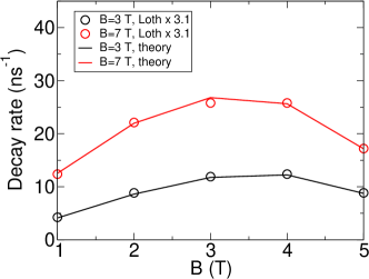
Figure 6: Comparison between the present decay rate (full lines) of the five excited magnetic states in the Mn/CuN/Cu(100) system with the experimental results of Loth et al Loth10 (symbols). The black symbols and line correspond to an applied B-field of 7T and the red symbols and line to 3T (the B-field is along the x-axis). For the sake of comparison, the experimental results of Loth et al have been multiplied by a global factor equal to 3.1.

V Modelling of the Mn junction conductance at large current

The experiments of Loth et al Loth10 introduce two main effects compared to the earlier ones in Ref.[Hirjibehedin06, ]. First, by using a polarized tip, these experiments introduce an unbalance between the spin up and spin down tunneling electrons that reveals the spin-dependence of the junction conductance. Second, they consider large currents flowing through the junction allowing a stationary population of excited states induced by the tunneling electrons. Indeed the two effects are linked together, tunneling electrons of different spins leading to different excited state populations. Below, we examine these two effects in the Mn on CuN/Cu(100) system allowing a modelling of the experimental situation.

V.1 Spin-dependence of the conductance of the adsorbed Mn atom

In references [Lorente09, ; Gauyacq10, ], we developed a strong coupling treatment of the elastic and inelastic tunneling of electrons through a magnetic adsorbate that inspired the above treatment of excited magnetic state decay. As explained in section  II, the magnetic anisotropy terms are small, and one can treat them in the sudden approximation and define a tunneling amplitude, independent of the magnetic anisotropy. As the main result (see details in [Gauyacq10, ]), the system conductance for the Mn atom in the magnetic state i, (in the case of only one $S_{T}$ symmetry contributing to tunneling) is given by:

$$\frac{dI}{dV}=C_{0}\frac{\sum_{n}\Theta(V-E_{n})\sum_{m,m^{\prime}}\left|\sum_{j}A_{j,i,m}A^{*}_{j,n,m^{\prime}}\right|^{2}}{\sum_{n}\sum_{m,m^{\prime}}\left|\sum_{j}A_{j,i,m}A^{*}_{j,n,m^{\prime}}\right|^{2}}$$ (52)

where $C_{0}$ is a global conductance; on the small energy range that we consider here and for a fixed tip-adsorbate distance, $C_{0}$ can be considered as constant. V is the junction bias and $E_{n}$ the energy of the various magnetic states, n, of the system. The $A_{j,n,m}$ coefficients are spin coupling coefficients giving the expansion of the eigenstates of $\vec{S}_{T}^{2}$ and $S_{T,z}$ on the initial or final states of the tunneling process, $|m,\phi_{n}\rangle$, (m refers to the tunneling electron spin state and $\phi_{n}$ is the magnetic anisotropy state of the adsorbate, eigenstate of the Hamiltonian (1)):

$$A_{j,n,m}=\langle S_{T},M_{T}|m,\phi_{n}\rangle\textit{, with }j=(S_{T},M_{T})$$ (53)

In both treatments (inelastic tunneling and excited state decay), the final result appears as a product of a magnetism-free quantity by a spin-coupling coefficient term, i.e. a global conductivity of the system is shared among the various anisotropy channels. The excitation probability is then only dependent on the weight of the incident and final channels in the intermediate tunneling intermediate and it can be very large. Such an efficient inelastic process has been invoked in several other processes involving angular momentum transfer (rotational or spin) in gas phase or surface problems Abram69 ; Teillet-Billy87 ; Bahrim94 ; Teillet-Billy00 , in all cases, it lead to high probabilities of inelastic scattering (see also a discussion in Ref. [Gauyacq10, ]). A change in the adsorbate-tip distance leads to a change in $C_{0}$ only and consequently in the tunneling current, but without a change in the excitation probabilities.

In the case of Mn on CuN/Cu(100), a DFT calculation showed that the $S_{T}$ = 3 symmetry is dominating the tunneling process Lorente09 and this accounted well for the observations of Hirjibehedin et al Hirjibehedin06 , obtained with non-polarised tunneling electrons. In Ref. [Lorente09, ; Gauyacq10, ], we only considered tunneling of non-polarised electrons, i.e. we summed the contributions from the two electron spin directions, both in the incident and final channels (the sum over $m$ and $m^{\prime}$ in equation (52)). Here we consider tunneling for a fixed direction of the electron spin (fixed $m$ or $m^{\prime}$) in the incident or final state (the spin directions are defined along the x-axis parallel to the applied B field). We thus use equation (52) with the sum over $m$ (or the sum over $m^{\prime}$) removed from the numerator. Figures 7 and 8 present the relative conductance of the various magnetic states of Mn for a fully polarized electrode and a B field of 3 T. Figure 8 corresponds for $V>0$ to an incident electron with an ’up’ spin and for $V<0$ to an electron in a final ’up’ state. Fig. 7 presents the ’down’ equivalent. In both cases the conductance is normalised in such a way that the conductance at $V=0$ for a non-polarised beam is equal to 1. The conductance presents steps at the magnetic excitation thresholds, due to the excitation induced by the tunneling electrons; the conductance also takes into account the possibility of de-excitation processes induced by the tunneling electrons, these present no energy thresholds. No broadening effect has been introduced in the conductance in Figs. 7,8,9 and the inelastic steps should be vertical; the finite slope visible in the figures comes from the finite number of V points that were actually computed.

Figure 7: Conductance of the various magnetic states in the Mn/CuN/Cu(100) system as a function of the tip bias in mV for a fully polarized electrode (spin down). The B-field is along the x-axis and is equal to 3T. The conductance has been normalized in such a way that the conductance for the ground state and a non-polarized tip is equal to 1 at zero bias.

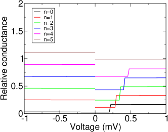
Figure 8: Conductance of the various magnetic states in the Mn/CuN/Cu(100) system as a function of the tip bias in mV for a fully polarized electrode (spin up). The B-field is along the x-axis and is equal to 3T. The conductance has been normalized in such a way that the conductance for the ground state and a non-polarized tip is equal to 1 at zero bias.

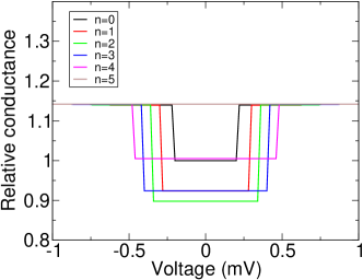
Figure 9: Conductance of the various magnetic states in the Mn/CuN/Cu(100) system as a function of the tip bias in mV for a non-polarized electrode. The B-field is along the x-axis and is equal to 3T. The conductance has been normalized in such a way that the conductance for the ground state and a non-polarized tip is equal to 1 at zero bias.

It appears that the conductances of the various anisotropy states for the two spin directions are quite different both in magnitude and shape (some have inelastic contributions and some do not). This is not surprising within our strong coupling approach: the magnitude of the conductivity is directly given by the weights of the initial and final channels (the $A_{j,n,m}$ coefficients) in the tunneling symmetry ($S_{T}=3$ in the present case) and these are strongly dependent on the considered initial and final states. One can also notice that the conductivity shown in figures 7 and 8 are discontinuous at $V=0$ (except for the ground state) due to the switch of definition at $V=0$ (spin selection for the initial state vs spin selection for the final state). The behaviour seen in 7 and 8 can be easily understood for the ’large’ B case depicted there. In that case, the anisotropy states are roughly Zeeman states, eigenstates of $S_{x}$ with the eigenvalues $M_{x}$. In that case, the increasing order of energy of the magnetic states corresponds to the increasing order of $M_{x}$ and the transitions induced by a tunneling electron verify the $\Delta M_{x}=\pm 1$ selection rule (the rule is strict only in the perfect Zeeman limit). As a consequence, excitation corresponds to a $\Delta M_{x}=+1$ selection rule and it can only exist for an incident ’up’ electron and an outgoing ‘down’ electron, and this appears clearly in Fig. 7 and 8, where the conductivity exhibits an inelastic step for only one sign of V, different for spins up and down. The inelastic steps appear as different energies for the different excited states, this is due to the fact that at 3 T the structure is not yet a perfect Zeeman structure (see Fig. 1), in this limit all inelastic steps would be at the same position given by $g\mu_{B}B$. Similarly, the very small excitation steps appearing at higher energy in addition to the $\Delta M_{x}=+1$ selection rule steps, as well as those appearing in the ’forbidden’ $V$ side, are due to the small difference from a pure Zeeman structure. The discontinuity in the conductance at $V=0$ is due to the existence of de-excitation processes induced by the tunneling electrons. Similarly to the excitation processes (well visible in Fig. 7 and 8), these are highly dependent on the sign of V, leading to a discontinuity at $V=0$. The purely elastic conductance is continuous at V = 0, as is the ground state conductance. Figure 10 shows a qualitative picture explaining this bias asymmetry.

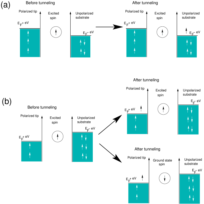
Figure 10: Qualitative scheme of the bias asymmetry in the tunneling process. For clarity of the illustration, we assume a $S=\frac{1}{2}$ adatom in its ‘spin-up’ state. The tip is completely polarized along the ‘up’ direction. (a) For positive bias, $V>0$, electron tunneling can only be elastic because the tip is spin polarized and aligned with the adatom’s spin. (b) For negative bias, $V\leq 0$, unpolarized electrons flow from the substrate and they can tunnel either elastically or inelastically. Hence, tunneling is different in cases (a) and (b) and so it presents a bias asymmetry due to the spin polarization of the tip.

Figure 9 presents the relative conductance for the various magnetic anisotropy states in the case of a non-polarised tip. Similarly to Fig. 7 and 8, the conductance has been normalised so that the conductance at $V=0$ for the ground state is equal to 1. All the conductivities are now continuous at $V=0$ and symmetric in V since no selection rule is imposed on the tunneling electron spin. The conductivity for each magnetic state exhibits a large inelastic step (except the highest lying state!) corresponding to the $\Delta M_{x}=\pm 1$ selection rule; much smaller excitation steps also appear at higher energies (barely visible in the figure) due to the non-perfect Zeeman structure. For all excited states, inelastic tunneling is significant compared to elastic tunneling, it is in the 15-25 % range, and different for the different states. One can also notice in Fig. 9 that the conductivities at large bias for all the states are equal, as a consequence of the summation over all possible excited states in Eq. 52. One can then conclude from Figs. 7-9 that the conductivity in the case of a polarised tunneling electron is quite different from that for a non-polarised one; in general, simply looking at majority and minority spins is insufficient, one has to resort to spin coupling arguments.

V.2 Description of the conductivity in the presence of excited states

The excitation of magnetic states by tunneling electrons is very efficient in the Mn/CuN/Cu(100). Though not as efficient as in some metal-phthalocynanine case Tsukahara ; XiChen ; Gauyacq10 , this can lead to a significant stationary population of excited states in an experiment with a finite current. This effect has been very clearly demonstrated by Loth et al Loth10 . We modelled this situation in a way very similar to that used by Loth et al Loth10 . The main difference lies in the absence of adjustment parameters in the present work: with the present treatment of the excitation process (section V.1) and of the decay process (sections II and IV), we can quantitatively predict the behaviour of the conductance as a function of the tunneling current.

The basic idea is to compute the stationary population of excited states that is induced by the tunneling current and then, via the excited conductance discussed in V.1, to get the junction conductivity. For an STM tip positioned above the Mn adsorbate, a tip bias V and a tunneling current I, the time dependence of the population, $P_{i}(I,V)$, of the magnetic state, i, is given by:

$$\frac{dP_{i}(I,V)}{dt}= - P_{i}(I,V)\left(\sum_{j}\Gamma_{i,j}+\sum_{j}F_{i,j}(I,V)\right)$$ (54)

$$+ \sum_{j}P_{j}(I,V)\left(F_{j,i}(I,V)+\Gamma_{j,i}\right)$$

where $\Gamma_{i,j}$ is the partial decay rate of state i towards state j (sections II and IV). $F_{i,j}(I,V)$ is the transition rate from state i to state j induced by the tunneling electrons (section V.1). It is given by:

$$F_{i,j}=CP_{Spin}(i,j)\Delta_{i,j}(V)$$ (55)

where $P_{Spin}(i,j)$ is the spin coupling coefficient of the considered $i\rightarrow j$ transition (section V.1) for the considered spin states of the tunneling electron. $\Delta_{i,j}(V)$ is an energetic factor; for the vanishing temperature considered here, it is equal to $V+E_{i}-E_{j}$ for an open excitation channel ($i\rightarrow j$ transition), to 0 for a closed excitation channel and to V for a de-excitation channel. C is a factor corresponding to the global conductance of the system. Below, the factor C is set so that the junction conductance at $V=0$, G, has a fixed value and then the whole spectrum of conductivity as a function of V is computed; changing C corresponds to moving the tip with respect to the Mn adsorbate i.e. to changing the magnitude of the tunneling current.

Equation (54) yields the time dependent population of the excited states, including the transient regime at the switching of the applied bias. The experiments being slow on the time scale of the excited state relaxation time (typically a fraction of ns, as seen in Fig. 5), the populations quickly reach stationary values which determine the observed conductivity. These stationary values are obtained by solving the homogeneous set of equations obtained from (54) by setting all time derivatives to zero. Once the populations are known the junction conductance is obtained by summing the contributions of the different states.

V.3 Population of the excited states

Loth et al Loth10 performed their experiments with a partial polarisation of the tip typically equal to $\eta=0.24$ so that the two spin directions of the electron have probabilities equal to 0.5 ($1\pm\eta$). In the present system, the ground state at large B is almost the $M_{x}=-\frac{5}{2}$ state. The polarisation of the tip is in the same direction, so that electrons with spin down are dominating at $V>0$ and holes with spin down at $V<0$.

The corresponding population of excited states for a junction conductance at $V=0$ equal to $2.10^{-6}$ S, a magnetic B field of 3 T and a tip polarisation equal to $\eta=0.24$ are shown in Fig. 11 as a function of V. Below the threshold for the $0\rightarrow 1$ transition, the population is entirely in the ground state, beyond this threshold the excited state population quickly increases as $|V|$ increases. One can notice that the excitation process at 3T basically goes step by step from state 0 to 5 following the energy (and index) order, so that excitation of the higher lying states is a multiple order process and rises much more slowly than excitation to state 1. At large $|V|$, the system reaches a regime where the population is independent of V, it corresponds to the situation where transitions (excitation and de-excitation) induced by tunneling electrons dominate over the excited state decay. Excitation by electrons and holes are very different leading to very different excited state populations in the $V>0$ and $V<0$ cases. ’Down’ polarised holes have a much higher excitation efficiency than ’down’ polarised electrons, and this is a direct consequence of the effects observed in Fig. 7 and 8 and discussed above. Actually, if we forget the very tiny excitations that correspond to the non-perfect Zeeman limit, a fully polarised tip would only lead to an excited state population for $V<0$ (see Fig. 7); here with a finite $\eta$ polarisation, the excited state populations at $V>0$ are due to the minority spin direction electrons in the tip. Indeed for a non-polarized tip, excitation by electrons and holes are equivalent, consistently with Fig. 9.

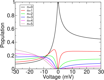
Figure 11: Population of the six magnetic states in the Mn/CuN/Cu(100) system as a function of the tip bias. The magnetic field is along the x-axis and equal to 3T. The tip polarisation, $\eta$, is equal to 0.24. The conductance at zero bias is equal to $2.10^{-6}$ S.

V.4 Modelling of Loth et al experiment

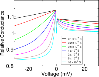
Figure 12: Relative conductance of the Mn/CuN/Cu(100) system as a function the tip bias. The tip polarization is $\eta=0.24$ and the B field, equal to 3T, is along the x-axis. The finite population of the excited states is taken into account. The various curves correspond to various absolute conductances at zero bias (0.1, 0.2, 0.5, 1., 2., 5. and 10. $10^{-6}$ S). In the figure, the conductance is plotted in relative value, with the conductance for zero bias set to 1.

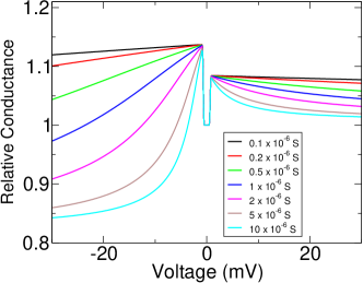
Figure 13: Relative conductance of the Mn/CuN/Cu(100) system as a function the tip bias. The tip polarization is $\eta=0.24$ and the B field, equal to 7T, is along the x-axis. The finite population of the excited states is taken into account. The various curves correspond to various absolute conductances at zero bias (0.1, 0.2, 0.5, 1., 2., 5. and 10. $10^{-6}$ S). In the figure, the conductance is plotted in relative value, with the conductance for zero bias set to 1.

Figures 12 and 13 present the conductivity of the Mn junction computed with a finite excited state population for different values of the conductance at $V=0:0.1,0.2,0.5,1.,2.,5.$ and $10.$ (all in $10^{-6}$ S). They correspond to a B field of 3 and 7 T, resp. and a tip polarisation of 0.24. The computed conductivity as a function of V has been convoluted with a Gaussian of 0.2 meV width to mimic the various broadening phenomena. Note that the actual height of the inelastic conductivity step for B = 3 T depends on the magnitude of the broadening effect, due to the small excitation energies (Fig. 1). The behaviour is the same as observed experimentally: i) there is a sharp peak at very low voltage corresponding to the excitation thresholds; ii) the conductivity drops as $|V|$ is increased due to the excited state population; iii) this drop is steeper and deeper on the $V<0$ side; iv) the steepness of the conductivity drop decreases as the tunneling current decreases to practically vanish for very small conductances and v) the conductance drop is steeper at 3T than at 7 T due to a longer lifetime of the excited states at 3T. The height of the inelastic steps and their asymmetry around zero, as well as the extent of the decrease of the conductance as $|V|$ increases depends on the polarisation of the tip. In the case of an unpolarised tip ($\eta=0$), Fig. 14 shows that, in the same way as for the experimental results, the conductivity is symmetric for $V>0$ and $V<0$ and it is practically independent of the tunneling current, although a significant population of excited states is present. Figure 15 shows the excited state population as a function of the junction bias for a conductivity of 2.0 $10^{-6}$ S at $V=0$ and for an unpolarized tip. For large bias, the excited state populations are large (their sum is larger than the population of the ground state); they are equal for positive and negative biases. Though no effect of these excited state populations is apparent in Fig. 14. This is a direct consequence of Fig. 9 where the conductances of all the magnetic states are equal above the excitation thresholds in the case of unpolarised electrons (or holes). Differences could only appear in the voltage region in between the inelastic thresholds, but in the present case, due to the smallness of the difference between the various excitation energy threshols, they are hidden by broadening effects. All these qualitative features nicely agree with the experimental observations. The two sets though differ quantitatively, coherently with the decay rate comparison in Fig. 6. The computed lifetimes are shorter and consequently, the effect of the excited state population on the junction conductivity appears for larger conductances and larger tunneling currents.

The effect of the populations of excited states on the polarized conductance is much visible in Figs. 12 and 13 which show the conductance as a function of bias for a fixed tip position. They also strongly emphasize a dependance of the conductance on the conductuctivity at $V=0$. One can stress that if all the curves in e.g. Fig. 12 are plotted as a function of the junction current $intensity$, then they look very much alike, the population of the excited states depending dominantly on the current intensity . In such a plot, the role of the bias voltage and conductivity at $V=0$ only appear in the excitation threshold region.

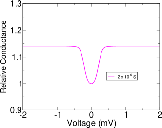
Figure 14: Relative conductance of the Mn/CuN/Cu(100) system as a function the tip bias. The tip is non-polarized and the B field, equal to 3T, is along the x-axis. The finite population of the excited states is taken into account. The conductance is independent of the current. In the figure, the conductance is plotted in relative value, with the conductance for zero bias set to 1.

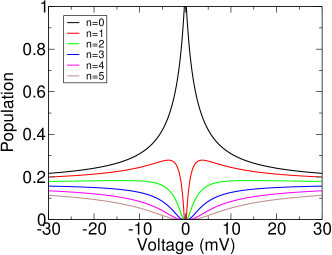
Figure 15: Population of the six magnetic states in the Mn/CuN/Cu(100) system as a function of the tip bias for a non-magnetic tip. The magnetic field is along the x-axis and equal to 3T. The conductance at zero bias is equal to $2.10^{-6}$ S. In contrast to Fig. 11, there is no bias asymetry.

V.5 Symmetry of the tunneling process

A very important feature in our strong coupling treatment of magnetic transitions is the symmetry of the tunneling state, i.e. which is the value of $S_{T}$ that is dominating tunneling through the adsorbate (see section V.1 above and a more detailed account in Ref. [Gauyacq10, ]). As shown by our DFT study in Ref.[Lorente09, ], the $S_{T}=3$ symmetry is dominating in the case of Mn/CuN/Cu(111). Different values of $S_{T}$ lead to different strengths of the magnetic transitions. For illustrative purpose, we checked the effect of changing the symmetry of the tunneling intermediate in the present study. Figure  16 shows the conductivity as a function of the STM bias, V, for a B field of 3T, a tip polarisation of $\eta=0.24$ and a conductance at $V=0$ of $2.10^{-6}$ S for three different tunneling symmetry hypothesis: i) $S_{T}=3$ dominating, ii) $S_{T}=2$ dominating and iii) both $S_{T}=3$ and 2 contributing in a statistical way. This change of symmetry only concerns the transitions induced by the tunneling electrons and not the excited state decay by electron-hole pair creation. Not surprisingly, the present physical situation with a partially polarised tip is highly sensitive to the symmetry of the tunneling intermediate. The three different symmetries are seen to lead to different qualitative behaviours: the heights of the inelastic steps at small $|V|$ are changing with the symmetry of the tunneling intermediate indicating a different efficiency of the various $S_{T}$ symmetries in the magnetic excitation process. In addition, depending on the symmetry and on the sign of $V$, the effect of excited state populations is seen to lead to an increase, a decrease or to a flat behaviour of the conductivity. Only the results for $S_{T}=3$ do exhibit the qualitative behaviour found experimentally. This comparison strongly supports our assignment of the $S_{T}=3$ symmetry as the dominant symmetry for the tunneling process in the present system. It also stresses the importance of considering the proper symmetry and proper spin coupling of the tunneling process for accounting for inelastic magnetic tunneling, especially with the present experimental protocol that involves a spin polarised tip and is thus much more selective.

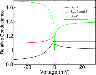
Figure 16: Relative conductance of the Mn/CuN/Cu(100) system as a function of the tip bias for various hypothesis in the spin-coupling scheme for the tunneling electrons ($S_{T}=3$ is the coupling scheme predicted by our DFT calculations). The tip polarization is $\eta=0.24$ and the B field, equal to 3 T, is along the x-axis. The absolute conductance is equal to $2.10^{-6}$ S for zero bias. In the figure, the conductance is plotted in relative value, with the conductance for zero bias set to 1. The finite population of the excited states is taken into account.

VI Concluding summary

We reported on a theoretical study of the lifetime of excited magnetic states on single Mn adsorbates on a CuN/Cu(100) surface. Electrons tunneling through a single adsorbate are very efficient in inducing magnetic transitions as was revealed by IETS experiments; similarly, substrate electrons colliding on adsorbates are also very efficient in quenching a magnetic excitation in a single adsorbate on a surface, the magnetic excitation energy being transferred into a substrate electron-hole pair. The present study on the quenching process is inspired by a recent study of magnetic excitations induced by tunneling electrons Lorente09 ; Gauyacq10 . It is based on a DFT calculation of the system associated to a strong coupling approach of the spin transitions. We show that the decay rate of an excited magnetic state can be written as the product of the flux of substrate electrons hitting the adsorbate by a spin transition probability. In the Mn/CuN/Cu(100) system, the lifetime of the excited states is found to be rather short, the calculated lifetimes are typically in the 0.04-0.4 ns range for an applied magnetic field in the 0-7 T range. The lifetime decreases when the B field rises.

For the comparison with Loth et al. experiments Loth10 , we performed a detailed study of electron tunneling through the adsorbed Mn atom in the case of a polarized tip. Using polarized electrons (or holes) unveils several phenomena among which we can stress:

• As shown in our strong coupling approach, the selection introduced by the symmetry of the total spin state in the tunneling process (total spin = spin of the tunneling electron + spin of the adsorbate) is very important and this leads to large differences in conductance between various situations: tunneling electrons (or holes) with spin up (or down), adsorbates in different magnetic states. All these can be related to the existence of a dominant spin symmetry in the tunneling process, which is $S_{T}=3$ in the case of Mn on CuN/Cu(100) as shown here.

• As the excitation probability by tunneling electrons is large, significant populations of excited states can exist for a finite current. Very interestingly, this leads to observable changes in the conductance as a function of current in the case of a polarized tip but not in the case of a non-polarized tip. This is a direct consequence of one of the key properties of the magnetic excitation process, as described in the strong coupling approach. The excitation process appears as a sharing process: a global tunneling current is shared among the various magnetic states, using sharing probabilities obtained from spin coupling coefficients. If we sum over all possible spin directions for the tunneling electron, these spin coupling coefficients sum to one. Thus, with a non-polarized tip, the conductance for biases above all inelastic thresholds is independent of the initial state and then independent of a finite stationary population of excited states. In contrast, in the case of a polarized tip, the sum over electron spin directions is not complete and the conductance depends significantly on the magnetic state.

• The present theoretical results reproduce all the behaviours observed experimentally, basically those are consequences of the two phenomena described above. Quantitatively, although the excitation process is perfectly accounted for, the computed lifetimes of the excited states appear to be a factor 3 shorter than those extracted from experiment. As a consequence, the experimentally observed variation of the junction conductivity with the tunnelling current is reproduced but for larger tunnelling currents.

- (1) C. F. Hirjibehedin, C. P. Lutz and A. J. Heinrich, Science 312, 1021 (2006).
- (2) C. F. Hirjibehedin, C.-Y. Lin, A. F. Otte, M. Ternes, C. P. Lutz, B. A. Jones and A. J. Heinrich, Science 317, 1199 (2007).
- (3) N. Tsukahara, K. Noto, M. Ohara, S. Shiraki, N. Takagi, Y. Takata, J. Miyawaki, M. Taguchi, A. Chainani, S. Shin and M. Kawai Phys. Rev. Lett. 102, 167203 (2009).
- (4) Xi Chen, Y.-S. Fu, S.-H. Ji, T. Zhang, P. Cheng, X.-C. Ma, X.-L. Zou, W.-H. Duan, J.-F. Jia and Q.-K. Xue, Phys. Rev. Lett. 101, 197208 (2008).
- (5) C. Iacovita, M. V. Rastei, B. W. Heinrich, T. Brumme, J. Kortus, L. Limot and J. P. Bucher, Phys. Rev. Lett. 101, 116602 (2008).
- (6) Y.-S. Fu, T. Zhang, S.-H. Ji, X. Chen, X.-C. Ma, J.-F. Jia and Q.-K. Xue, Phys. Rev. Lett. 103, 257202 (2009).
- (7) W. Ho, J. Chem. Phys. 117, 11033 (2002).
- (8) T. Komeda, Progress in Surf. Sci. 78, 41 (2005).
- (9) N. Lorente and M. Persson, Phys. Rev. Lett. 85, 2997 (2000)
- (10) J. Fransson, Nano Lett. 9, 2414 (2009).
- (11) J. Fernández-Rossier, Phys. Rev. Lett. 102, 256802 (2009).
- (12) M. Persson, Phys. Rev. Lett. 103, 050801 (2009).
- (13) N. Lorente and J.-P. Gauyacq, Phys. Rev. Lett. 103, 176601 (2009).
- (14) J.-P. Gauyacq, F.D.Novaes and N. Lorente, Phys.Rev. B 81, 165423 (2010).
- (15) T. Balashov, T. Schuh, A. F. Takacs, A. Ernst, S. Ostanin, J. Henk, I. Mertig, P. Bruno, T. Miyamachi, S. Suga and W. Wulfhekel, Phys. Rev. Lett. 102, 257203 (2009).
- (16) J.Fabian ans S. Das Samma, J.Vac.Sci. Technol. B 17 1708 (1999).
- (17) S. Loth, K. von Bergmann, M.Ternes, A.F. Otte, C.P.Lutz and A.J. Heinrich, Nat. Phys. 6, 340 (2010).
- (18) K.Yosida Theory of magnetism Springer series in solid-state science (Springer, Berlin, Heidelberg, 1996)
- (19) N. Lorente, in Dynamics, Handbook of Surface Science, editors E. Hasselbrink and B.I. Lundqvist (North Holland, Amsterdam, 2008), p. 613.
- (20) J. M. Soler, E. Artacho, J. D. Gale, A. Garcia, J. Junquera, P. Ordejon, D. Sanchez-Portal, J. Phys.: Condens. Matter 14, 2745 (2002).
- (21) G. Autès, C. Barrateau, D. Spanjaard and M. C. Desjonquères, Phys. Rev. B 77, 155437 (2008).
- (22) A. R. Williams, P. J. Feibelman and N. D. Lang, Phys. Rev. B 26, 5433 (1982).
- (23) E. Emberly, G. Kirczenow, Phys. Rev. Lett. 81, 5205 (1998).
- (24) E. N. Economou, Green’s Functions in Quantum Physics. Springer-Verlag, Berlin, 1990.
- (25) M. Brandbyge, J. L. Mozos, P. Ordejon, J. Taylor and K. Stokbro, Phys. Rev. B 65, 165401 (2002).
- (26) M. P. López Sancho, J. M. López Sancho, and J. Rubio, J. Phys. F: Met. Phys. 14, 1205 (1984).
- (27) J. Perdew, K. Burke, and M. Ernzerhof, Phys. Rev. Lett. 77, 3865 (1996).
- (28) R. A. Abram and A. Herzenberg Chem. Phys. Lett. 3, 187 (1969).
- (29) D. Teillet-Billy, L. Malegat and J. P. Gauyacq J. Phys. B 20, 3201 (1987).
- (30) B. Bahrim, D . Teillet-Billy and J. P. Gauyacq Phys. Rev. B 50, 7860 (1994).
- (31) D. Teillet-Billy, J. P. Gauyacq and M. Persson Phys. Rev. B 62, R 13306 (2000).